Probing the Shallow Convection Zone: Rising Motion of Subsurface Magnetic Fields in the Solar Active Region
Abstract
In this Letter we present a seismological detection of a rising motion of magnetic flux in the shallow convection zone of the Sun, and show estimates of the emerging speed and its decelerating nature. In order to evaluate the speed of subsurface flux that creates an active region, we apply six Fourier filters to the Doppler data of NOAA AR 10488, observed with SOHO/MDI, to detect the reduction of acoustic power at six different depths from to . All the filtered acoustic powers show reductions, up to 2 hours before the magnetic flux first appears at the visible surface. The start times of these reductions show a rising trend with a gradual deceleration. The obtained velocity is first several in a depth range of 15–10 Mm, then at 10–5 Mm, finally at 5–2 Mm. If we assume that the power reduction is actually caused by the magnetic field, the velocity of order of is well in accordance with previous observations and numerical studies. Moreover, the gradual deceleration strongly supports the theoretical model that the emerging flux slows down in the uppermost convection zone before it expands into the atmosphere to build an active region.
1 Introduction
It has long been believed that solar active regions (ARs) are the consequence of rising magnetic fields from the deep convection zone, i.e., flux emergence (Parker, 1955). Theoretically, the buoyancy of the magnetic flux initially accelerates its ascent (Fan, 2009). As it approaches the surface, however, accumulated plasma between the rising flux and the isothermally stratified photospheric layer decelerates the ascent of the flux (Toriumi & Yokoyama, 2010, 2011, 2012). However, we cannot investigate the physical state (e.g. rising speed) of the subsurface magnetic flux from direct optical observations.
One possible way to overcome this problem is helioseismology, although previously it was thought to be difficult to detect any significant seismic signatures associated with the emerging flux before it appears at the surface because of the fast emergence and low signal-to-noise (S/N) ratio (Kosovichev, 2009). Recent observation by Ilonidis et al. (2011), however, detected strong acoustic travel-time anomalies 1–2 days before the photospheric flux attains its peak flux emergence rate. They estimated the flux rising speed from of the convection zone to the surface to be –. Hartlep et al. (2011) focused on the surficial acoustic oscillation power (time-averaged squared velocity) and found that a reduction in acoustic power in the frequency range of – can be seen about 1 hr before the start of the flux appearance. Their interpretation was that the acoustic power is reduced by the subsurface magnetic field.
In this Letter, we present the first detection of the “rising motion” corresponding to the emerging magnetic flux, by using acoustic power measurement at the surface. The idea behind this study is as follows: It is possible to apply a Fourier filter to the Doppler data, to extract acoustic waves penetrating to a particular range of depths. A scheme similar to deep focusing (Duvall, 2003), with annuli set up around the surface points above the targets, can also be applied to integrate the signal from that depth range. The acoustic power of such a filtered wavefield, then, must be influenced by the acoustic power in this depth range. That is, if the acoustic power is reduced in a certain region in the solar interior by a power-reducing agent such as magnetic field 111 Here we assume that waves may be locally damped, or scattered off their original paths, by such an agent, resulting in surface power reduction. Therefore, for simplicity, we use the term “power-reducing agent.” , the acoustic power observed in the surface regions which are connected to this region through rays corresponding to the observed wave components may also be reduced. Therefore, in this study, to the Doppler data in an emerging AR, we apply six different filters that have primary sensitivities to six different depths according to ray theory, and see the temporal evolutions of acoustic power that may correspond to those depths. If the power reduction starts from the deeper layer, we can speculate that the power-reducing agent is rising in the interior. In this analysis, we focus on the uppermost convection zone just before the flux emergence at the visible surface.
2 Data Analysis
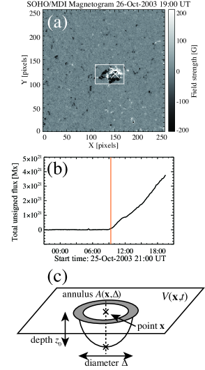
Doppler observations of NOAA AR 10488 (Figure 1(a)) from Michelson Doppler Imager (MDI; Scherrer et al., 1995) on board the Solar and Heliospheric Observatory (SOHO) are used in this work. Time-evolution of the total unsigned magnetic flux in this AR is plotted as Figure 1(b). The tracked Doppler dataset (AR data) has a cadence of 1 min with a duration of 24 hr from 19:30 UT, 2003 October 25 (about 14 hr before the flux appearance) and a size of pixels with a pixel size of 0.12 degree in the heliographical coordinates. For comparison we also use the Doppler data at the same disk location but 17 days later when there was no active region (QS data). Here it should be noted that each dataset has some temporal gaps (periods of no observation) in the whole 24 hr data 222 AR data: 19:53–20:01 UT on October 25th and 05:11–05:19 UT on 26th. QS data: 02:57–03:05 UT and 13:12–13:26 UT on November 12th. . According to Hartlep et al. (2011), the gaps may cause significant variations in the power. Therefore, in the 24 hr data, we discuss the power evolution only between 06:00–12:00 UT, during which there is no temporal gap, to avoid the effect of the gap.
First we eliminate the signal below and above from Fourier-transformed data both in AR and QS, using a box-car filter in the frequency domain with a hyperbolic-tangent roll-off. To eliminate the contribution of the f-mode, we also apply a high-pass filter with a Gaussian roll-off. Then we consider two types of Fourier filters, one of which is applied to the both datasets. The first type of filters is a series of phase-speed filters constructed based on the parameters used in Zhao et al. (2012). The second type is ridge filters which extract the power of p1, p2, and p3-modes. The ridge filters are constructed by approximating the location of each ridge and have a box-car shape in the frequency domain with hyperbolic-tangent roll-offs. The properties of the filters are listed in Table 1.
To determine the depth to which each filter is most sensitive, we examined how the filtered power is distributed over the phase speed , by constructing a histogram indicating the power, for each phase-speed bin, summed over the corresponding – bins. We identify the mode of this distribution as the effective phase speed, and then find the target depth as the asymptotic inner turning point corresponding to this phase speed, using the model S of Christensen-Dalsgaard et al. (1996). The target depth and its error, which is determined from the width of the histogram, are shown in Table 1. Here, and are the angular frequency and horizontal wavenumber of a sound wave, respectively.
Finally, we produce the acoustic power maps from the filtered Doppler velocity data. In order to increase the S/N ratio, the acoustic power at the point at the time , , is given as the squared velocity averaged over an annulus of a diameter of one travel distance centered at , :
| (1) |
where is the filtered velocity and is the area of a pixel element. The schematic illustration of the power calculation is shown as Figure 1(c). If the acoustic wave is affected by the power-reducing agent at the bottom of the ray path, the observed acoustic power in the annulus will be reduced. For a higher S/N, the thickness of the annulus is made twice as broad as shown in Table 1. The obtained maps show the temporal and two-dimensional evolution of acoustic powers at six different depths.
3 Results
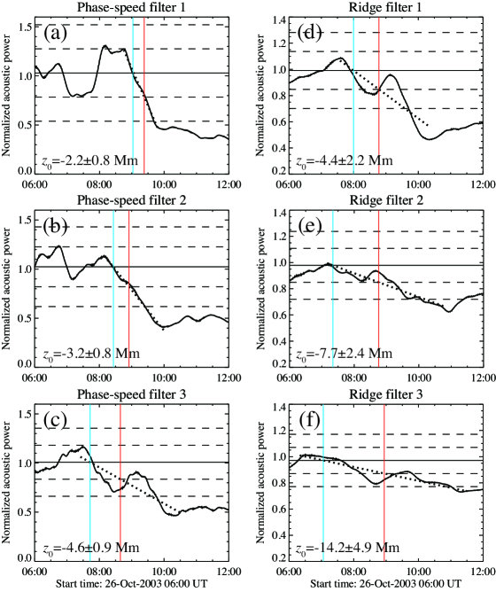
Figure 2 shows the temporal evolutions of acoustic power that correspond to six different depth ranges by phase-speed filters (a–c) and ridge filters (d–f). In each panel, the plotted curve is the acoustic power from AR data at the location of flux emergence , normalized by the power at the same location but from QS data: . We apply 60-min running average (30-min from the target time) to smooth measurements, both in AR and QS, to reduce rapid fluctuations that may not correspond to the subsurface magnetic field. The horizontal lines are the mean, , and levels calculated from the quiet regions surrounding the emerging AR. Here, one can see that the acoustic powers, which are more or less unity before 08:00 UT, fall below level around 10:00 UT. Considering that the flux of AR 10488 appears at around 09:20 UT by the method introduced in Toriumi et al. (2012), the power reduction seems to be highly related to the magnetic field of this emerging AR. The amount of the reduction is basically larger for shallower filters. The shallowest filter, in Panel (a), reveals the reduction up to 65%.
To see the timing of the power reduction in Figure 2, we fit a linear trend to the curve and measure the “mean-crossing” (reduction start) and “-crossing” (significant reduction) times. The start of the fitting interval is the last peak greater than the mean level that comes before the reduction slope and the end is the point where the slope becomes flattened below the level. It is easily seen that the mean-crossing times are before 09:00 UT, namely, before the flux appearance at the photosphere, and that the mean-crossing time becomes earlier with depth. Here, the deepest filter, in Panel (f), shows the earliest reduction, which is more than 2 hr before the flux appearance.
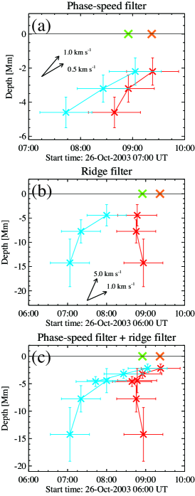
Figure 3 shows the depth-time evolution of the “mean-crossing” and “-crossing” of each filter for (a) phase-speed filter, (b) ridge filter, and (c) both. Here, the mean-crossings in Panels (a) and (b) show upward trends from deeper to shallower with time. In this figure, we also plot the occurrence of the horizontal divergent flow (HDF), which is the manifestation of the plasma escaping from the rising magnetic field, and the flux emergence at the surface, using the method developed by Toriumi et al. (2012). Therefore, this figure indicates that the rising patterns come before the flux emergence, or even before the HDF appearance at the visible surface. The mean-crossing of the ridge filters ( to Mm) show a fast rising pattern first at the rate of several , then at , while that of the phase-speed filters ( to Mm) show the slower rate of . In Figure 3(c), one can clearly see the decelerating trend of the mean-crossing times, which will be discussed in detail in the next section. We confirmed that even if we expand the fitting intervals in Figure 2 by 40 minutes, at the cost of increased degree of misfit, the mean- and -crossing times shift by less than 15 minutes (within the horizontal error bars in Figure 3c) and thus the rising speed does not change much.
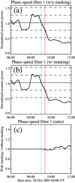
It is known that the acoustic power is suppressed in the surface magnetic fields. Vertical fields may cause mode conversion of the acoustic waves into down-going slow mode waves, leading to power reduction. Other reduction mechanisms include energy conversion into thermal energy, enhanced leakage to atmosphere due to changes in cut-off frequency, emissivity reduction, local suppression, etc. (see Chou et al., 2009). Numerous observations and theoretical works have widely been carried out in this field (e.g., Braun et al. 1987 for sunspots, Jain et al. 2009 for plage regions, and Chitta et al. 2012 for small magnetic elements in quiet region). In order to examine the effect of the surface field, at least the direct and local effects, we compare the acoustic power calculated with and without masking the strong surface field in the averaging annulus. Figure 4(a) shows the temporal evolution of the normalized acoustic power for the shallowest filter (here we call “without masking”), which is the same as Figure 2(a). To reduce the effect of the field, we also calculated the power by excluding the pixels with field strength greater than G from the averaging annulus (“with masking”), which is shown as Figure 4(b). Here, the fitted (dotted) line is found to be just the same as that in Panel (a), and thus the mean-crossing and -crossing times do not change. Panel (c) shows the ratio of the power (b) with masking over (a) without masking. Here, the ratio is deviated from unity in the later time, which indicates that in fact we see the effect of the surface field. However, when the flux first appears at 09:20 UT, the difference is less than 5%, which increases afterward but remains less than 10%. It is because the fraction of magnetized pixels to the total number of pixels in the annulus is small (of the order of a few percent). As for the other five deeper filters, the difference is much smaller and the mean- and -crossing times do not change at all. Therefore, we can conclude that, although the emergence starts at 09:20 UT and the temporal power-smoothing has a 30-min window from the target time, the effect of the surface field on the power reduction at around and before 08:50 UT is fairly negligible. Note that this masking method does not remove the surface field effect perfectly, since weaker pixels (field strength ) may also be affected by the surrounding fields and unresolved kG strength flux tubes may exist in such pixels. Thus, wave absorption or mode conversion by surface fields (maybe associated with the rising flux) may play a role in the observed acoustic power reduction, particularly after the emergence of the flux. To measure to which extent the surface field affects our measurements, we need to repeat our analysis on many more regions, e.g., regions with similar flux distributions but without emerging ARs, or with other ARs.
4 Discussion and Conclusions
As is evident in Figure 3, before the emerging flux appears at the visible surface, the onset of the acoustic power reduction starts from the deeper layers, and the speed of the rising trend gradually changes from several to less than in the shallower convection zone (), suggesting the deceleration of the power-reducing agent. If we assume that this is actually a magnetic field, Figure 3 means that the magnetic flux shows the rising motion, first at the rate of in the – Mm depth range, then at the rate of in – Mm, finally at in – Mm. This gradual deceleration of the emerging magnetic flux is well in line with the theoretical “two-step emergence” model by Toriumi & Yokoyama (2010). In this model, the emerging flux in the uppermost convection zone is decelerated because of the photospheric layer ahead of the flux, which then triggers the magnetic buoyancy instability to penetrate the photosphere, and eventually restart rising into the solar atmosphere, leaving an HDF just before the flux appearance at the visible surface. The deceleration may be more effective in the shallower layer above Mm, since, at around Mm, the radius of the rising flux tube exceeds the local pressure scale height (Fan, 2009), which encourages the mass accumulation and the resultant deceleration. By considering this model, we can speculate that the deceleration in the shallower layer and the flux appearance at the surface shown in Figure 3 are the manifestation of the two-step emergence model.
In Ilonidis et al. (2011), the average emergence speed of the magnetic flux in AR 10488 from Mm to the surface is estimated to be , while, in Ilonidis (2012), the speed from to Mm is estimated to be . Also, from the thin-flux-tube simulation, the rising speed is about at Mm (Fan, 2009). In the present study, the rising speed between and (namely, of the order of ), measured from the five filters in the upper , are consistent with previous studies. In addition, we find that the flux went through in the upper within hours, which is also in agreement with previous helioseismic studies (Kosovichev, 2009).
One important factor we should take into account is the difference of the sensitivity to the power reduction between the two types of the filters (phase-speed filters and ridge filters), or even among the filters of the same group but for different depths. Here we expect that the measurements of the power-reduction due to rising magnetic fields will be less sensitive when the fields are at larger depths, since (1) large depths are probed by acoustic waves with large horizontal wavelengths and, for large wavelengths, the absorption may be less effective, and (2) the conversion of acoustic waves into slow MHD waves, one of the main power-reduction mechanisms (Cally et al., 2003), is probably less effective at large depths, where the gas pressure dominates over the magnetic pressure. It was also shown that, in the case of sunspot fields, the absorption coefficient drops to almost zero at depths of about – (Ilonidis & Zhao, 2011), which is the target depth of the deepest filter. Here the rising speed is simply calculated from the difference of target depths of two filters over the detection time difference. If the deepest filter is less sensitive, the detection time by this filter might be later than the actual time and thus the rising speed might be overestimated at .
These uncertainties make it difficult to directly compare the power reduction events in Figure 3. Therefore, a clear identification of the power-reducing agent requires much work, which we shall leave for future research. Nevertheless, we find a rising motion which is related to the flux emergence, prior to the flux appearance at the photosphere.
In this Letter we apply a set of phase-speed filters and ridge filters to the SOHO/MDI Dopplergrams of the emerging AR 10488 to see the acoustic power reduction at different depths. In summary, our results show the following:
-
1.
All of the investigated acoustic powers show reductions, up to more than 2 hr before the flux appearance at the photosphere.
-
2.
In both filter groups, the start times of the power reduction show a rising trend and a gradual deceleration. The trend speed is first in the 15–10 Mm depth range, then in 10–5 Mm, finally in 5–2 Mm.
-
3.
If we assume that the power reduction is caused by a magnetic field corresponding to AR 10488, the detected deceleration is well in accordance with the two-step emergence model of the emerging magnetic field. This study observationally supports the theoretical two-step model.
-
4.
The estimated emerging speeds of about are highly consistent with other observations and numerical simulations. The speed at larger depths, however, may be overestimated with this method. We should examine and improve the present analysis method and investigate how sensitive each filter is to the target region, and what the detected object actually is.
Although this work shows a promising result, here we just analyzed one particular set of AR and QS. Therefore, we need to repeat our measurements on many more regions.
References
- Braun et al. (1987) Braun, D. C., Duvall, Jr., T. L., & Labonte, B. J. 1987, ApJ, 319, L27
- Cally et al. (2003) Cally, P. S., Crouch, A. D., & Braun, D. C. 2003, MNRAS, 346, 381
- Chitta et al. (2012) Chitta, L. P., Jain, R., Kariyappa, R., & Jefferies, S. M. 2012, ApJ, 744, 98
- Chou et al. (2009) Chou, D.-Y., Liang, Z.-C., Yang, M.-H., & Sun, M.-T. 2009, Sol. Phys., 255, 39
- Christensen-Dalsgaard et al. (1996) Christensen-Dalsgaard, J., Dappen, W., Ajukov, S. V., et al. 1996, Science, 272, 1286
- Duvall (2003) Duvall, Jr., T. L. 2003, ESA Special Publication, 517, 259
- Fan (2009) Fan, Y. 2009, Living Reviews in Solar Physics, 6, 4
- Hartlep et al. (2011) Hartlep, T., Kosovichev, A. G., Zhao, J., & Mansour, N. N. 2011, Sol. Phys., 268, 321
- Ilonidis et al. (2011) Ilonidis, S., Zhao, J., & Kosovichev, A. 2011, Science, 333, 993
- Ilonidis & Zhao (2011) Ilonidis, S. & Zhao, J. 2011, Sol. Phys., 268, 377
- Ilonidis (2012) Ilonidis, S. 2012, PhD thesis, Stanford University
- Jain et al. (2009) Jain, R., Hindman, B. W., Braun, D. C., & Birch, A. C. 2009, ApJ, 695, 325
- Kosovichev (2009) Kosovichev, A. G. 2009, Space Sci. Rev., 144, 175
- Moreno-Insertis & Emonet (1996) Moreno-Insertis, F. & Emonet, T. 1996, ApJ, 472, L53
- Parker (1955) Parker, E. N. 1955, ApJ, 121, 491
- Scherrer et al. (1995) Scherrer, P. H., Bogart, R. S., Bush, R. I., et al. 1995, Sol. Phys., 162, 129
- Toriumi & Yokoyama (2010) Toriumi, S. & Yokoyama, T. 2010, ApJ, 714, 505
- Toriumi & Yokoyama (2011) Toriumi, S. & Yokoyama, T. 2011, ApJ, 735, 126
- Toriumi & Yokoyama (2012) Toriumi, S. & Yokoyama, T. 2012, A&A, 539, A22
- Toriumi et al. (2012) Toriumi, S., Hayashi, K., & Yokoyama, T. 2012, ApJ, 751, 154
- Zhao et al. (2012) Zhao, J., Couvidat, S., Bogart, R. S., et al. 2012, Sol. Phys., 275, 375
| Filter # | Target depth | Phase speed | Annulus range |
|---|---|---|---|
| [Mm] | [] | [Mm] | |
| Phase-speed filteraa The phase speed and annulus range are cited from Zhao et al. (2012), while the target depth is calculated from the model S of Christensen-Dalsgaard et al. (1996).: | |||
| 1 | 6.6–9.5 | ||
| 2 | 9.5–12.4 | ||
| 3 | 13.1–16.0 | ||
| Ridge filterbbAfter the filtering, the effective phase speed is evaluated, then the depth and annulus range are calculated from the model S.: | |||
| 1 | 7.1–15.5 | ||
| 2 | 13.7–24.3 | ||
| 3 | 22.0–46.2 |