Novel variational model for inpainting in the wavelet domain

Abstract

Wavelet domain inpainting refers to the process of recovering the missing coefficients during the image compression or transmission stage. Recently, an efficient algorithm framework which is called Bregmanized operator splitting (BOS) was proposed for solving the classical variational model of wavelet inpainting. However, it is still time-consuming to some extent due to the inner iteration. In this paper, a novel variational model is established to formulate this reconstruction problem from the view of image decomposition. Then an efficient iterative algorithm based on the split-Bregman method is adopted to calculate an optimal solution, and it is also proved to be convergent. Compared with the BOS algorithm the proposed algorithm avoids the inner iteration and hence is more simple. Numerical experiments demonstrate that the proposed method is very efficient and outperforms the current state-of-the-art methods, especially in the computational time.

1 Introduction

In the image science, the term “inpainting” means recovering the missing data in images. It is an important task in various image restoration problems including scratch removal, impulse noise removal, zooming and so on. These mentioned applications are all related to the inpainting in the image domain. However, in the real storage and transmission of the digital images, the discrete wavelet transform is a very popular method for the sparse coding. For example, in the JPEG2000 image compression standard, the images are formatted in the wavelet domain. Then part of the wavelet coefficients has to be discarded or may be corrupted during the compression and transmission process, which may lead to serious degradation of the visual quality of the images especially when the loss appears in the coarsest low-low subband. Therefore, in order to improve the visual quality, the missing or corrupted coefficients should be recovered from the known information. This generates another important inpainting process in the wavelet domain, which is the core problem discussed here.

Inpainting in the image domain, which uses the values of the available pixels to fill the missing pixels, has been widely investigated in the last two decades. Bertalmio et al. [1] introduced the partial differential equations (PDEs) to smoothly propagate the information from the neighboring pixels into the areas contain the unknown pixels. Later, Chan and Shen proposed the total variation (TV) inpainting model [2], which derives from the well-known Rudin-Osher-Fatemi (ROF) model and aims at minimizing the TV norm in the process of filling the missing pixels. Further, higher order methods such as the curvature-driven diffusion (CDD) [3] and Euler’s elastica based variational model [4] were also applied to the inpainting problem in order to overcome the block effects caused by the TV model. These edge-preserved methods are unable to recover the texture regions efficiently. Therefore, the exemplar-based texture synthesis techniques [5] [6] were developed for recovering the textured images. The similar idea was also applied to image denoising and then non-local mean filter was proposed by Buades et al. [7]. Based on this method, non-local total variation [8][9][10] was further investigated and applied in various image restoration problem including the inpainting task. These non-local techniques are more suitable for recovering the texture and fine details of images than the previous local methods.

The wavelet domain inpainting is a completely different problem since missing or damaged wavelet coefficients could cause degradation widely spread in the pixel domain. Specifically, the loss of different wavelet subbands leads to different degradation types on the visual quality of images. For example, the loss of the high frequencies in the coarsest subbands creates Gibbs artifacts or other blur effects, and the loss in the coarsest low-low subband creates regular or irregular big black squares in the image domain [11]. Due to the damaged regions caused by the wavelet loss cannot be well defined in the pixel domains, the block-based inpainting methods [12] [13] such as image domain inpainting or interpolation algorithms, which were widely used for the restoration of the JPEG compressed images based on block DCT transforms, aren’t well suitable for the inpainting in the wavelet domain.

These novel features and challenges prompt the need of developing new models and methods of image inpainting in the wavelet domain. An important guiding principle is to control the regularization in the image domain with the wavelet domain constraints, so that the reconstruction images could retain the important geometrical features such as the sharp edges. Inspired by this idea, the hybrid variational models were introduced as an alternative class of approaches. Durand et al. [14] used the TV minimization technique to recover the missing/corrupted wavelet coefficients. Chan et al. [15] proposed both the constrained/unconstrained variational models combining the TV regularization term and the wavelet coefficients fitting. The authors also investigated the properties of the models such as the existence and uniqueness. Besides, other edge-preserved regularization term with different properties were also applied to this problem [16] [17]. However, the classical total variation and other local-gradient based methods are not suitable for images with fine structures, details and textures. Then similarly to the inpainting in the image domain, Zhang et al. [11] extended the TV wavelet inpainting model to the corresponding non-local (NL) form, and proposed an efficient iterative algorithm called Bregmanized operator splitting (BOS) to solve the TV/NL-TV wavelet inpainting models.

In fact, these models discussed above are all established as special cases of variational image restoration problem. However, the characteristic of wavelet domain inpainting itself inspires us to consider the problem from another view of image decomposition— the original image is divided into two components: one is just the known image constructed by the coefficients in the known domain, and the other is the rest image decided by the missing coefficients. Inspired by this viewpoint, we establish a novel variational model to recover the missing coefficients based on TV/NL-TV prior for the original image, and propose a fast iterative algorithm based on the split-Bregman method.

The rest of the paper is organized as follows: several classical wavelet inpainting models and corresponding fast algorithms are introduced in section 2. In section 3 we propose a new variational model for the inpainting problem in the view of image decomposition, and investigate the corresponding fast algorithm. In section 4 the existence of solutions of the corresponding minimization problem are investigated and the convergence of the proposed iterative algorithm is proved. In section 5 we focus on the implementation of the proposed algorithm, and compare our model with previous works. The conclusion about the proposed algorithm is given in section 5.

2 Related works

Let $f\in L^{2}(\Omega)$ be the original image defined on the bounded region $\Omega$, the standard orthogonal wavelet expansion of $f$ is denoted by

$$f(\alpha,x)=\sum_{j,k}\alpha_{j,k}\psi_{j,k}(x),~{}~{}j\in\mathbb{Z},k\in\mathbb{Z}^{2}$$

where $x\in\Omega$, and $\alpha_{j,k}$ denotes wavelet coefficients of $f$ at level $j$ and location $k$ under the wavelet basis $\{\psi_{j,k}\}$. Assume that the wavelet coefficients in the index region $I$ are known, that is,

$$\beta_{j,k}=\begin{cases}\alpha_{j,k},\quad\ \ &(j,k)\in I,\\ 0,\quad\ \ &else.\end{cases}$$

The aim of wavelet domain inpainting is to reconstruct the wavelet coefficients of $f$ using the given coefficients $\beta_{j,k}$. In [15] Chan et al. investigated the TV model for the inpainting problems. Precisely, the following constrained and unconstrained TV inpainting model (corresponding to the noise-free and noise case) are considered:

$$\min_{\alpha_{j,k}}\textrm{TV}(f(\alpha,x))~{}~{}s.t.~{}~{}\alpha_{j,k}=\beta_{j,k},$$ (2.1)

and

$$\min_{\alpha_{j,k}}\textrm{TV}(f(\alpha,x))+\sum_{j,k}\lambda_{j,k}(\alpha_{j,k}-\beta_{j,k})^{2}$$ (2.2)

where $\lambda_{j,k}$ are regularization parameters, and the total variation term is defined by

$$\textrm{TV}(f)=\textrm{sup}\left\{\int_{\Omega}f~{}\textrm{div}\vec{\phi}~{}dx:\vec{\phi}\in(C_{0}^{\infty}(\Omega))^{2},\|\vec{\phi}\|_{\infty}\leq 1\right\}.$$

Assume that $f\in W^{1,1}(\Omega)$, then we further have $\textrm{TV}(f)=\int_{\Omega}|\nabla f|dx$.

Let $W:L^{2}(\Omega)\rightarrow L^{2}(\Omega)$ denote the orthogonal wavelet transform, and $P_{I}$ denote the projection operator onto the known index set $I$, i.e.

$$P_{I}(\alpha)_{j,k}=\begin{cases}\alpha_{j,k},\quad\ \ &(j,k)\in I,\\ 0,\quad\ \ &else.\end{cases}$$

Using a general convex regularization function $J(\cdot)$ instead of the TV term, then the above minimization problems can be rewritten as

$$\min_{f}J(f)~{}~{}s.t.~{}~{}P_{I}Wf=\beta,$$ (2.3)

and

$$\min_{f}J(f)+\lambda\|P_{I}Wf-\beta\|^{2}_{2}.$$ (2.4)

Let $A=P_{I}W$, then both formulations (2.3) and (2.4) are special cases of the inverse restoration problem. Therefore, a number of methods for solving the general inverse problem such as the subgradient projection [18], the Newton-like method [19], the split-Bregman/Augmented Lagrangian method [20] [21] [22], and the primal-dual method [23] [24] [25] can also be applied to solve the unconstrained problem (2.4). On the other hand, the constrained form is a different problem. In [11], Zhang et al. used an efficient algorithm called BOS to calculate a optimal solution of the constrained problem (2.3). The BOS was introduced in [26], which use the Bregman iteration [28] to solve the equality constrained problem (2.3), i.e.

$$\left\{\begin{array}[]{lll}f^{k+1}=\textrm{arg}\min_{f}\{\mu J(f)+\frac{1}{2}\|Af-\beta^{k}\|^{2}\},&{}&{}\\ \beta^{k+1}=\beta^{k}+(\beta-Af^{k+1}),&{}&{}{}\end{array}\right.$$ (2.5)

and the sub-minimization problem in (2.5) is solved by the proximal Forward-Backward Splitting algorithm (PFBS) [27]: let $f^{k+1,0}=f^{k}$, for $i>0$

$$f^{k+1,i}=arg\min_{f}J(f)+\frac{1}{2\delta\mu}\left\|f-(f^{k+1,i}-\delta A^{T}(Af^{k+1,i}-\beta^{k}))\right\|^{2}.$$ (2.6)

In the above formulas, $\mu$ and $\delta$ are positive parameters. In order to recover images which contain rich textures or fine structures, Zhang et al. also extended the TV inpainting model to the non-local TV form, where the NL-TV regularization term can be expressed as follows:

$$\int_{\Omega}|\nabla_{w}f|(x)dx=\int_{\Omega}\sqrt{\int_{\Omega}(f(y)-f(x))^{2}w(x,y)dy}dx$$ (2.7)

where $x,y\in\Omega$ and $w(x,y)$ denotes the weight function related to pixels $x$ and $y$. For more details refer to [8] [11].

3 The proposed inpainting model

In this section, we consider the inpainting problem from another view of image decomposition. For convenience the following discussion is based on the discrete setting, that is, let $\Omega=[1,\sqrt{n}]\times[1,\sqrt{n}]$, $f\in\mathbb{R}^{n}$ be the original image and $W\in\mathbb{R}^{n\times n}$ be the orthogonal wavelet transform matrix. Assume $\tilde{W}=W^{-1}$ is the inverse wavelet transform, $\alpha_{I}$ and $\alpha_{I^{c}}$ are vectors formed by the wavelet coefficients of the original image $f$ corresponding to the known index set $I$ and its complementary set. Then we have

$$f=\tilde{W}\alpha=\tilde{W}\alpha_{I}+\tilde{W}\alpha_{I^{c}}=f_{0}+\tilde{W}\alpha_{I^{c}}.$$

To observe the above relationship, the original image is decomposed into two components—the observed image $f_{0}$ which is decided by the known coefficients, and the unknown part which represents the missing coefficients. This inspires us to estimate the missing information directly based on certain priors about the original image.

To this end, utilizing the regularization prior such as the TV/NL-TV norm for the image $f$ and the above relationship, we could establish the following minimization problem:

$$\min_{f,\alpha_{m}\in C}J(f)~{}~{}s.t.~{}~{}f=f_{0}+\tilde{W}\alpha_{m}$$ (3.1)

where $J$ is the regularization function such as the TV/NL-TV norm, and the set

$$C=\{\gamma:P_{I}(\gamma)=\textbf{0}\}.$$

In fact, we observe that the component $f_{0}$ in the proposed model can be substituted by any observed image $f^{*}$ such that $P_{I}Wf^{*}=\alpha_{I}$.

Let $\iota_{C}$ be the indicator function of set $C$, i.e.

$$\iota_{C}(\gamma)=\begin{cases}0,\quad\ \ &\gamma\in C,\\ +\infty,\quad\ \ &\gamma\not\in C.\end{cases}$$

Then the problem (3.1) can be rewritten as

$$\min_{f,\alpha_{m}}J(f)+\iota_{C}(\alpha_{m})~{}~{}s.t.~{}~{}f=f_{0}+\tilde{W}\alpha_{m}.$$ (3.2)

The split-Bregman method can be used to solve the proposed model. Considering a general constrained problem of the form

$$\min_{u}\hat{J}(u)~{}~{}s.t.~{}~{}u\in\mathbb{R}^{m},~{}~{}Mu=d$$ (3.3)

where $\hat{J}$ is a closed, proper, convex function, $d\in\mathbb{R}^{n}$, and $M\in\mathbb{R}^{n\times m}$ is a bounded linear operator. The Bregman iteration [28] for (3.3) can be reformulated as

$$\left\{\begin{array}[]{lll}u^{k+1}=\textrm{arg}\min_{u}\left\{\hat{J}(u)+\frac{\lambda}{2}\|b^{k}+Mu-d\|^{2}\right\}&{}&{}{}\\ b^{k+1}=b^{k}+(Mu^{k+1}-d)&{}&{}\end{array}\right.$$ (3.4)

By identifying $(f,\alpha_{m}),J(f)+\iota_{C}(\alpha_{m}),\tilde{W}\alpha_{m}-f$, and $-f_{0}$ as $u,\hat{J}(u),Mu$ and $d$, the Bregman iteration for problem (3.2) is

$$\left\{\begin{array}[]{lll}(f^{k+1},\alpha_{m}^{k+1})=\textrm{arg}\min_{f,\alpha_{m}}\left\{J(f)+\iota_{C}(\alpha_{m})+\frac{\lambda}{2}\|b^{k}+f_{0}+\tilde{W}\alpha_{m}-f\|^{2}\right\},&{}&{}{}\\ b^{k+1}=b^{k}+(f_{0}+\tilde{W}\alpha_{m}^{k+1}-f^{k+1}).&{}&{}\end{array}\right.$$ (3.5)

In the above iteration, the sub-minimization problem can be solved by the alternative minimization approach, that is,

$$\left\{\begin{array}[]{lll}\alpha_{m}^{k+1}=\textrm{arg}\min_{\alpha_{m}}\left\{\iota_{C}(\alpha_{m})+\frac{\lambda}{2}\|b^{k}+f_{0}+\tilde{W}\alpha_{m}-f^{k}\|^{2}\right\},&{}&{}{}\\ f^{k+1}=\textrm{arg}\min_{f}\left\{J(f)+\frac{\lambda}{2}\|b^{k}+f_{0}+\tilde{W}\alpha_{m}^{k+1}-f\|^{2}\right\}.&{}&{}{}\\ \end{array}\right.$$ (3.6)

The first sub-minimization problem in (3.6) has the closed solution as follows

$$\alpha_{m}^{k+1}=P_{C}\left(W(f^{k}-f_{0}-b^{k})\right)$$

where $P_{C}$ denotes the projection to the set $C$, which is just to set the coefficients on the index set $I$ to be zeros and keep others unchanged. Moreover, for the general case of non-orthogonal wavelet transform such as redundant transform and tight frames, $\tilde{W}$ is not orthogonal, but still has full rank. Let $\hat{W}$ be the matrix which is constructed by columns of $\tilde{W}$ corresponding to the index in set $I^{c}$, then the non-zero elements of $\alpha_{m}^{k+1}$ can be obtained by $\hat{W}^{{\dagger}}(f^{k}-f_{0}-b^{k})$, where $\hat{W}^{\dagger}$ denotes the general inverse of $\hat{W}$.

The second sub-minimization problem of the formula (3.6) has the same form as the formula (2.6), which is just the iterative step of the inner iteration of the BOS algorithm. In this paper we choose the regularization function $J$ to be TV/NL-TV norm. Thus this sub-problem corresponds to the TV or NL-TV denoising model , and it can be solved by the primal-dual or split-Bregman methods efficiently. For more details refer to [20][25]. Introducing the proximity operator [27] defined by

$$\textrm{prox}_{J}(g)={\textrm{arg}\min}\left\{\frac{1}{2}\|g-f\|^{2}_{2}+J(f)\right\},$$

the solution of the second sub-minimization problem can be expressed as $f^{k+1}=\textrm{prox}_{\frac{1}{\lambda}J}(b^{k}+f_{0}+\tilde{W}\alpha_{m}^{k+1})$.

During the implementation of Bregman iteration (3.5), it could guarantee the convergence enough to update $f^{k+1}$ and $\alpha_{m}^{k+1}$ once by the approach (3.6). This leads to the split-Bregman method for problem (3.1), which is summarized as Algorithm 1 below. Note that the true solution of the proximity operator $\textrm{prox}_{\frac{1}{\lambda}J}$ cannot be obtained in practice. However, the convergence property of the un-exact split Bregman iteration still comes into existence while the proximity operator is solved exactly enough, which will be verified in the next section.

Algorithm 1 wavelet inpainting algorithm based on the split-Bregman method

0:  observed image $f_{0}$; index set $I$ on which the wavelet coefficient information is available; wavelet transform matrix $W$; penalty parameter $\lambda$; step size $\delta$.Output: estimated image $f$. Initialization: $k=0;b^{0}=0;f^{0}=0;$Iteration:    Step1: $\alpha_{m}^{k+1}=P_{C}\left(W(f^{k}-f_{0}-b^{k})\right)$;    Step2: $f^{k+1}=\textrm{prox}_{\frac{1}{\lambda}J}(b^{k}+f_{0}+\tilde{W}\alpha_{m}^{k+1})$;    Step3: $b^{k+1}=b^{k}+(f_{0}+\tilde{W}\alpha_{m}^{k+1}-f^{k+1})$ until some stopping criterion is satisfied. Use the output of $f_{0}+\tilde{W}\alpha_{m}^{k}$ of the above loop as the final estimation of $f$.

Compared with the BOS algorithm in (2.5)-(2.6), our algorithm avoids the inner iteration for solving the sub-minimization problem in (2.5), which requires the implementation of the discrete wavelet and inverse wavelet transforms for several times, as shown in the formula (2.6). Therefore, our method could reduce the computation time efficiently. Besides, the step 3 in Algorithm 1 can be rewritten as

$$b^{k+1}=(b^{k}+f_{0}+\tilde{W}\alpha_{m}^{k+1})-f^{k+1}.$$

Due to $b^{k}+f_{0}+\tilde{W}\alpha_{m}^{k+1}$ and $f^{k+1}$ are both obtained in the step 2, only one implementation of wavelet and inverse wavelet transforms is needed in each iteration.

4 The analysis of the proposed model

In the following, we choose the regularization function $J$ to be TV/NL-TV norm, and then address the existence of the solution of problem (3.1). To this end, we require that the inverse wavelet transform matrix $\tilde{W}$ satisfies the following condition: there exists a positive constant $\varepsilon$ such that for any $\alpha\in C$,

$$\|L\circ\tilde{W}\alpha\|_{2}\geq\varepsilon\|\alpha\|_{2},$$ (4.1)

where $L$ denotes the local or non-local gradient operator $\nabla$ or $\nabla_{w}$. While $J$ is chosen to be the NL-TV norm, we further assume that the weight $w(x,y)$ is fixed in this section, otherwise the function $J$ is non-convex. Then based on some basic results of convex analysis we can show the existence of the minimizer. It is stated as follows.

Theorem 4.1

Assume that the inverse wavelet transform matrix $\tilde{W}$ satisfies the inequality (4.1), the minimization problem (3.1) has at least one solution.

Proof 1

The problem (3.1) can be rewritten as

$$\min_{\alpha\in C}J(f_{0}+\tilde{W}\alpha).$$

It is simple to verify that the set $C$ is nonempty closed convex. To prove the existence of the minimizer to problem (3.1), it suffices to show that $J(f_{0}+\tilde{W}\alpha)$ is convex and coercive with respect to $\alpha$. Due to the function $J$ is the TV or NL-TV regularization term, it satisfies the triangle inequality. Thus the convexity of $J(f_{0}+\tilde{W}\alpha)$ is a direct result.

Next, we show that $J(f_{0}+\tilde{W}\alpha)$ is coercive. Since $\tilde{W}$ satisfies the inequality (4.1),

$$J(f_{0}+\tilde{W}\alpha)\geq J(\tilde{W}\alpha)-J(-f_{0})\geq\|L\circ\tilde{W}\alpha\|_{2}-J(-f_{0})\geq\varepsilon\|\alpha\|_{2}-J(f_{0}).$$

Clearly, if $\|\alpha\|_{1}\rightarrow\infty$, then $J(f_{0}+\tilde{W}\alpha)\rightarrow\infty$, which completes the proof.

The equivalence between the split Bregman algorithm and the alternating direction method of multipliers (ADMM) has been widely researched in some previous works [29][30]. Then based on the convergence result of the ADMM proposed by Eckstein and Bertsekas [30], the convergence of the proposed algorithm can be addressed for the ideal case where the subproblem in step 2 of Algorithm 1 is solved exactly. To this end, we review the general theorem by Eckstein and Bertsekas in which convergence of a generalized version of ADMM is discussed.

Theorem 4.2

(Eckstein-Bertsekas) Considering an unconstrained problem of the form

$$\min_{z\in\mathbb{R}^{n},u\in\mathbb{R}^{m}}F(z)+G(u),~{}~{}s.t.~{}~{}Bz+Du=p,$$ (4.2)

where $B\in\mathbb{R}^{l\times n},D\in\mathbb{R}^{l\times m}$, and $p\in\mathbb{R}^{l}$. Assume that $F$ and $G$ are closed proper convex functions, $D$ has full column rank and $F(z)+\|Bz\|_{2}^{2}$ is strictly convex. Suppose $\{\varepsilon_{k}\}$ and $\{\eta_{k}\}$ be two sequences such that $\varepsilon_{k}\geq 0$, $\eta_{k}\geq 0$, $\sum_{k=0}^{\infty}\varepsilon_{k}<\infty$ and $\sum_{k=0}^{\infty}\eta_{k}<\infty$. Consider three sequences $\{u^{k}\},\{z^{k}\},\{b^{k}\}$ satisfy

$$\left\|u^{k+1}-\textrm{arg}\min_{u}\left\{G(u)+\frac{\lambda}{2}\|b^{k}+Bz^{k}+Du-p\|^{2}\right\}\right\|\leq\varepsilon_{k},$$ (4.3)

$$\left\|z^{k+1}-\textrm{arg}\min_{z}\left\{F(z)+\frac{\lambda}{2}\|b^{k}+Bz+Du^{k+1}-p\|^{2}\right\}\right\|\leq\eta_{k},$$ (4.4)

$$b^{k+1}=b^{k}+Bz^{k+1}+Du^{k+1}-p,$$ (4.5)

where $\lambda$ is a positive parameter. If the set of the solutions of (4.2) is nonempty, the sequence $\{u^{k}\},\{z^{k}\}$ converges to one solution of (4.2).

Next we discuss the convergence of the proposed algorithm. In order to guarantee the convergence, we require that the second sub-minimization problem in (3.6) is solved exactly enough. Precisely, let

$$\epsilon_{k}=f^{k}-\textrm{prox}_{\frac{1}{\lambda}J}(b^{k-1}+f_{0}+\tilde{W}\alpha_{m}^{k}),$$ (4.6)

the error should satisfy

$$\Sigma_{k\geq 1}\|\epsilon_{k}\|_{2}<\infty.$$ (4.7)

Then the convergence of Algorithm 1 is stated as follows.

Theorem 4.3

Let the assumptions of Theorem 4.1 hold true, and the obtained $\{f^{k}\}$ in step 2 of Algorithm 1 satisfies the formulas (4.6) and (4.7). Then the sequence $\{f^{k}\}$ generated by Algorithm 1 converges to one solution of (3.1).

Proof 2

By identifying $f,\alpha_{m},-I,\tilde{W},-f_{0},J(f),\iota_{C}(\alpha_{m})$ in problem (3.2) as $z,u,B,D,p,F(z),G(u)$ in problem (4.2), it suffices to show that:

(i) $J(f),\iota_{C}(\alpha_{m})$ are closed proper convex functions with respect to $f$ and $\alpha_{m}$ respectively;

(ii)the matrix $\tilde{W}$ has full column rank;

(iii)$J(f)+\|f\|^{2}_{2}$ is strictly convex.

$J(f)$ is the TV/NL-TV regularization term. Thus the closed proper convexity is a direct consequence of the definition. The conditions in (i) come into existence. The operator $J$ is also a bounded operator, thus according to the assumption in (4.1) we conclude that $\tilde{W}^{T}\tilde{W}>0$ and hence $\tilde{W}$ has full column rank. Therefore, the conditions in (ii) exist. Since the function $\|f\|^{2}_{2}$ is strictly convex, the conditions in (iii) also exist.

Then according to the Eckstein-Bertsekas theorem, the sequence $\{f^{k}\}$ generated by Algorithm 1 converges to one solution of (3.1).

5 Numerical examples

In this section, we evaluate the performance of the proposed algorithm and compare it with the BOS algorithm for wavelet domain inpainting [11]. Four images (size of $256\times 256$): Barbara, Lena, Cameraman and GoldHill are used for our tests, and all the experiments are performed under Windows XP and MATLAB 2010 running on a Lenovo laptop with a Dual Intel Pentium CPU 1.8G and 1 GB of memory.

In all simulated examples presented in the section, we use Daubechies 7-9 wavelets with symmetric extensions at the boundaries [31], which is adopted in standard JPEG2000 for lossy compression. 4-scale wavelet decomposition is used for the images in the test. As is usually done, the standard Peak Signal to Noise (PSNR) is used to quantify the performance of wavelet coefficient filling:

$$PSNR(f_{ori},f)=10\lg\left\{\frac{1}{\|f_{ori}-f\|_{2}}\right\}$$ (5.1)

where $f_{ori}$ and $f$ denote the original image and the restored image respectively.

For the weight function $w(x,y)$ in the NL-TV regularization (2.7), we use the same setting as that adopted in [11], i.e., the patch size and the searching window for the semi-local weight are fixed as 5 and 15 and the 10 best neighbors and 4 nearest neighbors are chosen for the weight computation of each pixel. For both the BOS algorithm in [11] and the proposed algorithm, the TV denoising (see the formula (2.6) or step 2 of the proposed algorithm) is solved by the PDHG method, and the non-local TV version is solved by the split-Bregman method, for more details refer to [11].

In all the following experiments, we choose $\mu=0.05$ for TV, $\mu=0.01$ for nonlocal TV, and $\delta=1$ for the BOS algorithm shown in (2.5)-(2.6). The maximum inner iterations of the PFBS are set as 10. For the proposed algorithm, the parameter $\lambda$ for TV is set to be 10, and $[30,50]$ is a proper interval for the value of $\lambda$ in the non-local TV case. Moreover, we use the error limitation as the stopping criterion. Precisely, $\|P_{I}Wf-\beta\|_{2}<10^{-5}$ and $\|f-f_{0}-\tilde{W}\alpha_{m}\|_{2}<10^{-5}$ are used for both algorithms.

In [11], the author use the image generated only by the known coefficients as the initial image in the case of some wavelet coefficients loss but keeping all low-low frequencies. However, the received image is in very poor quality while part of the LL frequencies are lost. Therefore, an interpolated image (obtained by applying the nearest neighbor interpolation on the LL subband) is used as the initial guess for the BOS algorithm in this case. For our method, we choose the known component $f_{0}$ by the same strategy.

The Barbara image is used in the first experiment. $\lambda=30$ is adopted in the proposed algorithm with the non-local regularization. We consider the case of the lowest HL subband loss for the test image. Due to the information missing happens in high frequency subands, we observe that Gibbs artificial or other blur effects appears in the received image shown in Figure 1(b). The restored images by the TV and NL-TV methods are shown in the second and third rows of Figure 1. Next, the case of random loss of wavelet coefficients is considered. Figure 2(a) shows the received image with $60\%$ randomly chosen coefficients. We observe that many black squares appear in the image due to the LL frequencies loss. The restored images by using both approaches are shown in the second and third rows of Figure 2. From these results we observe that the proposed method produces the better PSNRs with much less computational time than the BOS algorithm. In order to make the results more clearly, we also describe how the PSNR is improved by the proposed method and the BOS algorithm as the time increases. The plots in Figure 3 show the evolution of PSNR against CPU time, which verify the efficiency of the proposed method.

(a) Original image

(b) Received image, PSNR=29.13dB

(c) TV-BOS, PSNR=31.92dB, iter=15, CPU time=128.12s

(d) TV-Algorithm 1, PSNR=32.03dB, iter=15, CPU time=13.39s

(e) NLTV-BOS, PSNR=34.31dB, iter=15, CPU time=778.38s

(f) NLTV-Algorithm 1, PSNR=34.41dB, iter=25, CPU time=224.73s

Figure 1: Whole HL subband ($32\times 32$) loss. (a)Original image, (b)received image, (c)the result by BOS algorithm with TV, (d)the result by Algorithm 1 with TV, (e)the result by BOS algorithm with NL-TV, (f)the result by Algorithm 1 with NL-TV.

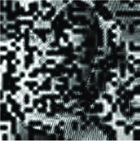
(a) Received image

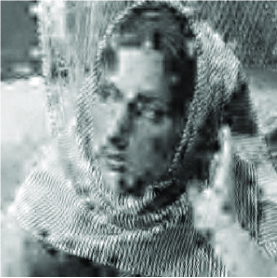
(b) Interpolated image, PSNR=19.65dB

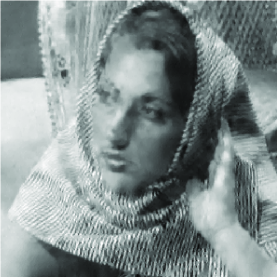
(c) TV-BOS, PSNR=22.09dB, iter=15, CPU time=131.31s

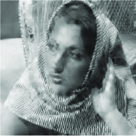
(d) TV-Algorithm 1, PSNR=22.15dB, iter=15, CPU time=13.05s

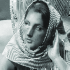
(e) NLTV-BOS, PSNR=24.84dB, iter=25, CPU time=1336.7s

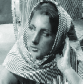
(f) NLTV-Algorithm 1, PSNR=24.85dB, iter=25, CPU time=223.61s

Figure 2: Random loss: $60\%$ random chosen frequencies. (a)Received image, (b)restored image by applying the nearest neighbor interpolation on the LL subband, (c)the result by BOS algorithm with TV, (d)the result by Algorithm 1 with TV, (e)the result by BOS algorithm with NL-TV, (f)the result by Algorithm 1 with NL-TV.

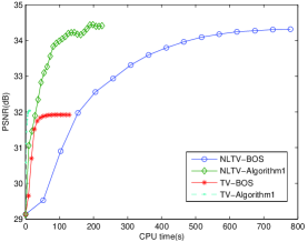
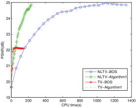
Figure 3: Evolution of PSNR against CPU time with the Barbara image. (a)The evolution curves of different methods for the received image in Figure 1, (b)the evolution curves of different methods for the received image in Figure 2.

In the second experiment the standard image Lena is used for our test. We set $\lambda=50$ for the non-local TV case in the the proposed algorithm. First we consider the case that the lowest LH subband is lost. The received image with certain edge blurring effects is shown in Figure 4 (b), and the restored images obtained by the BOS algorithm and our method are presented in the second and third rows of Figure 4. Second, the case of random coefficients loss in the high frequencies is considered. Figure 5(a) shows the $50\%$ randomly chosen high-frequency coefficients and all low-low frequencies on the top left, and 5(b) is the corresponding image. Both algorithms with TV/NL-TV regularization are implemented and the results are shown as Figure 5(c)-(f). The plots in Figure 6 show the evolution of PSNR against CPU time. Once again we observe that the proposed method can achieve the same PSNRs much faster than the BOS algorithm.

(a) Original image

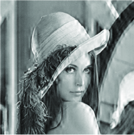
(b) Received image, PSNR=24.88dB

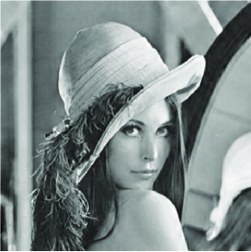
(c) TV-BOS, PSNR=31.34dB, iter=15, CPU time=129.08s

(d) TV-Algorithm 1, PSNR=31.32dB, iter=20, CPU time=19.37s

(e) NLTV-BOS, PSNR=33.36dB, iter=15, CPU time=835.16s

(f) NLTV-Algorithm 1, PSNR=33.39dB, iter=25, CPU time=222.42s

Figure 4: Whole LH subband ($32\times 32$) loss. (a)Original image, (b)received image, (c)the result by BOS algorithm with TV, (d)the result by Algorithm 1 with TV, (e)the result by BOS algorithm with NL-TV, (f)the result by Algorithm 1 with NL-TV.

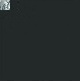
(a) Received wavelet coefficients

(b) Received image, PSNR=22.65dB

(c) TV-BOS, PSNR=26.10dB, iter=15, CPU time=130.33s

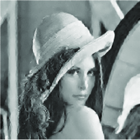
(d) TV-Algorithm 1, PSNR=26.08dB, iter=15, CPU time=13.61s

(e) NLTV-BOS, PSNR=26.83dB, iter=15, CPU time=824.55s

(f) NLTV-Algorithm 1, PSNR=26.82dB, iter=25, CPU time=233.81s

Figure 5: Random loss: $50\%$ random chosen frequencies. (a)Received image, (b)restored image by applying the nearest neighbor interpolation on the LL subband, (c)the result by BOS algorithm with TV, (d)the result by Algorithm 1 with TV, (e)the result by BOS algorithm with NL-TV, (f)the result by Algorithm 1 with NL-TV.

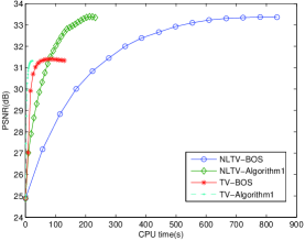
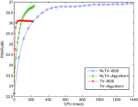
Figure 6: Evolution of PSNR against CPU time with the Lena image. (a)The evolution curves of different methods for the received image in Figure 4, (b)the evolution curves of different methods for the received image in Figure 5.

Next, the images Cameraman and GoldHill are used to test both algorithms with the TV regularization term. The four cases of wavelet coefficients missing: the whole LH and HL loss, $50\%$ random loss keeping all low-low subband frequencies, $30\%$ random loss are considered and the corresponding PSNR values and CPU time are shown in Table 1, where ’(H)’ denotes only high frequencies are randomly lost. The maximum outer iterations are set as 15 for the first three cases, and set as 25 for the last case. It is observed that our method is more efficient than the BOS algorithm in the CPU time though the PSNR values are more or less the same. Figure 7-8 shows the restored results of both images Cameraman and GoldHill with $30\%$ of their wavelet coefficients are lost randomly. We observe that the proposed algorithm requires fewer computational time than the BOS method to achieve the similar recovery effect.

Table 1: PSNR and CPU time for different methods

Image	missing case	BOS algorithm		Our method
		PSNR(dB)	Time(s)	PSNR(dB)	Time(s)
	HL loss	35.57	127.67	35.54	13.89
Cameraman	LH loss	35.98	127.61	36.19	14.30
	50$\%$ loss (H)	24.88	126.23	24.84	14.12
	30$\%$ loss	27.76	212.27	27.55	22.33
	HL loss	32.13	124.06	32.44	14.79
GoldHill	LH loss	31.87	125.55	32.22	14.18
	50$\%$ loss (H)	24.95	127.14	24.98	13.39
	30$\%$ loss	26.25	208.59	26.33	22.0

(a) Received image

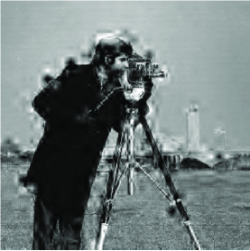
(b) Interpolated image

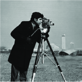
(c) TV-BOS

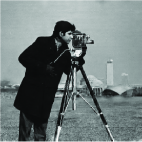
(d) TV-Algorithm 1

Figure 7: Random loss: $70\%$ random chosen frequencies. (a)Received image, (b)restored image by applying the nearest neighbor interpolation on the LL subband, (c)the result by BOS algorithm with TV, (d)the result by Algorithm 1 with TV.

(a) Received image

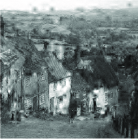
(b) Interpolated image

(c) TV-BOS

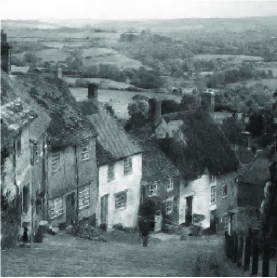
(d) TV-Algorithm 1

Figure 8: Random loss: $70\%$ random chosen frequencies. (a)Received image, (b)restored image by applying the nearest neighbor interpolation on the LL subband, (c)the result by BOS algorithm with TV, (d)the result by Algorithm 1 with TV.

Finally, we test the case when there is white Gaussian noise present in the random loss data. Similarly to the noise-free case, we use the interpolated image as the initial guess for the BOS algorithm and the known component $f_{0}$ in our method. Two images barba128 (size of $128\times 128$) and Cameraman are used for this test. Due to existence of the noise we use $f^{k}$ in Algorithm 1 as the final result, and the standard deviation $\sigma$ of the noise is used to replace the upper bound $10^{-5}$ in the stopping criterion. Figure 9 shows the results of the noisy image barba128 generated by both algorithms. It is obvious that our algorithm obtains the better results with much less implementation time. The results of Cameraman image corrupted by Gaussian noise with $\sigma=0.02$ are also shown in Figure 10 (due to the NL-TV regularization cannot produce better results for the image in this example, we don’t consider it here). It verifies the efficiency of the proposed algorithm once again.

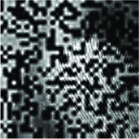
(a) Received image

(b) Interpolated image, PSNR=23.49dB

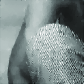
(c) TV-BOS, PSNR=23.99dB, iter=5, CPU time=27.20s

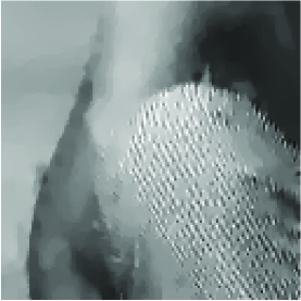
(d) TV-Algorithm 1, PSNR=24.14dB, iter=3, CPU time=0.64s

(e) NLTV-BOS, PSNR=27.94dB, iter=15, CPU time=486.95s

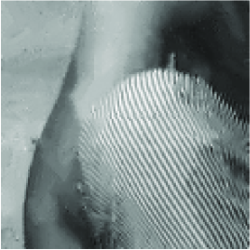
(f) NLTV-Algorithm 1, PSNR=28.35dB, iter=8, CPU time=18.16s

Figure 9: Random loss with noise: $60\%$ random chosen frequencies with noise level $\sigma=0.02$. (a)Received image, (b)restored image by applying the nearest neighbor interpolation on the LL subband, (c)the result by BOS algorithm with TV, (d)the result by Algorithm 1 with TV, (e)the result by BOS algorithm with NL-TV, (f)the result by Algorithm 1 with NL-TV

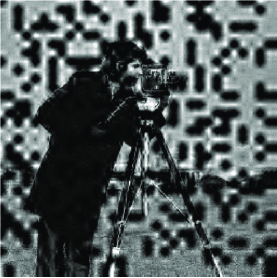
(a) Received image

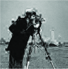
(b) Interpolated image, PSNR=20.49dB

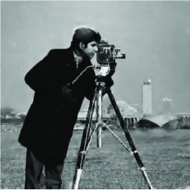
(c) TV-BOS, PSNR=25.89dB, iter=3, CPU time=28.86s

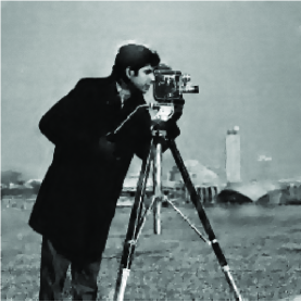
(d) TV-Algorithm 1, PSNR=25.89dB, iter=10, CPU time=9.23s

Figure 10: Random loss with noise: $70\%$ random chosen frequencies with noise level $\sigma=0.02$. (a)Received image, (b)restored image by applying the nearest neighbor interpolation on the LL subband, (c)the result by BOS algorithm with TV, (d)the result by Algorithm 1 with TV.

6 Conclusion

In this article, inspired by the idea of image decomposition we propose a novel wavelet domain inpainting model, and present a fast iterative algorithm based on the split-Bregman method to solve the corresponding minimization problem. The convergence properties of the iterative algorithms have also been researched. Numerical examples demonstrate that the proposed method is more efficient than the previous works, especially in the computational time.

References

- [1] M. Bertalmo, G. Sapiro, V. Caselles and C. Ballester, Image inpainting, In Proceedings of SIGGRAPH 2000, pp. 417-424.
- [2] T. Chan and J. Shen, Mathematical models for local nontexture inpaintings, SIAM J. Appl. Math., 62(3) (2001), 1019-1043.
- [3] T. Chan and J. Shen, Non-texture inpainting by curvature-driven diffusions, J. Vis. Commun. Image Represent., 4(12) (2001), 436-449.
- [4] T. Chan and J. Shen, Euler’s elastica and curvature-based inpainting, SIAM J. Appl. Math., 63(2) (2002), 564-592.
- [5] A. Criminisi, P. Perez and K. Toyama, Region filling and object removal by exemplar-based image inpainting, IEEE Trans. image process. 13(9) (2004), 1200-1212.
- [6] J.-F. Aujol, S. Ladjal and S. Masnou, Exemplar-based inpainting from a variational point of view, CAM Report 09-04, UCLA, 2009.
- [7] A. Buades, B. Coll and J-M. Morel, A review of image denoising algorithms, with a new one, SIAM Multiscale Model. Simul., 4(2) (2005), 490-530.
- [8] G. Gilboa and S. Osher, Nonlocal operators with applications to image processing, SIAM Multiscale Model. Simul., 7(3)(2008) 1005-1028.
- [9] D. Q. Chen and L. Z. Cheng, Alternative minimisation algorithm for non-local total variational image deblurring, IET Image Process. 4(5)(2010) 353-364.
- [10] G. Peyre, S. Bougleux and L. Cohen, Non-local regularization of inverse problems, Inverse Problems and Imaging, 5(2) (2011), 511-530.
- [11] X. Q. Zhang and T. F. Chan, Wavelet Inpainting by Nonlocal Total Variation, Inverse Problems and Imaging, 4(1)(2010), 191-210.
- [12] S. S. Hemami and R.M. Gray, Subband coded image reconstruction for lossy packed networks, IEEE Trans. Image Process., 6(4) (1997), 1466-1477.
- [13] S.D. Rane, G. Sapiro and M. Bertalmio, Structure and texture filling- in of missing image blocks in wireless transmission and compression, IEEE Trans. Image Process., 12(3) (2003), 296-303.
- [14] S. Durand and J. Froment, Reconstruction of wavelet coefficients using total variation minimization, SIAM J. Sci. Comput., 24 (2003), 1754-1767.
- [15] T. Chan, J. Shen and H. Zhou, Total variation wavelet inpainting, J. Math. Imaging Vision, 25(1) (2006), 107 C125.
- [16] A. Yau, X.C. Tai and M. Ng, L0-Norm and Total Variation for Wavelet Inpainting, In the 2nd international conference, SSVM 2009, Lecture Notes in Computer Science, pages 539-551. Springer, 2009.
- [17] H. Zhang, Q Peng and Y. Wu, Wavelet inpainting based on p-laplace operator, Acta Automatica Sinica, 33(5) (2007), 546-549.
- [18] M. Figueiredo, R. Nowak and S. Wright, Gradient projection for sparse reconstruction: application to compressed sensing and other inverse problems, IEEE Journal of Selected Topics in Signal Processing, 1(4)(2007), 586-598.
- [19] Tony F. Chan, Gene H. Golub and Pep Mulet, A nonlinear primal-dual method for total variation-based image restoration, Lecture Notes in Control and Information Sciences, Volume 219, 1996, pp 241-252.
- [20] T. Goldstein and S. Osher, The Split Bregman Method for L1 Regularized Problems, SIAM J. Imaging Sci., 2(2) (2009), 323-343.
- [21] D. Q. Chen and L. Z. Cheng, Spatially Adapted Total Variation Model to Remove Multiplicative Noise, IEEE Trans. Image Process., 21(4) (2012), 1650-1662.
- [22] C. L. Wu, J. Y. Zhang and X. C. Tai, Augmented Lagrangian method for total variation restoration with non-quadratic fidelity, Inverse Problems and Imaging, 5(1) (2011), 237-261.
- [23] Y. W. Wen, R. H. Chan and A. M. Yip, A Primal-Dual Method for Total-Variation-Based Wavelet Domain Inpainting, IEEE Trans, Image Process., 21(1) (2012), 106-114.
- [24] S. Bonettini and V. Ruggiero, On the convergence of primal-dual hybrid gradient algorithms for total variation image restoration, J. Math. Imaging Vis., (2012), in press.
- [25] M. Zhu, Fast Numerical Algorithms for Total Variation Based Image Restoration, PhD thesis, University of California, Los Angeles, 2008.
- [26] X. Q. Zhang, M. Burger, X. Bresson and S. Osher, Bregmanized Nonlocal Regularization for Deconvolution and Sparse Reconstruction, SIAM J. Imaging Sci., 3(3) (2010), 253-276.
- [27] P. L. Combettes and V. R. Wajs, Signal recovery by proximal forward- backward splitting, SIAM Multiscale Model. Simul., 4(4)(2005), 1168-1200.
- [28] S. Osher, M. Burger, D. Goldfarb, J. Xu and W. Yin, An iterative regularization method for total variation-based image restoration, SIAM Multiscale Model. and Simul, 4 (2005), 460-489.
- [29] E. Esser, Applications of Lagrangian-based alternating direction methods and connections to split Bregman, UCLA CAM Report, 09-31.
- [30] J. Eckstein and D. Bertsekas, On the Douglas-Rachford splitting method and the proximal point algorithm for maximal monotone operators, Math. Program., 55 (3) (1992), 293-318.
- [31] A. Cohen, I. Daubeches and J.C. Feauveau, Biorthogonal bases of compactly supported wavelets, Comm. Pure Appl. Math., 45(5) (1992), 485- 560.