Real Time Bid Optimization with Smooth Budget Delivery in Online Advertising

Abstract

Today, billions of display ad impressions are purchased on a daily basis through a public auction hosted by real time bidding (RTB) exchanges. A decision has to be made for advertisers to submit a bid for each selected RTB ad request in milliseconds. Restricted by the budget, the goal is to buy a set of ad impressions to reach as many targeted users as possible. A desired action (conversion), advertiser specific, includes purchasing a product, filling out a form, signing up for emails, etc. In addition, advertisers typically prefer to spend their budget smoothly over the time in order to reach a wider range of audience accessible throughout a day and have a sustainable impact. However, since the conversions occur rarely and the occurrence feedback is normally delayed, it is very challenging to achieve both budget and performance goals at the same time. In this paper, we present an online approach to the smooth budget delivery while optimizing for the conversion performance. Our algorithm tries to select high quality impressions and adjust the bid price based on the prior performance distribution in an adaptive manner by distributing the budget optimally across time. Our experimental results from real advertising campaigns demonstrate the effectiveness of our proposed approach.

1 Introduction

In recent years, the amount of ad impressions sold through real time bidding (RTB) exchanges has had a tremendous growth. RTB exchanges provide a technology for advertisers to algorithmically place a bid on any individual impression through a public auction. This functionality enables advertisers to buy inventory in a cost effective manner, and serve ads to the right person in the right context at the right time. However, in order to realize such functionality, advertisers need to intelligently evaluate each impression in real time. Demand-side platforms (DSPs) offer such a solution called real time bid optimization [13, 16] to help advertisers find the optimal bid value for each ad request in milliseconds close to a million times per second.

The process of real time bid optimization tries to maximize the campaign performance goal under the delivery constraint within the budget schedule. The performance goals typically can be specified by minimizing cost-per-click (CPC) or cost-per-action (CPA), as well as by maximizing click-through-rate (CTR) or action-rate (AR). Typically, a smooth budget delivery constraint, expressed as not buying more than a set fraction of the impressions of interest before a set time, is used to prevent the campaign from finishing the budget prematurely or avoiding a bursty spending rate. This constraint generally helps the advertisers to have sustainable influence with their ads, avoid pushing large amount of ads in peak traffic (while performance may be degraded), and explore a broader range of audience.

(a) Premature Stop

(b) Fluctuating Budget

(c) Uniform Pacing

(d) Traffic Based Pacing

(e) Performance Based Pacing

Figure 1: Illustration of different budget pacing schemes with respect to the portion of the budget spent every time interval. Integrating these plots gives the portion of the budget spend from the beginning of the day.

It is challenging to perform real time bid optimization in a RTB environment for many reasons, including the following. Firstly, the decision of placing a bid and evaluation of the bid price needs to be performed per ad request in few milliseconds. In addition, top DSPs typically receive as many as a million ad requests per second while hundreds of millions of users simultaneously explore the web around the globe. The short latency and high throughput requirements introduce extreme time sensitivity on the process. Secondly, lots of information is missing in the real time evaluation of the individual ad requests, e.g., the feedback on previous decisions has normally a long delay in practice. More specifically, the collection of click information is delayed because of the duplication removal during the logging process. On the other hand, most of the view-through actions often require up to seven days to be converted and attributed to the corresponding impressions. Finally, click and conversion events are usually very rare for non-search advertisement and therefore the variance will be large while estimating the past performance metrics.

In this paper, we present an online approach to optimize the performance metrics while satisfying the smooth delivery constraint for each campaign. Our approach first applies a control feedback loop to iteratively estimate the future spending rate in order to impose smooth delivery constraints. Then, the spending rate is used to select high quality impressions and adjust the bid price based on the prior performance distribution to maximize the performance goal.

The rest of the paper is organized as follows. In § 2, we formulate our problem and detail previous related work. In § 3, we describe our proposed approach of online bid optimization. Various practical issues encountered during bid optimization and the proposed solutions are discussed in § 4. Thorough experimental results are presented in § 5, and in § 6 we conclude by a discussion of our approach and possible future work.

2 Background and Related Work

In this section, we first formulate the problem of bid optimization as an online linear programming, and then discuss the previous related work in the literature, and explain why those proposed solutions are not suitable for our online bid optimization problem in practice.

2.1 Problem Setup

Let us consider the online bid optimization in the following settings: There are $n$ ad requests arriving sequentially ordered by an index $i$. An individual advertiser would like to make a decision represented by an indicator variable $x_{i}\in\{0,1\}$ for all $i\in\{1,\ldots,n\}$ whether to place a bid on the $i^{th}$ ad request or not. We consider a total daily budget $B\in\mathbb{R}$ as the total cost of acquiring ad inventory. Typically, advertisers would like to have smooth budget delivery constraint, expressed as not buying more than a set fraction of the impressions of interest before a set time, in place to ensure the following two situations will never occur:

• Premature Campaign Stop: Advertisers do not want their campaigns to run out of the budget prematurely in the day so as not to miss opportunities for the rest of day. Such premature budget spend is shown in Fig. 1(a) finishing the budget 6 hours early.

• Fluctuation in Spend: Advertisers would like to be able to analyze their campaigns regularly and high fluctuations in the budget makes the consistency of the results questionable. That is why a budget pacing scheme similar to what is shown in Fig. 1(b) is not suitable.

A simple, yet widely used, budget pacing scheme that meets the smooth delivery constraints is uniform pacing or even pacing shown in Fig. 1(c). In this scheme the budget is uniformly split across the day. There are two main issues with this simple scheme as follows:

• Traffic Issue: Depending on the target audience, the volume of the online traffic varies a lot throughout the day. It might be the case that during the first half of the day, we receive more relevant traffic comparing to the second half of the day; however, uniform budget pacing scheme does not allocate the budget accordingly. As a result, either we might not be able to deliver the budget by the end of the day or we might be forced to buy low quality impressions in the second half of the day. A uniform budget pacing with respect to the traffic (as opposed to with respect to the time) might resolve this issue to some extent. Such scheme is depicted in Fig. 1(d).

• Performance Issue: The quality of the online traffic changes over the course of the day for different groups of audience. Whether this quality is being measured by CPC, CPA, CTR or AR, the budget pacing algorithm should allocate most of the budget to time periods of the day with high quality. Such scheme is depicted in Fig. 1(e) and often has few picks for the periods with high quality. This potentially can cause high fluctuations that might violate smooth delivery constraints.

Balancing the traffic and performance under smooth delivery constraints is challenging. In this paper, we propose a scheme that resolves both of these issues simultaneously.

In order to enforce the smooth delivery constraints (explained further in § 1), the overall daily budget $B$ can be broken down into a sequence of time slot schedules $\{b_{1},\ldots,b_{T}\}$, where, $b_{t}\in\mathbb{R}$ represents the allocated budget to the time slot $t$, and $\sum_{t=1}^{T}\,b_{t}=B$. In the next section, we will introduce how to impose different pacing strategies to assign $b_{t}$’s in order to select higher quality impressions. Each ad request $i$ is associated with a value $v_{i}\in\mathbb{R}$ and a cost $c_{i}\in\mathbb{R}$. The value $v_{i}$ represents the true value for the advertiser if the given ad request $i$ has been seen by an audience. The cost $c_{i}$ represents the actual advertiser cost for the ad request $i$ paid to the publisher serving the corresponding impression. In summary, the bid optimization problem with smooth budget delivery constraint can be formulated as

maximize $$\;\;\sum^{n}_{i=1}v_{i}x_{i}$$

subject to $$\;\;\sum_{j\in\mathbb{I}_{t}}c_{j}x_{j}\leq b_{t}\qquad\forall t\in\{1,\ldots,T\},$$ (1)

where, $\mathbb{I}_{t}$ represents the index set of all ad requests coming in the time slot $t$. Obviously this optimization problem is an offline formulation due to the fact that the cost and value of future ad requests are not clear at the time of decision on $x_{i}$. More precisely, after the (current) incoming ad request $i$ is received, the online algorithm of bid optimization must make the decision $x_{i}$ without observing further data. For dynamic bidding campaigns, the optimization process also needs to estimate $\widehat{c}_{i}$ as the bid price at the same time. Please note that the bid price is not equivalent to the cost $c_{i}$ for the incoming ad request $i$, because the cost is determined by a second price auction in the RTB exchange. More clearly, one should bid $\widehat{c}_{i}=c_{i}+\epsilon_{i}$ to be able to win the second price auction and actually pay $c_{i}$. The value of $\epsilon_{i}$ is determined based on the auction properties and is unknown to the bidder at the bidding time.

2.2 Related Work

Eq. (2.1) is typically called online linear programming, and many practical problems, such as online bidding [8, 19], online keyword matching [21], online packing [11], and online resource allocation [7], can be formulated in the similar form. However, we do not attempt to provide a comprehensive survey of all the related methods as this has been in a number of papers [3, 6]. Instead we summarize couple of representative methods in the following.

Zhou et al. [21] modeled the budget constrained bidding optimization problem as an online knapsack problem. They proposed a simple strategy to select high quality ad requests based on an exponential function with respect to the budget period. As time goes by, the proposed algorithm will select higher and higher quality of ad requests. However, this approach has an underlying assumption of unlimited supply; i.e., there are infinite amount of ad requests in the RTB environment. This assumption is impractical especially for those campaigns with strict audience targeting constraints.

Babaioff et al. [5] formulated the problem of dynamic bidding price using multi-armed bandit framework, and then applied the strategy of upper confidence bound to explore the optimal price of online transactions. This approach does not require any information about the prior distribution. However, multi-armed bandit framework typically needs to collect feedback quickly from the environment in order to update the utility function. Unfortunately, the collection of bidding and performance information has longer delay for display advertising in RTB environment.

Agrawal et al. [3] proposed an general online linear programming algorithm to solve many practical online problems. First they applied the standard linear programming solver to compute the optimal dual solution for the data which have been seen in the system. Then, the solution for the new instance can be decided by checking if the dual solution with the new instance satisfies the constraint. The problem is that the true value $v_{i}$ and cost $c_{i}$ for the incoming ad request is unknown when it arrives to the system. If $v_{i}$ and $c_{i}$ is estimated by some statistical models or other alternative solutions, the dual solution needs to be re-computed more frequently for each campaign in order to impose budget constraints accurately. This introduces high computational cost in the real time bidding system.

3 Online Bid Optimization

In this section, we detail our method of online bid optimization. We first revisit the smooth delivery constraint and explain how we control the spending rate adaptively when each ad request comes sequentially. Afterwards, we discuss how we can iteratively apply the spending information to select ad requests and adjust their bid price to optimize the objective function.

One should recognize two different classes of campaigns: (i) Flat CPM campaigns, and, (ii) Dynamic CPM (dCPM) campaigns. The main difference between the two types is that the first one submits a flat bid price whereas the second one optimized the bid price. Both also need to decide whether to bid on an ad request. The metric for the goodness of the decision with flat CPM campaigns is typically either CTR or AR; while the metric for dCPM is typically effective CPC (eCPC) or effective CPA (eCPA). The difference between CPA and eCPA is that CPA is the goal to reach while eCPA is what is actually realized. Regardless of the type of the campaign, we try to optimize the following goal:

$$\min\;\;\;\;\text{-CTR, -AR, eCPC or eCPA}$$ (2)

$$\;\text{s.t.}\;\;\;\;|\sum_{t}^{T}\text{\bf s}(t)-B|\leq\epsilon$$

$$\qquad\;\;\left|\text{s}(t)-b_{t}\right|\leq\delta_{t}\qquad\qquad\forall t\in\{1,\ldots,T\}$$

$$\qquad\;\;eCPM\leq M$$

where the first constraint is the total daily budget constraint (where $s(t)$ is the budget spent at time slot $t$), the second constraint enforces smooth delivery according to the schedule $b_{t}$ and the third constraint requires that eCPM does not exceed the cap $M$. The last constraint makes a dCPM campaign appear like a CPM campaign in average over time, hence, the use of CPM in dCPM.

In this formulation, the optimization parameter is $b_{t}$, since the total budget $B$ and average impression cost cap $M$ are set by the advertiser. We detail our budget pacing scheme in the rest of this section and show how we improve this optimization by smart budget pacing.

3.1 Smooth Delivery of Budget

The original idea of budget pacing control is to take the daily budget as input and calculate a delivery schedule in real-time for each campaign. Based on the delivery schedule, the DSP will try to spread out the actions of acquiring impressions for each campaign throughout the day. We break down a day into $T$ time slots and in each time slot, we assign a budget to be spent by each campaign.

In the time slot $t$, the spend of acquiring inventory is considered to be proportional to the number of impressions served at that time slot; assuming the price of individual impressions for a particular campaign remains approximately constant during that time slot. In reality, the length of the time slot should be chosen such that the variance of individual impression price for each campaign is small. Our analysis shows that this assumption holds on our real data if the length of the time slot is properly chosen.

To each campaign, we assign a pacing rate for each time slot $t$. The pacing rate is defined to be the portion of incoming ad requests that this campaign would like to bid on. To see the relationship of the pacing rate with other parameters of our proposed bid optimization system, consider the following equation derived from constraints in Eq. 2.1:

$$\mbox{\bf s}(t) =\sum_{j\in\mathbb{I}_{t}}c_{j}x_{j}\propto\mbox{\bf imps}(t)$$

$$\propto\mbox{\bf reqs}(t)\frac{\mbox{\bf bids}(t)}{\mbox{\bf reqs}(t)}\frac{\mbox{\bf imps}(t)}{\mbox{\bf bids}(t)}$$ (3)

$$\propto\mbox{\bf reqs}(t)\cdot\mbox{\bf pacing\_rate}(t)\cdot\mbox{\bf win\_rate}(t)$$

Here, s$(t)$ is the dollar amount of money spent, $\text{\bf reqs}(t)$ is the number of incoming ad requests that satisfy the audience targeting constraints of the campaign, $\text{\bf bids}(t)$ is the number of ad requests that this campaign has bid on, and finally $\text{\bf imps}(t)$ is the total number of impressions of the campaign, i.e., the bids that are won in the public auction, all during the time slot $t$. With these definitions, we naturally define the ratio of bids to ad requests as pacing rate and the ratio of impressions to bids as win rate. Notice that if we assume those ad requests that satisfy the audience targeting of a certain campaign are uniformly distributed across all of the incoming ad requests, then, one can replace $\text{\bf reqs}(t)$ with some constant times the total number of incoming ad requests. That constant can be absorbed by the proportion in (3.1).

To make progress, we want to take a dynamic sequential approach in which, we get a feedback from the previous time slot spend and adjust our pacing rate for the next time slot. By working on the proportion (3.1), the pacing rate for the next time slot $t+1$ can be obtained by a simple recursive equation as follows:

$$\mbox{\bf pacing\_rate}(t\!+\!1)$$ (4)

$$=\mbox{\bf pacing\_rate}(t)\frac{\mbox{\bf s}(t\!+\!1)}{\mbox{\bf s}(t)}\frac{\mbox{\bf reqs}(t)}{\mbox{\bf reqs}(t\!+\!1)}\frac{\mbox{\bf win\_rate}(t)}{\mbox{\bf win\_rate}(t\!+\!1)}$$

$$=\mbox{\bf pacing\_rate}(t)\frac{b_{t\!+\!1}}{\mbox{\bf s}(t)}\frac{\mbox{\bf reqs}(t)}{\mbox{\bf reqs}(t\!+\!1)}\frac{\mbox{\bf win\_rate}(t)}{\mbox{\bf win\_rate}(t\!+\!1)}$$

where, $\text{\bf reqs}(t\!+\!1)$ and win_rate$(t\!+\!1)$ represent the predicted number of ad requests and the predicted winning rate for the bids in the next time slot $t+1$. One can do such predictions using historical data keeping in mind that we are only interested in the ratio of these parameters to their previous values and not necessarily their absolute values. This recursive definition introduces a simple adaptive feedback control for smooth budget pacing.

The future spend, i.e., $\text{\bf s}(t\!+\!1)$, in (4) is set to be equivalent to the ideal desired spend $b_{t\!+\!1}$ at time slot $t+1$ in order to impose the budget constraint. Different choices of $b_{t\!+\!1}$ introduces different strategies for the budget pacing. For example, one simple strategy, called uniform pacing, tries to spend the budget evenly for the given campaign throughout the day. This strategy can be easily implemented by defining future spend $b_{t\!+\!1}^{u}$ ($u$ to denote uniform) as

$$b^{u}_{t\!+\!1}\!=\!\Big{(}B\!-\!\sum_{m=1}^{t}\text{\bf s}(m)\Big{)}\frac{L(t+1)}{\sum_{m=t+1}^{T}\;L(m)}$$ (5)

where, the first factor represents the remaining budget of the day and the second factor is the ratio of the length of the time slot $t+1$ to the remaining time in the day; i.e., $L(t)$ is the length of the time slot $t$. If time slots have equal length, one can simplify (5) to get

$$b^{u}_{t\!+\!1}=\Big{(}B-\sum_{m=1}^{t}{\bf s}(m)\Big{)}\frac{1}{T-t}.$$ (6)

Uniform pacing is not necessarily the best strategy as discussed in § 2.1. We propose a strategy to spend more money on the time slots where a particular campaign has more chance to get events of interest (clicks or conversions). To do so, we look at the campaign history data and measure the performance of the campaign during each time slot. Based on this measurement, we build a discrete probability density function described by a list of click or conversion probabilities: $p_{0},\ldots,p_{T}$ assuming $T$ time-slots per day, and $\sum_{t}^{T}p_{t}=1$. Now at each time slot, we compute the ideal spending $b^{p}_{t\!+\!1}$ ($p$ to denote probabilistic) for the next time slot as

$$b^{p}_{t\!+\!1}\!=\!\Big{(}B\!-\!\sum_{m=1}^{t}\text{\bf s}(m)\Big{)}\frac{p_{t\!+\!1}\cdot L(t\!+\!1)}{\sum^{T}_{m=t\!+\!1}p_{m}\cdot L(m)}.$$ (7)

Similar to the uniform pacing case, if the time slots have equal lengths, this can be simplified to

$$b^{p}_{t\!+\!1}\!=\!\Big{(}B\!-\!\sum_{m=1}^{t}\text{\bf s}(m)\Big{)}\frac{p_{t\!+\!1}}{\sum^{T}_{m=t\!+\!1}p_{m}}.$$ (8)

In practice, it is important to notice that if $p_{j}=0$ for some $j$, then that campaign will never spend money during that time slot and hence, it will never explore the opportunities coming up during time slot $j$. To prevent this situation, one can split the budget and use a combination of the above two strategies. This way, there will be always a chance to explore all possible opportunities.

After the pacing rate is calculated, each campaign can apply this information to adaptively select certain portions of high quality impressions, as well as adjust the bid price in order to maximize the objective function. We explain those details in the next subsections.

3.2 Selection of High Quality Ad Requests - Flat CPM Campaigns

We consider two cases of flat CPM and dynamic CPM separately as the former, unlike the latter, does not need a bid price calculation. For flat CPM campaigns that always submit a fixed bid price $c^{*}$ to RTB exchanges, the goal is to simply select a set of ad requests to bid on considering the current time slot pacing rate. Since we do not know if the current incoming ad request will eventually cause a click or conversion event during the time of bid optimization, the true value of the ad request is estimated by the prediction of its CTR or AR using a statistical model. The details of the offline training process of CTR or AR prediction is described in § 3.4.

Figure 2: Illustration of our performance based budget pacing for flat CPM campaigns.

Notice that to fulfill the smooth delivery constraint, we require a minimum number of impressions given by

$$\text{\bf imps}^{*}(t)=\frac{\text{\bf s}(t)}{c^{*}}.$$

This number of impressions can be reached only if we have

$$\text{\bf bids}^{*}(t)=\frac{\text{\bf imps}^{*}(t)}{\text{\bf win\_rate}(t)}.$$

Similarly, to get these many bidding opportunities, we expect to have

$$\text{\bf reqs}^{*}(t)=\frac{\text{\bf bids}^{*}(t)}{\text{\bf pacing\_rate}(t)}.$$

Now, we are going to select these ad requests from the set of incoming ad requests whose chance of a click or a conversion is high. To do so, we construct an empirical histogram of CTR or AR distribution $q_{t}(x)$ based on the historical data for each campaign, where $q_{t}(x)$ represents the number of ad requests in time slot $t$ that are believed to have CTR or AR of $x$, e.g., see Fig. 2. Our online algorithm finds a threshold $\tau(t)$ in the time slot $t$ to filter ad requests in the region of $q_{t}(x)$ that has low CTR or AR rate such that the smooth delivery is fulfilled. Such threshold can be formulated as

$$\tau(t)=\arg\min_{x}\left|\int^{1}_{x}q_{t}(s)ds-\text{\bf reqs}^{*}(t)\right|$$ (9)

In practice, since the CTR or AR distribution $q_{t}(x)$ is not computed frequently, it introduces some oscillations for the threshold $\tau(t)$ in different time slots if $q_{t}(x)$ is not close to the current ad request distribution. Note that this mismatch is very probable since $q_{t}(x)$ is generated from historical data that might not perfectly correlate with the current reality. In order to prevent this situation, we evaluate a confidence interval of the threshold parameter $\tau(t)$. First, we incrementally update the mean $\mu_{\tau}(t)$ and variance $\sigma_{\tau}(t)$ of the threshold $\tau(t)$ using the online adaptation as follows

$$\mu_{\tau}(t)=\mu_{\tau}(t\!-\!1)+\frac{1}{t}\left(\tau(t)\!-\!\mu_{\tau}(t-1)\right)$$ (10)

$$\sigma^{2}_{\tau}(t)=\frac{t\!-\!1}{t}\sigma^{2}_{\tau}(t\!-\!1)\!+\!\frac{1}{t}\left(\tau(t)\!-\!\mu_{\tau}(t\!-\!1)\right)\left(\tau(t)\!-\!\mu_{\tau}(t)\right)$$

Second, assuming that $\tau(t)$ comes from a Gaussian distribution, we bound $\tau(t)$. The upper and lower bounds of the threshold $\tau(t)$ can be stated as $\mu_{\tau}(t)+\gamma\frac{\sigma_{\tau}(t)}{\sqrt{d}}$ and $\mu_{\tau}(t)-\gamma\frac{\sigma_{\tau}(t)}{\sqrt{d}}$, respectively, where $d$ is the number of days we looked into the history of the data to make the statistics. The critical value $\gamma=1.96$ provides $95\%$ confidence interval. The upper bound and lower bound of the CTR or AR threshold are updated in each time slot.

Putting all together, when an ad request comes to the system, its CTR or AR value is first estimated by the statistical model. If the predicted value is larger than the upper bound of the threshold, this ad request will be kept and the fixed bid price $v^{*}$ will be submitted to the RTB exchange. If the predicted value is smaller than the lower bound of the threshold, this ad request will be simply dropped without further processing. If the predicted value is in between the upper and lower bounds, the ad request will be selected at random with probability equal to pacing_rate$(t)$. This scheme, although approximate, ensures that the smooth delivery constraint is met while the opportunity exploration continues on the boundary of high and low quality ad requests.

3.3 Selection of High Quality Ad Requests - Dynamic CPM Campaigns

For dCPM campaigns, which are free to change the bid price $c_{i}$ dynamically for each incoming ad request, the goal is to win enough number of high quality impressions for less cost. We first construct bidding histogram, with $c^{*}$ being the historical average of $c_{i}$ in time slot $t$, to represent the statistics of good and bad impressions as discussed in the previous subsection. Then, starting from a base bid price, we scale the bid price up or down properly considering the current $\text{\bf pacing\_rate}(t)$ to meet the budget obligation. We explain the second step in this subsection. For simplicity and without loss of generality, we will focus on CPA campaigns.

Notice that $\text{\bf pacing\_rate}(t)$ controls the frequency of bidding; however, if the submitted bid price is not high enough, the campaign might not win the impression in the public auction. On the other hand, if the bid price is very high, then cost per action might rise (even in second price auction as the other bidders will increase their bid price too). To adjust the bid price, defining thresholds $0\leq\beta_{1}\leq\beta_{2}\leq 1$, we consider three regions for the pacing rate: (a) safe region: when $\text{\bf pacing\_rate}(t)\leq\beta_{1}$ and there is no under delivery issue due to audience targeting, (b) critical region: when $\beta_{1}\leq\text{\bf pacing\_rate}(t)\leq\beta_{2}$ and the delivery is normal, and (c) danger region: when $\beta_{2}\leq\text{\bf pacing\_rate}(t)$ and the campaign has a hard time to find and win enough impressions. We treat each of these cases separately.

Typically dCPM campaigns work towards meeting or beating a CPA goal $G$ (compared with eCPA). We use this goal value to define a base bid price $u_{i}=\text{AR}\times\text{G}$, where AR is the predicted AR for the current ad request. We discuss the estimation of the AR in the next subsection. If our campaign is in the critical region, we submit $\widehat{c}_{i}=u_{i}$ as our bid price since the campaign is doing just fine in meeting all the obligations.

For the case where our campaign is in the safe region, we start learning the best bid price from the second price auction. In particular, we consider the difference between our submitted bid price and the second price we actually pay for both good and bad impressions. If the AR estimation algorithm is a high quality classifier, one expects to see bigger differences for high quality impressions compared to low quality ones. The reason is that a good classifier typically generates high AR for high quality impressions resulting in high values of $u_{i}$ and hence a bigger difference from the second price unless all the bidders use the same or similar algorithm.

Suppose in the past we have submitted $\widehat{c}_{i}$ as our bid price and we actually paid $c_{i}$. For those impressions that led to an action, we can build the histogram of $\theta=\frac{c_{i}}{\widehat{c}_{i}}$ and find the $\theta^{*}$ to be the bottom $1$ or $2$ percentile on that histogram. We propose to submit $\widehat{c}_{i}=\theta^{*}u_{i}$ as the bid price in this case. Obviously, this scheme hurts the spending while improving the performance; however, this is not a problem because the campaign is in the safe region.

Finally, for campaigns in the danger region, we need to understand why those campaigns are in this region. There are two main reasons for underdelivery in this design: (i) The audience targeting constraints are too tight and hence, there are not enough incoming ad requests selected for a bid, and, (ii) the bid price is not high enough to win the public auction even if we bid very frequently. There is nothing we can do about the first issue, however, we can fix the second issue by boosting the bid price.

Consider a bid price cap $C$ which in reality is being set by each RTB exchange. We would like to boost the bid price with parameter $\rho^{*}\geq 1$ so that if pacing rate is greater than $\beta_{2}$, the parameter $\rho^{*}$ increases as pacing rate increases. One suggestion can be a linear increase as

$$\rho^{*}=1+\frac{C/c^{*}\,-1}{1-\beta_{2}}\left(\text{\bf pacing\_rate}(t)-\beta_{2}\right).$$ (11)

At the end we submit $\widehat{c}_{i}=\rho^{*}u_{i}$ as our bid price. Notice that $c^{*}$ as defined in the beginning of this subsection is the average historical value of $c_{i}$ and it dynamically (and slowly) changes as the market value of the impressions change.

3.4 Estimation of CTR and AR

Thus far in the paper, we based our algorithm on the top of the assumption that we have a good system to accurately estimate click through rate (CTR) and action or conversion rate (AR). In this section, we will describe how to do this estimation. Again for simplicity and without loss of generality, we will focus on AR.

This estimation plays a crucial role in bid optimization system for many reasons including the followings. Firstly, the estimated AR provides a quality assessment for each ad request helping to decide on taking action on that particular ad request. Secondly, the base bid price is set to be the estimated AR multiplied by the CPA goal, which directly affects the cost of advertising.

There are many proposals for estimating AR in the literature. Since conversions are rare events, hierarchical structure of features for each triplet combination of (user, publisher, advertiser) have been commonly used to smooth and impute the AR for the leaf nodes that do not have enough conversion events [1, 2, 13, 14, 20]. On the other hand, there are also some studies that try to cluster users based on their behaviors and interests and then estimate AR in each user cluster, e.g., see [4, 9, 16]. In addition, many standard machine learning methods, e.g., logistic regressions  [13, 17] and collaborative filtering [15], are used to combine multiple AR estimates from different levels in the hierarchy or user clusters to produce a final boosted estimate.

We use the methodology introduced in [13] and make some improvements on the top of that. In this method, we would like to find the AR for each triplet combination of (user, publisher, advertiser) by leveraging the hierarchy structure of their features. Each actual creative (the graphic ad to be shown on the page) is a leaf in the advertiser tree hierarchy. The hierarchy starts with the root and continues layer after layer by advertiser category, advertiser, insertion order, package, line item, ad and finally creative. Using the historical data, one can assign an AR to each node in this tree by aggregating total number of impressions and actions of their children as a raw estimate. Same hierarchy and raw estimations can be done for publisher and user dimensions.

After constructing all three hierarchies with initial raw estimates, we employ a smoothing algorithm similar to the one discussed in [1, 2] to adjust the raw estimates on different levels based on the similarity and closeness of (user, publisher, advertiser) triplet on the hierarchy trees. Then, for each triplet on the leaves of the trees, we run a logistic regression over the path from that leaf to the root. This scheme results in a fairly accurate estimation of AR.

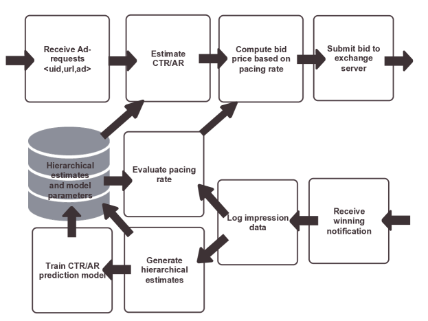
Figure 3: Illustration of ad request workflow in our proposed bid optimization framework.

4 Practical Issues

In this section, we discuss several practical issues encountered during the implementation of our proposed bid optimization method and present our current solutions.

4.1 Cold Start Problem

When a new campaign started, click or conversion events require some time to feedback to the system and therefore there is no sufficient information to perform CTR or AR estimation as well as bid optimization. This is known as cold start problem and has been well studied in the literature, e.g., see [10, 12, 18]. We follow similar ideas to apply content features such as user and publisher attributes to recommend a list of high quality websites and audience groups by inferring similarities among existing campaigns. In addition, a contextual-epsilon-greedy based strategy is performed during the online bid optimization. If the incoming ad request is inside one of those recommended publisher or audience groups, a higher bid is placed. Otherwise, the ad request will be randomly selected with a default bid price to explore unseen sites and users. As the campaign gets older and accrues more data, the activity of online exploration will be decreased and the regular prediction model will jump to play the major role of bid optimization.

4.2 Prevention of Overspending

Since budget spending is controlled by the pacing rate, if there is a huge amount of ad requests coming all of a sudden, the overall daily spend might exceed the allocated daily budget $B$. In order to overcome this problem, several monitoring processes have been implemented to frequently check the overall daily budget spend as well as the interval spend in each time slot $t$. If the overall spending exceeds the daily budget $B$, the campaign will be completely stopped. If the interval spend exceeds $b_{t}+\delta$, the bidding activity will be temporarily paused until the next time slot $t+1$.

4.3 Distributed Architecture

Fig. 3 illustrates the simplified algorithmic flow chart for each individual ad request. Please note that this workflow to submit a bid needs to happen within less than 50 milliseconds, and close to a million ad requests need to be processed in a second. Therefore, the entire bid optimization is implemented and parallelized on many distributed computing clusters cross different data centers. The offline training process utilizes R, Pig, and Hadoop to generate hierarchical CTR and AR estimates as well as train campaign-specific prediction models over a large number of campaigns. The online process streams incoming ad requests to many servers and evaluates the bid price via a real-time message bus. Our proposed algorithm works very well in this distributed environment, and detailed experimental results are presented in the next section.

Method	FC1	FC2	FC3	FC4	FC5	FC6	FC7
Our proposal	0.0159	0.0008	0.0003	0.0009	0.0005	0.0008	0.0016
Baseline	0.0041	0.0005	0.0002	0.0003	0.0002	0.0005	0.0007
Improvement (%)	286%	59%	63%	155%	132%	47%	124%

Table 1: CTR improvement for seven selected flat CPM campaigns.

5 Experimental Results

Our proposed framework of bid optimization has been implemented, tested, and deployed in Turn, a leading DSP in the Internet advertising industry. In this section, we present simulation results from our staging environment to compare different strategies of budget pacing. In addition, we also show results from real campaigns that serve large amounts of daily impressions in order to demonstrate the overall performance improvement in terms of CPC or CPA performance metrics.

5.1 Comparison of Pacing Strategies

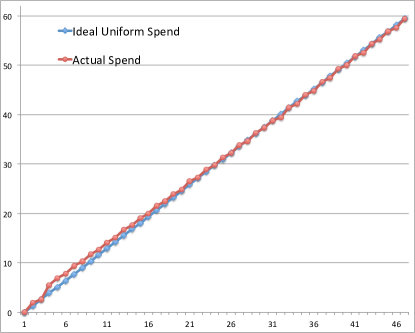
Figure 4: Simulation result of uniform budget spend. The x-axis represents the time slot, and the y-axis represents the total budget spend. The blue line depicts the ideal uniform spend, and the red line depicts the actual spend in our uniform budget pacing.

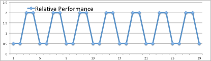
Figure 5: Relative performance across different time slot. The x-axis represents the time slot, and the y-axis represents the relative performance in terms of $\frac{1}{eCPA}$

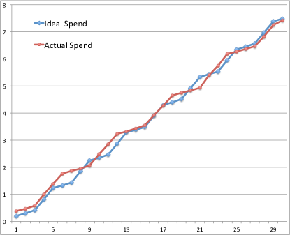
Figure 6: Simulation result of budget spend based on performance distribution. The x-axis represents the time slot, and the y-axis represents the total budget spend. The blue line depicts the ideal spend based on the performance distribution, and the red line depicts the actual spend in our performance-based budget pacing.

In this section, we would like to show the simulation results of the budget pacing in our staging environment to verify that our proposed bid optimization framework does not violate the budget constraint specified in Eq. 2.1, i.e., do not overpace or underpace. For the simulation experiment, we launch a flat CPM pseudo-campaign and assign a fixed amount of daily budget. A set of ad requests are randomly generated in each time slot. The simulation server then generates the bids based on the pacing rate and logs the winning impressions into the database.

Fig. 4 shows the ideal uniform spend and the actual spend using our uniform pacing strategy in Eq. 6. We can notice that the two lines are pretty close to each other, and the average difference across all time slots is $0.56$ dollars, which is less than $1\%$ error compared to the daily budget. Fig. 6 shows the ideal spend and the actual spend using performance based pacing strategy in Eq. 8 based on the relative performance shown in Fig. 5. We can notice that the actual spending curve indeed follows the ideal spending curve, and the average difference is $0.17$ dollars, which is about $2.3\%$ error of the daily budget.

5.2 Evaluation of Real Campaign Performance

Method	DC1a	DC2a	DC3a	DC4a	DC5a	DC6a	DC7a	DC8a	DC9a	DC10a
Our proposal	$1.32	$1.29	$7.92	$1.30	$1.98	$0.22	$2.77	$0.58	$3.23	$1.18
Baseline	$1.21	$1.12	$5.61	$0.8	$1.8	$0.21	$2.15	$0.53	$3.07	$1.16
Improvement (%)	9.4%	14.73%	41.14%	62.89%	9.95%	6.31%	28.37%	10.82%	5.41%	1.14%

Table 2: CPC improvement for ten selected dynamic CPM campaigns.

Method	DC1	DC2	DC3	DC4	DC5	DC6	DC7	DC8	DC9	DC10
Our proposal	$148.03	$3.14	$1.37	$59.32	$68.70	$186.55	$16.64	$3.76	$115.72	$200.27
Baseline	$206.39	$3.27	$1.34	$65.44	$72.95	$346.69	$22.93	$4.31	$204.62	$271.40
Improvement (%)	39.43%	4.45%	-2.23%	10.31%	6.2%	85.84%	37.78%	14.6%	76.82%	35.51%

Table 3: CPA improvement for ten selected dynamic CPM campaigns.

In this section, we evaluate the entire bid optimization framework with respect to two major classes of campaigns in our system: flat CPM campaigns and dynamic CPM campaigns. For the evaluation of flat CPM campaigns, the CTR metric is used and the higher rate represents better performance. For the evaluation dynamic CPM campaigns, CPC and CPA metrics are used based because these metrics take both total cost of impressions and the total number of clicks and conversions into account. The lower values for CPC and CPA metrics represent better performance.

We first report the performance improvement in seven active flat CPM campaigns randomly selected across different advertiser categories. Those seven campaigns were set to run based on our proposed approach and the existing baseline method. Each method was run for one week and finally two weeks of data were collected for performance comparison. Our baseline method is a simple adaptive feedback control algorithm that multiplies a constant factor to the current threshold of CTR $\tau(t)$ based on the pacing rate in the time slot $t$. The first two rows shown in Table 1 represent the CTR performance in our proposed approach and the baseline method respectively. The third row shows the percentage of improvement for each individual campaign. The average performance lift achieved by our proposed approach is $123\%$.

Next we would like to report the performance improvement for dynamic CPM campaigns. In this evaluation, we try to compare our proposed approach with the existing baseline method that only applies the pacing rate to uniformly select incoming ad requests without further adjustment of bid price. Two different sets of campaigns based on the goal type (CPC and CPA) were randomly selected across different advertiser categories. The CPC and CPA values and the percentage of performance lift for each individual campaign are shown In Table 2 and Table 3. We can observe that all twenty selected campaigns running on our proposed framework perform much better in terms of CPC and CPA metrics and the average performance lift is $19.02\%$ for CPC campaigns, and $30.87\%$ for CPA campaigns.

6 Conclusions

We have presented a general and straightforward approach to perform budget and smooth delivery constrained bid optimization for advertising campaigns in real time. Due to the simplicity of our algorithm, our current implementation can handle up to a million of ad requests per second and we think it can scale to even more. Our experimental evaluation with simulated and real campaigns shows that our proposed algorithm provides consistent improvements in standard performance metrics of CPC and CPA without underpacing or overpacing. In the future, we would like to integrate the capability of real time analytics to perform online optimization across more user, publisher, and advertiser’s attributes.

References

- [1] D. Agarwal, R. Agrawal, and R. Khanna. Estimating rates of rare events with multiple hierarchies through scalable log-linear models. ACM SIGKDD Conf. on Knowledge Discovery and Data Mining, 2010.
- [2] D. Agarwal, A. Broder, D. Chakrabarti, D. Diklic, V. Josifovski, and M. Sayyadian. Estimating rates of rare events at multiple resolutions. ACM SIGKDD Conf. on Knowledge Discovery and Data Mining, 2007.
- [3] S. Agrawal, Z. Wang, and Y. Ye. A dynamic near-optimal algorithm for online linear programming. arXiv preprint arXiv:0911.2974, 2009.
- [4] A. Ahmed, Y. Low, M. Aly, V. Josifovski, and A. J. Smola. Scalable distributed inference of dynamic user interests for behavioral targeting. ACM SIGKDD Conf. on Knowledge Discovery and Data Mining, 2011.
- [5] M. Babaioff, S. Dughmi, R. Kleinberg, and A. Slivkins. Dynamic pricing with limited supply. The 13th ACM Conference on Electronic Commerce, 2012.
- [6] M. Babaioff, N. Immorlica, D. Kempe, and R. Kleinberg. Online auctions and generalized secretary problems. ACM SIGecom Exchanges, 7(2):7, 2008.
- [7] A. Bhalgat, J. Feldman, and V. Mirrokni. Online allocation of display ads with smooth delivery. ACM SIGKDD Conf. on Knowledge Discovery and Data Mining, 2012.
- [8] C. Borgs, J. Chayes, O. Etesami, N. Immorlica, K. Jain, and M. Mahdian. Dynamics of bid optimization in online advertisement aucions. Proceeding of the 16th international conference on World Wide Web, 2007.
- [9] D. Cerrato, R. Jones, and A. Gupta. Classification of proxy labeled examples for marketing segment generation. ACM SIGKDD Conf. on Knowledge Discovery and Data Mining, 2011.
- [10] H. Cheng, R. Zwol, J. Azimi, E. Manavoglu, R. Zhang, Y. Zhou, and V. Navalpakkam. Multimedia features for click prediction of new ads in display advertising. ACM SIGKDD Conf. on Knowledge Discovery and Data Mining, 2012.
- [11] J. Feldman, M. Hezinger, N. Korula, and V. S. Mirrokni. Online stochastic packing applied to display ad allocation. ESA’10 Proceedings of the 18th annual European conference on Algorithms: Part I, 2010.
- [12] B. Kanagal, A. Ahmed, S. Pandey, V. Josifovski, L. Garcia-Pueyo, and J. Yuan. Focused matrix factorization for audience selection in display advertising. 29th IEEE International Conference on Data Engineering, 2013.
- [13] K.-C. Lee, B. Orten, A. Dasdan, and W. Li. Estimating conversion rate in display advertising from past performance data. ACM SIGKDD Conf. on Knowledge Discovery and Data Mining, 2012.
- [14] B. M. Marlin and R. S. Zemel. Collaborative prediction and ranking with non-random missing data. pages 5–12, 2009.
- [15] A. Menon, K. Chitrapura, S. Garg, D. Agarwal, and N. Kota. Response prediction using collaborative filtering with hierarchies and side-information. ACM SIGKDD Conf. on Knowledge Discovery and Data Mining, 2011.
- [16] C. Perlich and B. Dalessandro. Bid optimizing and inventory scoring in targeted online advertising. ACM SIGKDD Conf. on Knowledge Discovery and Data Mining, 2012.
- [17] M. Richardson, E. Dominowska, and R. Ragno. Predicting clicks: estimating the click-through rate for new ads. pages 521–530, 2007.
- [18] A. I. Schein, A. Popescul, L. H. Ungar, and D. Pennock. Methods and metrics for cold-start recommendations. ACM SIGIR Conf. on Information Retrieval, 2002.
- [19] W. Zhanbg, Y. Zhang, B. Gao, Y. Yu, X. Yuan, and T.-Y. Liu. Joint optimization of bid and budget allocation in sponsored search. ACM SIGKDD Conf. on Knowledge Discovery and Data Mining, 2012.
- [20] L. Zhang and D. Agarwal. Fast computation of posterior mode in multi-level hierarchical models. Neural Information Processing Systems Foundation, 2008.
- [21] Y. Zhou, D. Chakrabarty, and R. Lukose. Budget constrained bidding in keyword auctions and online knapsack problems. Proceeding of the 17th international conference on World Wide Web, 2008.