Blind Adaptive Reduced-Rank Detectors for DS-UWB Systems Based on Joint Iterative Optimization and the Constrained Constant Modulus Criterion

Abstract

A novel linear blind adaptive receiver based on joint iterative optimization (JIO) and the constrained constant modulus (CCM) design criterion is proposed for interference suppression in direct-sequence ultra-wideband (DS-UWB) systems. The proposed blind receiver consists of two parts, a transformation matrix that performs dimensionality reduction and a reduced-rank filter that produces the output. In the proposed receiver, the transformation matrix and the reduced-rank filter are updated jointly and iteratively to minimize the constant modulus (CM) cost function subject to a constraint. Adaptive implementations for the JIO receiver are developed by using the normalized stochastic gradient (NSG) and recursive least-squares (RLS) algorithms. In order to obtain a low-complexity scheme, the columns of the transformation matrix with the RLS algorithm are updated individually. Blind channel estimation algorithms for both versions (NSG and RLS) are implemented. Assuming the perfect timing, the JIO receiver only requires the spreading code of the desired user and the received data. Simulation results show that both versions of the proposed JIO receivers have excellent performance in suppressing the inter-symbol interference (ISI) and multiple access interference (MAI) with a low complexity.

Index Terms–DS-UWB systems, blind adaptive receiver, reduced-rank methods, interference suppression, CCM.

I Introduction

Ultra-wideband (UWB) technology [1]-[5], which can achieve very high data rate, is a promising short-range wireless communication technique. By spreading the information symbols with a pseudo-random (PR) code, direct sequence (DS)-UWB technique enables multiuser communications [6]. In the DS-UWB systems, a high degree of diversity is achieved at the receiver due to the large number of resolvable multipath components (MPCs) [7]. Receivers are required to efficiently suppress the severe inter-symbol interference (ISI) that is caused by the dense multipath channel and the multiple-access interference (MAI) that is caused by the lack of orthogonality between signals at the receiver in multiuser communications.

Blind adaptive linear receivers [8]-[14] are efficient schemes for interference suppression as they offer higher spectrum efficiency than the adaptive schemes that require a training stage. Low complexity blind receiver designs can be obtained by solving constrained optimization problems based on the constrained constant modulus (CCM) or constrained minimum variance (CMV) criterion [12],[15]. The blind receiver designs based on the CCM criterion have shown better performance and increased robustness against signature mismatch over the CMV approaches [12],[14]. Recently, blind full-rank stochastic gradient (SG) and RLS adaptive filters based on the constrained optimization have been proposed for multiuser detection in DS-UWB communications [15],[16]. For DS-UWB systems in which the received signal length is large due to the long channel delay spread, the interference sensitive full-rank adaptive schemes experience slow convergence rate. In the large filter scenarios, the reduced-rank algorithms can be adopted to accelerate the convergence and provide an increased robustness against interference and noise.

By projecting the received signal onto a lower-dimensional subspace and adapting a lower-order filter to process the reduced-rank signal, the reduced-rank filters can achieve faster convergence than the full-rank schemes [17]-[26]. The existing reduced-rank schemes include the eigen-decomposition methods and the Krylov subspace schemes. The eigen-decomposition methods include the principal components (PC) [17] and the cross-spectral metric (CSM) [18], which are based on the eigen-decomposition of the estimated covariance matrix of the received signal. In the PC scheme, the received signal is projected onto a subspace associated with the largest eigen-values [19] and in the CSM approach, the subspace is selected with maximum signal to interference and noise ratio (SINR) [20]. It is known that the optimal representation of the input data can be obtained by the eigen-decomposition of its covariance matrix $\mathbf{R}$ [21]. However, these methods have very high computational complexity and the robustness against interference is often poor in heavily loaded communication systems [19]. The Krylov subspace schemes include the powers of R (POR) [22], the multistage Wiener filter (MSWF) [19],[21] and the auxiliary vector filtering (AVF) [24]. All these schemes project the received signal onto the Krylov subspace [22] and achieve faster convergence speed than the full-rank schemes with a smaller filter size. However, the high computational complexity is also a problem of the Krylov subspace methods.

For the UWB systems, the reduced-rank receivers that require training sequences have recently been developed in [33]-[37]. Solutions for reduced-rank channel estimation and synchronization in single user UWB systems have been proposed in [33]. For multiuser detection in UWB communications, reduced-rank schemes have been developed in [34]-[36] that require the knowledge of the multipath channel. We proposed a low-complexity reduced-rank interference suppression scheme for DS-UWB systems in [37], which is able to suppress both of the ISI and MAI efficiently. In [38], a blind subspace multiuser detection scheme is proposed for UWB systems which requires the eigen-decomposition of the covariance matrix of the received signal. In this work, a novel CCM based joint iterative optimization (JIO) blind reduced-rank receiver is proposed. A transformation matrix and a reduced-rank filter construct the proposed receiver and they are updated jointly and iteratively to minimize the CM cost function subject to a constraint. The proposed receiver allows information exchange between the transformation matrix and the reduced-rank filter. This distinguishing feature leads to a more efficient adaptive implementation than the existing reduced-rank schemes. Note that the constraint is necessary since it enables us to avoid the undesired local minima. The adaptive NSG and RLS algorithms are developed for the JIO receiver. In the NSG version, a low-complexity leakage SG channel estimator that was proposed in [43] is adopted. Applying an approximation to the covariance matrix of the received signal, the RLS channel estimator proposed in [43] is modified for the proposed JIO-RLS with reduced complexity. Since each column of the transformation matrix can be considered as a direction vector on one dimension of the subspace, we update the transformation matrix column by column to achieve a better representation of the projection procedure in the JIO-RLS.

The main contributions of this work are summarized as follows:

• A novel linear blind JIO reduced-rank receiver based on the CCM criterion is proposed for interference suppression in DS-UWB systems.

• NSG algorithms, which are able to facilitate the setting of step sizes in multiuser scenarios, are developed for the proposed reduced-rank receivers.

• RLS algorithms are developed to jointly update the columns of the transformation matrix and the reduced-rank filter with low complexity.

• A rank adaptation algorithm is developed to achieve a better tradeoff between the convergence speed and the steady state performance.

• The convergence properties of the CM cost function with a constraint are discussed.

• Simulations are performed with the IEEE 802.15.4a channel models and severe ISI and MAI are assumed for the evaluation of the proposed scheme against existing techniques.

The rest of this paper is structured as follows. Section II presents the DS-UWB system model. The design of the JIO CCM blind receiver is detailed in Section III. The proposed NSG and RLS versions of the blind JIO receiver are described in Section IV and V, respectively. In Section VI, a complexity analysis for the proposed receiver versions is detailed and a rank adaptation algorithm is developed for the JIO receiver. Simulation results are shown in Section VII and conclusions are drawn in Section VIII.

II DS-UWB System Model

In this work, we consider the uplink of a binary phase-shift keying (BPSK) DS-UWB system with $K$ users. A random spreading code $\mathbf{s}_{k}$ is assigned to the $k$-th user with a spreading gain $N_{c}=T_{s}/T_{c}$, where $T_{s}$ and $T_{c}$ denote the symbol duration and chip duration, respectively. The transmit signal of the $k$-th user (where $k=1,2,\dots,K$) can be expressed as

$$x^{(k)}(t)=\sqrt{E_{k}}\sum_{i=-{\infty}}^{\infty}\sum_{j=0}^{N_{c}-1}p_{t}(t-iT_{s}-jT_{c})s_{k}(j)b_{k}(i),$$ (1)

where $b_{k}(i)$ $\in$ $\{\pm 1\}$ denotes the BPSK symbol for the $k$-th user at the $i$-th time instant, $s_{k}(j)$ denotes the $j$-th chip of the spreading code $\mathbf{s}_{k}$ (where $j=1,2,\dots,N_{c}$). $E_{k}$ denotes the transmission energy of the $k$-th user. $p_{t}(t)$ is the pulse waveform of width $T_{c}$. Throughout this paper, the pulse waveform $p_{t}(t)$ is modeled as the root-raised cosine (RRC) pulse with a roll-off factor of $0.5$ [39],[40]. The channel model considered is the IEEE 802.15.4a channel model for the indoor residential environment [41]. This standard channel model includes some generalizations of the Saleh-Valenzuela model and takes the frequency dependence of the path gain into account [42]. In addition, the 15.4a channel model is valid for both low-data-rate and high-data-rate UWB systems [42]. For the $k$-th users, the channel impulse response (CIR) of the standard channel model can be expressed as

$$h_{k}(t)=\sum_{u=0}^{L_{c}-1}\sum_{v=0}^{L_{r}-1}\alpha_{u,v}e^{j\phi_{u,v}}\delta(t-T_{u}-T_{u,v}),$$ (2)

where $L_{c}$ denotes the number of clusters, $L_{r}$ is the number of MPCs in one cluster. $\alpha_{u,v}$ is the fading gain of the $v$-th MPC in the $u$-th cluster, $\phi_{u,v}$ is uniformly distributed in $[0,2\pi)$. $T_{u}$ is the arrival time of the $u$-th cluster and $T_{u,v}$ denotes the arrival time of the $v$-th MPC in the $u$-th cluster. For the sake of simplicity, we express the CIR as

$$h_{k}(t)=\sum_{l=0}^{L-1}h_{k,l}\delta(t-lT_{\tau}),$$ (3)

where $h_{k,l}$ and $lT_{\tau}$ present the complex-valued fading factor and the arrival time of the $l$-th MPC ($l=uL_{c}+v$), respectively. $L=T_{DS}/T_{\tau}$ denotes the total number of MPCs where $T_{DS}$ is the channel delay spread. Assuming that the timing is acquired, the received signal can be expressed as

$$z(t)=\sum_{k=1}^{K}\sum_{l=0}^{L-1}h_{k,l}x^{(k)}(t-lT_{\tau})+n(t),$$ (4)

where $n(t)$ is the additive white Gaussian noise (AWGN) with zero mean and a variance of $\sigma_{n}^{2}$. This signal is first passed through a chip-matched filter (MF) and then sampled at the chip rate. We select a total number of $M=(T_{s}+T_{DS})/T_{c}$ observation samples for the detection of each data bit, where $T_{s}$ is the symbol duration, $T_{DS}$ is the channel delay spread and $T_{c}$ is the chip duration. Assuming the sampling starts at the zero-th time instant, then the $m$-th sample is given by

$$r_{m}=\int_{mT_{c}}^{(m+1)T_{c}}z(t)p_{r}(t)~{}dt,~{}~{}m=1,2,\dots,M$$

where $p_{r}(t)=p_{t}^{*}(-t)$ denotes the chip-matched filter, $(\cdot)^{*}$ denotes the complex conjugation. After the chip-rate sampling, the discrete-time received signal for the $i$-th data bit can be expressed as $\mathbf{r}(i)=[r_{1}(i),r_{2}(i),\dots,r_{M}(i)]^{T}$, where $(\cdot)^{T}$ is the transposition and we can further express it in a matrix form as

$$\mathbf{r}(i)=\sum_{k=1}^{K}\sqrt{E_{k}}\mathbf{P}_{r}\mathbf{H}_{k}\mathbf{P}_{t}\mathbf{s}_{k}b_{k}(i)+\mbox{\boldmath$\eta$}(i)+\mathbf{n}(i),$$ (5)

where $\mathbf{H}_{k}$ is the Toeplitz channel matrix for the $k$-th user with the first column being the CIR $\mathbf{h}_{k}=[h_{k}(0),h_{k}(1),\dots,h_{k}(L-1)]^{T}$ zero-padded to length $M_{H}=(T_{s}/T_{\tau})+L-1$. The matrix $\mathbf{P}_{r}$ represents the MF and chip-rate sampling with the size $M$-by-$M_{H}$. $\mathbf{P}_{t}$ denotes the $(T_{s}/T_{\tau})$-by-$N_{c}$ pulse shaping matrix. In order to facilitate the blind channel estimation in a later development, we rearrange the term and express the received signal as

$$\mathbf{r}(i)=\sum_{k=1}^{K}\sqrt{E_{k}}\mathbf{P}_{r}\mathbf{S}_{e,k}\mathbf{h}_{k}b_{k}(i)+\mbox{\boldmath$\eta$}(i)+\mathbf{n}(i),$$ (6)

where $\mathbf{S}_{e,k}$ is the Toeplitz matrix with the first column being the vector $\mathbf{s}_{e,k}=\mathbf{P}_{t}\mathbf{s}_{k}$ zero-padded to length $M_{H}$. The vector $\mbox{\boldmath$\eta$}(i)$ denotes the ISI from $2G$ adjacent symbols, where $G$ denotes the minimum integer that is larger than or equal to the scalar term $T_{DS}/T_{s}$. Here, we express the ISI vector in a general form that is given by

$$\begin{split}\mbox{\boldmath$\eta$}(i)&=\sum_{k=1}^{K}\sum_{g=1}^{G}\sqrt{E_{k}}\mathbf{P}_{r}\mathbf{H}_{k}^{(-g)}\mathbf{P}_{t}\mathbf{s}_{k}b_{k}(i-g)\\ &+\sum_{k=1}^{K}\sum_{g=1}^{G}\sqrt{E_{k}}\mathbf{P}_{r}\mathbf{H}_{k}^{(+g)}\mathbf{P}_{t}\mathbf{s}_{k}b_{k}(i+g),\end{split}$$ (7)

where the channel matrices for the ISI are given by

$$\mathbf{H}_{k}^{(-g)}=\begin{bmatrix}\mathbf{0}&\mathbf{H}_{k}^{(u,g)}\\ \mathbf{0}&\mathbf{0}\end{bmatrix}~{}~{};~{}~{}\mathbf{H}_{k}^{(+g)}=\begin{bmatrix}\mathbf{0}&\mathbf{0}\\ \mathbf{H}_{k}^{(l,g)}&\mathbf{0}\end{bmatrix}.$$ (8)

Note that the matrices $\mathbf{H}_{k}^{(u,g)}$ and $\mathbf{H}_{k}^{(l,g)}$ have the same size as $\mathbf{H}_{k}$, which is $M_{H}$-by-$(T_{s}/T_{\tau})$, and can be considered as the partitions of an upper triangular matrix $\mathbf{H}_{\rm up}$ and a lower triangular matrix $\mathbf{H}_{\rm low}$, respectively, where

$$\begin{split}&\mathbf{H}_{\rm up}=\begin{bmatrix}h_{k}(L-1)&\dots&h_{k}(L-\frac{T_{DS}-(g-1)T_{s}}{T_{\tau}})\\ &\ddots&\vdots\\ &&h_{k}(L-1)\end{bmatrix}~{};\\ &\mathbf{H}_{\rm low}=\begin{bmatrix}h_{k}(0)&&\\ \vdots&\ddots&\\ h_{k}(\frac{T_{DS}-(g-1)T_{s}}{T_{\tau}}-2)&\dots&h_{k}(0)\end{bmatrix}.\end{split}$$

These triangular matrices have the row-dimension of $[T_{DS}-(g-1)T_{s}]/T_{\tau}-1=L-(g-1)T_{s}/T_{\tau}-1$. Note that when the channel delay spread is large, the row-dimension of these triangular matrices could surpass the column dimension of the matrix $\mathbf{H}_{k}$, which is $T_{s}/T_{\tau}$. Hence, in case of

$$\begin{split}&L-(g-1)T_{s}/T_{\tau}-1>T_{s}/T_{\tau},\\ i.e.~{}~{}~{}&L>gT_{s}/T_{\tau}+1,\end{split}$$ (9)

the matrix $\mathbf{H}_{k}^{(u,g)}$ is the last $T_{s}/T_{\tau}$ columns of the upper triangular matrix $\mathbf{H}_{\rm up}$ and $\mathbf{H}_{k}^{(l,g)}$ is the first $T_{s}/T_{\tau}$ columns of the lower triangular matrix $\mathbf{H}_{\rm low}$. When $L<gT_{s}/T_{\tau}+1$, $\mathbf{H}_{k}^{(u,g)}=\mathbf{H}_{\rm up}$ and $\mathbf{H}_{k}^{(l,g)}=\mathbf{H}_{\rm low}$. It is interesting to review the expression of the ISI vector via its physical meaning, since the row-dimension of the matrices $\mathbf{H}_{k}^{(u,g)}$ and $\mathbf{H}_{k}^{(l,g)}$, which is $L-(g-1)T_{s}/T_{\tau}-1$, reflects the time domain overlap between the data symbol $b(i)$ and the adjacent symbols of $b(i-g)$ and $b(i+g)$.

III Proposed Blind JIO Reduced-rank Receiver Design

Figure 1: Block diagram of the proposed blind reduced-rank receiver.

In this section, we detail the design of the proposed JIO reduced-rank receiver that is able to recover the data symbol from the noisy received signal blindly. The block diagram of the proposed receiver is shown in Fig.1. In the JIO blind linear receiver, the reduced-rank received signal can be expressed as

$$\mathbf{\bar{r}}(i)=\mathbf{T}^{H}(i)\mathbf{r}(i),$$ (10)

where $\mathbf{T}(i)$ is the $M$-by-$D$ (where $D\ll M$) transformation matrix. After the projection, $\mathbf{\bar{r}}(i)$ is fed into the reduced-rank filter $\bar{\mathbf{w}}(i)$ and the output signal is given by

$$y(i)=\bar{\mathbf{w}}^{H}(i)\mathbf{\bar{r}}(i).$$ (11)

The decision of the desired data symbol is defined as

$$\hat{b}(i)={\rm sign}(\mathfrak{R}[y(i)]).$$ (12)

where ${\rm sign}(\cdot)$ is the algebraic sign function and $\mathfrak{R}(\cdot)$ represents the real part of a complex number.

The optimization problem to be solved can be expressed as

$$\left[{\mathbf{\bar{w}}}(i),\mathbf{T}(i)\right]\\ =\mathop{\mbox{arg}}\mathop{\mbox{min}}_{{\mathbf{\bar{w}}}(i),\mathbf{T}(i)}\mathbf{J}_{\rm JIO}\big{(}\bar{\mathbf{w}}(i),\mathbf{T}(i)\big{)},$$ (13)

subject to the constraint

$$\bar{\mathbf{w}}^{H}(i)\mathbf{T}^{H}(i)\mathbf{p}=v,$$ (14)

where $\mathbf{p}=\mathbf{P}_{r}\mathbf{S}_{e}\mathbf{h}$ is defined as the effective signature vector for the desired user and $v$ is a real-valued constant to ensure the convexity of the CM cost function

$$\mathbf{J}_{\rm JIO}\big{(}\bar{\mathbf{w}}(i),\mathbf{T}(i)\big{)}=\frac{1}{2}E\left[(\left|y(i)\right|^{2}-1)^{2}\right].$$ (15)

The convergence properties of the CM cost function subject to a constraint are discussed in Appendix A.

Let us now consider the problem through the Lagrangian

$$\mathcal{L}_{\rm JIO}\big{(}\bar{\mathbf{w}}(i),\mathbf{T}(i)\big{)}=\frac{1}{2}E\left[(\left|y(i)\right|^{2}-1)^{2}\right]+\mathfrak{R}[\lambda(i)(\bar{\mathbf{w}}^{H}(i)\mathbf{T}^{H}(i){\mathbf{p}}-v)],$$ (16)

where $\lambda(i)$ is a complex-valued Lagrange multiplier. In order to obtain the adaptation equation of $\mathbf{T}(i)$, we firstly assume that $\bar{\mathbf{w}}(i)$ is fixed and the gradient of the Lagrangian with respect to $\mathbf{T}(i)$ is given by

$$\nabla_{T}\mathcal{L}_{\rm JIO}=E\left[e(i)y^{*}(i)\mathbf{r}(i)\bar{\mathbf{w}}^{H}(i)\right]+\frac{\lambda_{T}(i)}{2}{\mathbf{p}}\bar{\mathbf{w}}^{H}(i),$$ (17)

where $\lambda_{T}(i)$ is the complex-valued Lagrange multiplier for updating the transformation matrix and $e(i)=|y(i)|^{2}-1$ is defined as a real-valued error signal. Recalling the relationship $y^{*}(i)=\mathbf{r}^{H}(i)\mathbf{T}(i)\bar{\mathbf{w}}(i)$ and setting (17) to a zero matrix, we obtain

$$\mathbf{T}_{\rm opt}=\mathbf{R}_{Y}^{-1}\left(\mathbf{D}_{T}-\frac{\lambda_{T}(i)}{2}\mathbf{p}\mathbf{\bar{w}}^{H}(i)\right)\mathbf{R}_{w}^{-1},$$ (18)

where $\mathbf{R}_{Y}=E[|y(i)|^{2}\mathbf{r}(i)\mathbf{r}^{H}(i)]$, $\mathbf{D}_{T}=E[y^{*}(i)\mathbf{r}(i)\mathbf{\bar{w}}^{H}(i)]$ and $\mathbf{R}_{w}=E[\mathbf{\bar{w}}(i)\mathbf{\bar{w}}^{H}(i)]$. Using the constraint $\bar{\mathbf{w}}^{H}(i)\mathbf{T}^{H}_{\rm opt}\mathbf{p}=v$, we obtain the Lagrange multiplier

$$\lambda_{T}(i)=2\left(\frac{\mathbf{\bar{w}}^{H}(i)\mathbf{R}_{w}^{-1}\mathbf{D}_{T}\mathbf{R}_{Y}^{-1}\mathbf{p}-v}{\mathbf{\bar{w}}^{H}(i)\mathbf{R}_{w}^{-1}\mathbf{\bar{w}}(i)\mathbf{p}^{H}\mathbf{R}_{Y}^{-1}\mathbf{p}}\right)^{*}.$$ (19)

Now, we assume that $\mathbf{T}(i)$ is fixed in (16) and calculate the gradient of the Lagrangian with respect to $\mathbf{\bar{w}}(i)$, which is given by

$$\nabla_{w}\mathcal{L}_{\rm JIO}=E\left[e(i)\mathbf{T}^{H}(i)\mathbf{r}(i)y^{*}(i)\right]+\frac{\lambda_{w}(i)}{2}\mathbf{T}^{H}(i){\mathbf{p}},$$ (20)

where $\lambda_{w}(i)$ is the complex-valued Lagrange multiplier for updating the reduced-rank filter. Rearranging the terms, we obtain

$$\mathbf{\bar{w}}_{\rm opt}=\mathbf{R}_{\bar{y}}^{-1}\left(\mathbf{d}_{\bar{r}}-\frac{\lambda_{w}(i)}{2}\mathbf{T}^{H}(i)\mathbf{p}\right),$$ (21)

where $\mathbf{R}_{\bar{y}}=E[|y(i)|^{2}\mathbf{\bar{r}}(i)\mathbf{\bar{r}}^{H}(i)]$ and $\mathbf{d}_{\bar{r}}=E[y^{*}(i)\mathbf{\bar{r}}(i)]$. Using the constraint $\bar{\mathbf{w}}_{\rm opt}^{H}\mathbf{T}^{H}(i)\mathbf{p}=v$, we obtain the Lagrange multiplier

$$\lambda_{w}(i)=2\left(\frac{\mathbf{d}_{\bar{r}}^{H}\mathbf{R}_{\bar{y}}^{-1}\mathbf{T}^{H}(i)\mathbf{p}-v}{\mathbf{p}^{H}\mathbf{T}(i)\mathbf{R}_{\bar{y}}^{-1}\mathbf{T}^{H}(i)\mathbf{p}}\right)^{*}.$$ (22)

With the solutions of $\mathbf{T}_{\rm opt}$ and $\mathbf{\bar{w}}_{\rm opt}$, the NSG and RLS adaptive versions of the JIO receiver will be developed in the following sections, in which the direct matrix inversions are not required and the computational complexity is reduced. Note that when adaptive algorithms are implemented to estimate $\mathbf{T}_{\rm opt}$ and $\mathbf{\bar{w}}_{\rm opt}$, $\mathbf{T}(i)$ is a function of $\mathbf{\bar{w}}(i)$ and $\mathbf{\bar{w}}(i)$ is a function of $\mathbf{T}(i)$. Thus, the optimal CCM design is not in a closed form and one possible solution for such optimization problem is to jointly and iteratively adapt these two quantities. The joint update means for the $i$-th time instant, $\mathbf{T}(i)$ is updated with the knowledge of $\mathbf{T}(i-1)$ and $\mathbf{\bar{w}}(i-1)$, then $\mathbf{\bar{w}}(i)$ is updated with $\mathbf{T}(i)$ and $\mathbf{\bar{w}}(i-1)$. Each iterative update can be considered as one repetition of the joint update.

It should also be noted that the blind JIO receiver design requires the knowledge of the effective signature vector of the desired user, or equivalently, the channel parameters. In this work, the channel coefficients are not given and must be estimated. Here, we employ the variant of the power method introduced in [43]:

$$\mathbf{\hat{h}}(i)=\left(\mathbf{I}-\mathbf{\hat{V}}(i)/tr[\mathbf{\hat{V}}(i)]\right)\mathbf{\hat{h}}(i-1),$$ (23)

where the $L$-by-$L$ matrix is defined as

$$\mathbf{\hat{V}}(i)=\mathbf{S}_{e}^{H}\mathbf{P}_{r}^{H}\mathbf{R}^{-m}(i)\mathbf{P}_{r}\mathbf{S}_{e},$$ (24)

and $\mathbf{I}$ is the identity matrix, $tr[\cdot]$ stands for trace and we make $\mathbf{\hat{h}}(i)\leftarrow\mathbf{\hat{h}}(i)/\|\mathbf{\hat{h}}(i)\|$ to normalize the channel. $\mathbf{R}(i)=\sum^{i}_{j=1}\alpha^{i-j}\mathbf{r}(j)\mathbf{r}^{H}(j)$ and $m$ is a finite power. The estimate of the matrix $\mathbf{R}^{-1}(i)$ is obtained recursively via the matrix inversion lemma [44] and is given by

$$\mathbf{\hat{R}}^{-1}(i)=\frac{1}{\alpha}\left(\mathbf{\hat{R}}^{-1}(i-1)-(\phi(i)\mbox{\boldmath{$\kappa$}}(i))\mbox{\boldmath{$\kappa$}}^{H}(i)\right),$$ (25)

where $\alpha$ is the forgetting factor, $\mbox{\boldmath{$\kappa$}}(i)=\mathbf{\hat{R}}^{-1}(i-1)\mathbf{r}(i)$ and $\phi(i)=\left(\alpha+\mathbf{r}^{H}(i)\mbox{\boldmath{$\kappa$}}(i)\right)^{-1}$. The estimation of the inversion of the covariance matrix requires $3M^{2}+2{M}+1$ multiplications and $2M^{2}$ additions. Equation (24) requires $(m+1)M^{2}L$ multiplications and $(m+1)M^{2}L-(m+1)ML$ additions, while equation (23) requires $L^{2}$ multiplications and $L^{2}+L-1$ additions (the multiplications and additions in this work are both complex-valued operations). Note that, the matrix $\mathbf{P}_{r}\mathbf{S}_{e}$ is assumed given at the receiver.

The estimate of the effective signature vector can be finally obtained as

$$\mathbf{\hat{p}}(i)=\mathbf{P}_{r}\mathbf{S}_{e}\mathbf{\hat{h}}(i),$$ (26)

where $\mathbf{\hat{h}}(i)$ is given in (23).

IV Proposed JIO-NSG Algorithms

In this section, we develop the NSG algorithm to jointly and iteratively update $\mathbf{T}(i)$ and $\bar{\mathbf{w}}(i)$. The blind channel estimator based on the leakage SG algorithm that is proposed in [43] is implemented to provide the channel coefficients.

IV-A JIO-NSG Algorithms

The optimization problem to be solved in the NSG version is given by

$$\left[{\mathbf{\bar{w}}}(i),\mathbf{T}(i)\right]\\ =\mathop{\mbox{arg}}\mathop{\mbox{min}}_{{\mathbf{\bar{w}}}(i),\mathbf{T}(i)}\mathbf{J}_{\rm JIO}\big{(}\bar{\mathbf{w}}(i),\mathbf{T}(i)\big{)},$$ (27)

subject to $\bar{\mathbf{w}}^{H}(i)\mathbf{T}^{H}(i)\hat{\mathbf{p}}(i)=v$, where $\hat{\mathbf{p}}(i)$ is the estimated signature vector obtained via blind channel estimation that will be detailed in Section IV-B and $v$ is a real-valued constant to ensure the convexity of the cost function

$$\mathbf{J}_{\rm JIO-NSG}\big{(}\bar{\mathbf{w}}(i),\mathbf{T}(i)\big{)}=\frac{1}{2}E\left[(\left|y(i)\right|^{2}-1)^{2}\right].$$ (28)

Here, we consider the problem through the Lagrangian

$$\mathcal{L}_{\rm JIO-NSG}\big{(}\bar{\mathbf{w}}(i),\mathbf{T}(i)\big{)}=\frac{1}{2}E\left[(\left|y(i)\right|^{2}-1)^{2}\right]+\mathfrak{R}[\lambda_{N}(i)(\bar{\mathbf{w}}^{H}(i)\mathbf{T}^{H}(i)\hat{\mathbf{p}}(i)-v)],$$ (29)

where $\lambda_{N}(i)$ is a complex-valued Lagrange multiplier. For each time instant, we firstly update $\mathbf{T}(i)$ while assuming that $\bar{\mathbf{w}}(i)$ is fixed. Then we adapt $\bar{\mathbf{w}}(i)$ with the updated $\mathbf{T}(i)$.

The gradient of the Lagrangian with respect to $\mathbf{T}(i)$ is given by

$$\nabla_{T}\mathcal{L}_{\rm JIO-NSG}=E\left[e(i)y^{*}(i)\mathbf{r}(i)\bar{\mathbf{w}}^{H}(i)\right]+\frac{1}{2}\lambda_{NT}(i)\hat{\mathbf{p}}(i)\bar{\mathbf{w}}^{H}(i),$$

where $\lambda_{NT}(i)$ is the complex-valued Lagrange multiplier for updating the transformation matrix and $e(i)=|y(i)|^{2}-1$ is defined as a real-valued error signal. Using the instantaneous estimator to the gradient vector, the SG update equation is given by

$$\mathbf{T}(i+1)=\mathbf{T}(i)-\mu_{T}\left(e(i)y^{*}(i)\mathbf{r}(i)+\frac{\lambda_{NT}(i)}{2}\hat{\mathbf{p}}(i)\right)\bar{\mathbf{w}}^{H}(i),$$ (30)

where $\mu_{T}$ is the step size for the SG algorithm that updates the transformation matrix. Using the constraint of $\bar{\mathbf{w}}^{H}(i)\mathbf{T}^{H}(i+1)\hat{\mathbf{p}}(i)=v$, we obtain that

$$\lambda_{NT}(i)=2\frac{\hat{\mathbf{p}}^{H}(i)\mathbf{T}(i)\bar{\mathbf{w}}(i)-\mu_{T}e(i)y^{*}(i)\|\bar{\mathbf{w}}(i)\|^{2}\hat{\mathbf{p}}^{H}(i)\mathbf{r}(i)-v}{\mu_{T}\|\bar{\mathbf{w}}(i)\|^{2}\|\hat{\mathbf{p}}(i)\|^{2}}.$$ (31)

The NSG algorithm aims at minimizing the cost function

$$\mathbf{J}_{\rm JIO-NSG}(\mu_{T})=\frac{1}{2}\left[\left|\bar{\mathbf{w}}^{H}(i)\mathbf{T}^{H}(i+1)\mathbf{r}(i)\right|^{2}-1\right]^{2}.$$ (32)

Substituting (30) and (31) into (32) and setting the gradient vector of (32) with respect to $\mu_{T}$ to zeros, we obtain the solutions

$$\mu_{T,1}=\frac{|y(i)|-1}{|y(i)|e(i)A_{T,1}},~{}\mu_{T,2}=\frac{|y(i)|+1}{|y(i)|e(i)A_{T,1}},$$

$$\mu_{T,3}=\mu_{T,4}=\frac{1}{e(i)A_{T,1}},$$

where the real-valued scale term $A_{T,1}$ is defined as

$$A_{T,1}=\|\bar{\mathbf{w}}(i)\|^{2}\left[\|\mathbf{r}(i)\|^{2}-\frac{|\mathbf{r}^{H}(i)\hat{\mathbf{p}}(i)|^{2}}{\|\hat{\mathbf{p}}(i)\|^{2}}\right].$$

By examining the second derivative of (32) with respect to $\mu_{T}$, we conclude that $\mu_{T,1}$ and $\mu_{T,2}$ are the solutions that correspond to the minima. In this work, the $\mu_{T,1}$ is used and a positive real scaling factor $\mu_{T,0}$ is implemented that will not change the direction of the tap-weight vector. Finally, the NSG update function of $\mathbf{T}(i)$ is given by

$$\mathbf{T}(i+1)=\mathbf{T}(i)-y^{*}(i)\mu_{T,0}\mathbf{A}_{T,2}-A_{T,3}\hat{\mathbf{p}}(i)\bar{\mathbf{w}}^{H}(i).$$ (33)

where

$$\mathbf{A}_{T,2}=\frac{|y(i)|-1}{|y(i)|A_{T,1}}\left(\mathbf{r}(i)\bar{\mathbf{w}}^{H}(i)-\frac{\hat{\mathbf{p}}^{H}(i)\mathbf{r}(i)}{\|\hat{\mathbf{p}}(i)\|^{2}}\hat{\mathbf{p}}(i)\bar{\mathbf{w}}^{H}(i)\right),$$

$$A_{T,3}=\big{(}\|\bar{\mathbf{w}}(i)\|^{2}\|\hat{\mathbf{p}}(i)\|^{2}\big{)}^{-1}\big{(}\hat{\mathbf{p}}^{H}(i)\mathbf{T}(i)\bar{\mathbf{w}}(i)-v\big{)}.$$

Now, let us adapt $\bar{\mathbf{w}}(i)$ while assuming $\mathbf{T}(i)$ is fixed. The gradient of the Lagrangian with respect to $\bar{\mathbf{w}}(i)$ is given by $\nabla_{w}\mathcal{L}_{\rm JIO-NSG}=E\left[e(i)y^{*}(i)\mathbf{T}^{H}(i)\mathbf{r}(i)\right]+\frac{1}{2}\lambda_{Nw}(i)\hat{\mathbf{p}}(i)\bar{\mathbf{w}}^{H}(i)$, where $\lambda_{Nw}(i)$ is the complex-valued Lagrange multiplier for updating the reduced-rank filter. By using the instantaneous estimator of the gradient vector, the SG adaptation equation is given by

$$\bar{\mathbf{w}}(i+1)=\bar{\mathbf{w}}(i)-\mu_{w}e(i)y^{*}(i)\mathbf{T}^{H}(i)\mathbf{r}(i)-\mu_{w}\frac{\lambda_{Nw}(i)}{2}\mathbf{T}^{H}(i)\hat{\mathbf{p}}(i).$$ (34)

Using the constraint $\bar{\mathbf{w}}^{H}(i+1)\mathbf{T}^{H}(i)\hat{\mathbf{p}}(i)=v$, we have

$$\lambda_{Nw}(i)=2\frac{\hat{\mathbf{p}}^{H}(i)\mathbf{T}(i)\bar{\mathbf{w}}(i)-\mu_{w}e(i)y^{*}(i)\hat{\mathbf{p}}^{H}(i)\mathbf{T}(i)\mathbf{T}^{H}(i)\mathbf{r}(i)-v}{\mu_{w}\|\mathbf{T}^{H}(i)\hat{\mathbf{p}}(i)\|^{2}}.$$ (35)

The NSG algorithm for updating the reduced-rank filter aims at minimizing the cost function

$$\mathbf{J}_{\rm JIO-NSG}(\mu_{w})=\frac{1}{2}\left[\left|\bar{\mathbf{w}}^{H}(i+1)\mathbf{T}^{H}(i)\mathbf{r}(i)\right|^{2}-1\right]^{2}.$$ (36)

Substituting (34) and (35) into (36), the solutions of $\mu_{w}$ that correspond to a null gradient vector of (36) are given by

$$\mu_{w,1}=\frac{|y(i)|-1}{|y(i)|e(i)A_{w,1}},~{}\mu_{w,2}=\frac{|y(i)|+1}{|y(i)|e(i)A_{w,1}},$$

$$\mu_{w,3}=\mu_{w,4}=\frac{1}{e(i)A_{w,1}},$$

where the scale term is given by

$$A_{w,1}=\|\mathbf{T}^{H}(i)\mathbf{r}(i)\|^{2}-\frac{|\mathbf{r}^{H}(i)\mathbf{T}(i)\mathbf{T}^{H}(i)\hat{\mathbf{p}}(i)|^{2}}{\|\mathbf{T}^{H}(i)\hat{\mathbf{p}}(i)\|^{2}}$$

By examining the second derivative of (36) with respect to $\mu_{w}$, only $\mu_{w,1}$ and $\mu_{w,2}$ correspond to the minima of the cost function (36). Finally, by applying a positive real scaling factor $\mu_{w,0}$ to control the tap-weight vector, the adaptation equation by using $\mu_{w,1}$ is given by

$$\bar{\mathbf{w}}^{H}(i+1)=\bar{\mathbf{w}}^{H}(i)-y^{*}(i)\mu_{w,0}\mathbf{A}_{w,2}-A_{w,3}\mathbf{T}^{H}(i)\hat{\mathbf{p}}(i).$$ (37)

where

$$\mathbf{A}_{w,2}=\frac{|y(i)|-1}{|y(i)|A_{w,1}}\left(\mathbf{T}^{H}(i)\mathbf{r}(i)-\frac{\hat{\mathbf{p}}^{H}(i)\mathbf{T}(i)\mathbf{T}^{H}(i)\mathbf{r}(i)}{\|\mathbf{T}^{H}(i)\hat{\mathbf{p}}(i)\|^{2}}\mathbf{T}^{H}(i)\hat{\mathbf{p}}(i)\right),$$

$$A_{w,3}=\big{(}\|\mathbf{T}^{H}(i)\hat{\mathbf{p}}(i)\|^{2}\big{)}^{-1}\big{(}\hat{\mathbf{p}}^{H}(i)\mathbf{T}(i)\bar{\mathbf{w}}(i)-v\big{)}.$$

In the proposed JIO-NSG scheme, $\mathbf{T}(i)$ and $\bar{\mathbf{w}}(i)$ are computed jointly and iteratively. Let $c$ denotes the iteration number and define $c_{max}$ as the total number of iterations for each time instant. We have $\mathbf{T}_{0}(i)=\mathbf{T}_{c_{max}}(i-1)$ and $\bar{\mathbf{w}}_{0}(i)=\bar{\mathbf{w}}_{c_{max}}(i-1)$. For the $c$-th iteration, $\mathbf{T}_{c}(i)$ is updated with $\mathbf{T}_{c-1}(i)$ and $\bar{\mathbf{w}}_{c-1}(i)$ using (33), then $\bar{\mathbf{w}}_{c}(i)$ is trained with $\mathbf{T}_{c}(i)$ and $\bar{\mathbf{w}}_{c-1}(i)$ via (37).

It is interesting to note that the complexity of the JIO-NSG scheme could be lower than the full-rank NSG algorithm because there are many entries that are frequently reused in the update equations, for example, the scalar term $\hat{\mathbf{p}}^{H}(i)\mathbf{r}(i)$, the vectors of $\mathbf{T}^{H}(i)\hat{\mathbf{p}}(i)$ and $\mathbf{T}^{H}(i)\mathbf{r}(i)$. However, the price we pay for the complexity reduction is the requirement of extra storage space at the receiver.

IV-B Blind Channel Estimator For the NSG Version

For the JIO-NSG receiver, we rearrange the equation (24) as

$$\mathbf{\hat{V}}(i)=\mathbf{S}_{e}^{H}\mathbf{P}_{r}^{H}\mathbf{\hat{W}}(i)$$ (38)

where $\mathbf{\hat{W}}(i)=\mathbf{R}^{-m}(i)\mathbf{P}_{r}\mathbf{S}_{e}$. Here, we implement the Leakage SG algorithm to estimate $\mathbf{\hat{W}}(i)$, which can be expressed as [43]

$$\mathbf{\hat{W}}_{l}(i)=\lambda_{v}\mathbf{\hat{W}}_{l}(i-1)+\mu_{v}(\mathbf{\hat{W}}_{l-1}(i)-\mathbf{r}(i)\mathbf{r}^{H}(i)\mathbf{\hat{W}}_{l}(i-1)),$$ (39)

where $l=1,\dots,m$ is defined as the iteration index, $\lambda_{v}$ is the leakage factor and $\mu_{v}$ is the step size. Using (38), we obtain the leakage SG blind channel estimator that is given by

$$\mathbf{\hat{h}}(i)=\mathbf{\hat{h}}(i-1)-\left(\mathbf{\hat{V}}(i)\mathbf{\hat{h}}(i-1)\right)/tr[\mathbf{\hat{V}}(i)],$$ (40)

Finally, the effective signature vector of the desired user is given by

$$\mathbf{\hat{p}}(i)=\mathbf{P}_{r}\mathbf{S}_{e}\mathbf{\hat{h}}(i)$$ (41)

In terms of the computational complexity, we need $4mML$ multiplications and $3mML-mL$ additions for all the recursions in (39); $L^{2}M$ multiplications and $L^{2}M-L^{2}$ additions for (38).

The JIO-NSG version is summarized in Table. I.

TABLE I: Adaptive versions of the Proposed JIO Receiver.

NSG version:

Initialization:

$\bar{\mathbf{w}}(1)=[1,1,1,\dots,1]$, $D$-by-$1$ vector,

$\mathbf{T}(1)=[\mathbf{I}_{D}~{}|~{}\mathbf{0}]^{T}$, $M$-by-$D$ matrix.

($\mathbf{I}_{D}$ represents the $D$-by-$D$ identity matrix.)

for $i=1,2,\dots$

1: Pre-adaptation:

$\bar{\mathbf{r}}(i)=\mathbf{T}^{H}(i)\mathbf{r}(i)$, $y(i)=\mathbf{\bar{w}}^{H}(i)\bar{\mathbf{r}}(i)$,

Calculate $\mathbf{\hat{V}}(i)$ and $\mathbf{\hat{h}}(i)$ using (38) and (40), respectively,

Calculate $\mathbf{\hat{p}}(i)$ using (41),

Set $\mathbf{T}_{0}(i+1)=\mathbf{T}_{c_{max}}(i)$ and $\bar{\mathbf{w}}_{0}(i+1)=\bar{\mathbf{w}}_{c_{max}}(i)$.

2: Adaptation of $\mathbf{T}(i+1)$ and $\bar{\mathbf{w}}(i+1)$:

for $c=1,2,\dots,c_{max}$

Update $\mathbf{T}_{c}(i+1)$ using (33) with $\mathbf{T}_{c-1}(i+1)$ and $\bar{\mathbf{w}}_{c-1}(i+1)$,

Update $\bar{\mathbf{w}}_{c}(i+1)$ using (37) with $\mathbf{T}_{c}(i+1)$ and $\bar{\mathbf{w}}_{c-1}(i+1)$,

end

Set $\mathbf{T}(i+1)=\mathbf{T}_{c_{max}}(i+1)$ and $\bar{\mathbf{w}}(i+1)=\bar{\mathbf{w}}_{c_{max}}(i+1)$

4: Make Decision for the $i$-th data bit:

$\hat{b}(i)={\rm sign}(\mathfrak{R}(y(i)))$

RLS version:

Initialization:

$\bar{\mathbf{w}}(1)=[1,1,1,\dots,1]$, $D$-by-$1$ vector,

$\mathbf{t}_{d}(1)=[1,0,0,\dots,0]$ ($d=1,2,\dots,D$), $D$-by-$1$ vectors,

$\mathbf{\bar{d}}(0)=[0,0,\dots,0]$, $D$-by-$1$ vector,

$\mathbf{\hat{R}}_{y}^{-1}(0)=\mathbf{I}_{M}/\delta$, $M$-by-$M$ matrix,

$\mathbf{\hat{R}}_{\rm T}^{-1}(0)=\mathbf{I}_{D}/\delta$, $D$-by-$D$ matrix,

($\mathbf{I}_{M}$ is the $M$-by-$M$ identity matrix. $\delta$ is a positive constant.)

for $i=1,2,\dots$

1: Pre-adaptation:

$\bar{\mathbf{r}}(i)=\mathbf{T}^{H}(i)\mathbf{r}(i)$, $y(i)=\mathbf{\bar{w}}^{H}(i)\bar{\mathbf{r}}(i)$,

$\mathbf{\bar{d}}(i)=\mathbf{\bar{d}}(i-1)+\alpha\mathbf{\bar{r}}(i)y^{*}(i)$,

Estimate $\mathbf{\hat{R}}_{y}^{-1}(i)$ and $\mathbf{\hat{R}}_{\rm T}^{-1}(i)$ using (46) and (52), respectively,

Calculate $\mathbf{\hat{V}}(i)$ and $\mathbf{\hat{h}}(i)$ using (55) and (54), respectively,

Calculate $\mathbf{\hat{p}}(i)$ using (56).

2: Adaptation of $\mathbf{t}_{d}(i)$:

for $d=1,2,\dotsb,D$

Calculate $\lambda_{t,d}(i)$ using (48),

Update $\mathbf{t}_{d}(i)$ using (47),

Normalize $\mathbf{t}_{d}(i)\leftarrow\mathbf{t}_{d}(i)/\parallel\mathbf{t}_{d}(i)\parallel$.

3: Adaptation of $\bar{\mathbf{w}}(i)$:

Calculate $\lambda_{Rw}(i)$ using (53),

Update $\bar{\mathbf{w}}(i)$ using (51),

4: Make Decision for the $i$-th data bit:

$\hat{b}(i)={\rm sign}(\mathfrak{R}(y(i)))$

V Proposed JIO-RLS Algorithms

In this section we detail the RLS version of the proposed JIO scheme. In the JIO scheme, the $M$-by-$D$ (where $D\ll M$) transformation matrix can be expressed as

$$\mathbf{T}(i)=[\mathbf{t}_{1}(i),\mathbf{t}_{2}(i),\dots,\mathbf{t}_{D}(i)].$$ (42)

Note that the reduced-rank received signal can be expressed as $\mathbf{\bar{r}}(i)=\mathbf{T}^{H}(i)\mathbf{r}(i)$, whose $d$-th element is $\bar{r}_{d}(i)=\mathbf{t}_{d}^{H}(i)\mathbf{r}(i)$. Since the transformation matrix projects the received signal onto a small-dimensional subspace, these vectors $\mathbf{t}_{d}(i)$ can be considered as the direction vectors on each dimension of the subspace. For each time instant, we compute these $M$-dimensional vectors $\mathbf{t}_{d}(i)$ (where $d=1,2,\dots,D$) one by one. One of the advantages of this process method in the RLS version is that the complexity of training the transformation matrix could be reduced with an approximation which will be shown soon. In addition, this method provides a better representation of the transformation matrix and leads to better performance than the approach that updates all the columns of the projection matrix together. It should be noted that, the NSG version can also be modified to update the columns of the transformation matrix one by one, but the limited improved performance in NSG version is not worth the payment of the increased complexity.

After the projection, $\mathbf{\bar{r}}(i)$ is fed into the reduced-rank filter $\bar{\mathbf{w}}(i)$ and the output signal is given by

$$y(i)=\bar{\mathbf{w}}^{H}(i)\mathbf{T}^{H}(i)\mathbf{r}(i)=\bar{\mathbf{w}}^{H}(i)\sum^{D}_{d=1}\mathbf{t}_{d}^{H}(i)\mathbf{r}(i)\mathbf{q}_{d},$$

where $\mathbf{q}_{d}$ (where $d=1,2,\dots,D$) are the vectors whose $d$-th elements are ones, while all the other elements are zeros. In this section, an adaptive blind channel estimation is employed and $\mathbf{t}_{d}(i)$ are optimized jointly and iteratively with $\bar{\mathbf{w}}(i)$ via RLS algorithms.

V-A JIO-RLS Algorithms

In the JIO-RLS scheme, we need to solve the optimization problem

$$\left[{\mathbf{\bar{w}}}(i),\mathbf{t}_{1}(i),\dots,\mathbf{t}_{D}(i)\right]=\mathop{\mbox{arg}}\mathop{\mbox{min}}_{{\mathbf{w}}(i),\mathbf{t}_{1}(i),\dots,\mathbf{t}_{D}(i)}\mathbf{J}_{JIO-RLS}\big{(}\bar{\mathbf{w}}(i),\mathbf{t}_{1}(i),\dots,\mathbf{t}_{D}(i)\big{)},$$ (43)

subject to the constraint $\bar{\mathbf{w}}^{H}(i)\sum^{D}_{d=1}\mathbf{t}_{d}^{H}(i)\hat{\mathbf{p}}(i)\mathbf{q}_{d}=v$, where $\hat{\mathbf{p}}(i)$ is the estimated signature vector obtained via blind channel estimation that will be detailed in Section V-B. $v$ is a real-valued constant to ensure the convexity of the CM cost function:

$$\mathbf{J}_{JIO-RLS}\big{(}\bar{\mathbf{w}}(i),\mathbf{t}_{1}(i),\dots,\mathbf{t}_{D}(i)\big{)}=\frac{1}{2}\sum^{i}_{j=1}\alpha^{i-j}\left(|y(j)|^{2}-1\right)^{2},$$

where $0<\alpha\leq 1$ is the forgetting factor and $y(i)$ is the output signal at the $i$-th time instant. Let us now consider the problem through the Lagrangian

$$\begin{split}&\mathcal{L}_{JIO-RLS}\big{(}\bar{\mathbf{w}}(i),\mathbf{t}_{1}(i),\dots,\mathbf{t}_{D}(i)\big{)}=\frac{1}{2}\sum^{i}_{j=1}\alpha^{i-j}\left(\left|y(j)\right|^{2}-1\right)^{2}\\ &+\mathfrak{R}\left[\lambda_{R}(i)\big{(}\bar{\mathbf{w}}^{H}(i)\sum^{D}_{d=1}\mathbf{t}_{d}^{H}(i)\mathbf{\hat{p}}(i)\mathbf{q}_{d}-v\big{)}\right],\end{split}$$ (44)

where $\lambda_{R}(i)$ is a complex-valued Lagrange multiplier. In the proposed JIO-RLS scheme, for each time instant, we firstly update the vectors $\mathbf{t}_{d}(i)$ (where $d=1,2,\dots,D$) while assuming that $\bar{\mathbf{w}}(i)$ and other column vectors are fixed. Then we adapt the reduced-rank filter with the updated transformation matrix.

For the update of the column vectors of the transformation matrix, we can express the output signal as follows

$$y(i)=\bar{\mathbf{w}}^{H}(i)\sum^{D}_{d=1}\mathbf{t}_{d}^{H}(i)\mathbf{r}(i)\mathbf{q}_{d}=\bar{w}_{d}^{*}(i)\bar{r}_{d}(i)+\bar{\mathbf{w}}^{H}(i)\mathbf{\bar{r}}_{e}(i),$$

where the $D$-dimensional vector $\mathbf{\bar{r}}_{e}(i)$ can be obtained by calculating the reduced-rank received signal $\mathbf{\bar{r}}(i)$ and setting its $d$-th element to zero. By taking the gradient term of (44) with respect to $\mathbf{t}_{d}(i)$ and setting it to a null vector, we have $\nabla_{t_{d}}\mathcal{L}_{JIO-RLS}$$=\sum^{i}_{j=1}\alpha^{i-j}e(j)\mathbf{r}(j)$$\big{(}|\bar{w}_{d}(j)|^{2}\mathbf{r}^{H}(j)\mathbf{t}_{d}(i)$$+\bar{w}_{d}^{*}(j)\mathbf{\bar{r}}_{e}^{H}(j)\bar{\mathbf{w}}(j)\big{)}$ $+\frac{1}{2}\lambda_{t,d}(i)\bar{w}_{d}^{*}(i)\mathbf{\hat{p}}(i)=0$, where $e(i)=|y(i)|^{2}-1$ and $\lambda_{t,d}(i)$ is the complex-valued Lagrange multiplier for updating the $d$-th column vector in the transformation matrix. Rearranging the terms we obtain

$$\mathbf{t}_{d}(i)=-\mathbf{R}_{\rm d}^{-1}(i)\left(\frac{\lambda_{t,d}(i)}{2}\bar{w}_{d}^{*}(i)\mathbf{\hat{p}}(i)+\mathbf{v}_{r}(i)\right),$$ (45)

where we define the $M$-dimensional vector $\mathbf{v}_{r}(i)=\sum^{i}_{j=1}\alpha^{i-j}\bar{w}_{d}^{*}(j)\mathbf{r}(j)\big{(}e(j)\mathbf{r}_{e}^{H}(j)\bar{\mathbf{w}}(j)-\bar{w}_{d}(j)\bar{r}_{d}^{*}(j)\big{)}$ and the $M$-by-$M$ matrix $\mathbf{R}_{\rm d}(i)=\sum^{i}_{j=1}\alpha^{i-j}|\bar{w}_{d}(j)|^{2}|y(j)|^{2}\mathbf{r}(j)\mathbf{r}^{H}(j)$. Note that, $\mathbf{R}_{\rm d}(i)$ is dependent on $\bar{w}_{d}(i)$, which is the $d$-th element of the reduced-rank filter. Hence, for updating each $\mathbf{t}_{d}(i)$, we need to calculate the corresponding $\mathbf{R}_{\rm d}^{-1}(i)$ and that leads to high computational complexity. In our work, we devise an approximation $\mathbf{R}_{\rm d}(i)\approx|\bar{w}_{d}(i)|^{2}\sum^{i}_{j=1}\alpha^{i-j}|y(j)|^{2}\mathbf{r}(j)\mathbf{r}^{H}(j)=|\bar{w}_{d}(i)|^{2}\mathbf{R}_{y}(i)$. Then we adopt the matrix inversion lemma [44] to recursively estimate $\mathbf{R}_{y}^{-1}(i)$ as follows

$$\begin{split}&\mbox{\boldmath{$\kappa$}}_{y}(i)=\mathbf{\hat{R}}_{y}^{-1}(i-1)y(i)\mathbf{r}(i),\\ &\phi_{y}(i)=\frac{1}{\alpha+y^{*}(i)\mathbf{r}^{H}(i)\mbox{\boldmath{$\kappa$}}_{y}(i)},\\ &\mathbf{\hat{R}}_{y}^{-1}(i)=\frac{1}{\alpha}\left(\mathbf{\hat{R}}_{y}^{-1}(i-1)-(\phi(i)\mbox{\boldmath{$\kappa$}}_{y}(i))\mbox{\boldmath{$\kappa$}}_{y}^{H}(i)\right),\\ \end{split}$$ (46)

where $\mathbf{\hat{R}}_{y}^{-1}(i)$ is the estimate of $\mathbf{R}_{y}^{-1}(i)$. We use $\mathbf{\hat{R}}_{y}^{-1}(i)$ for all the adaptations of $\mathbf{t}_{d}(i)$ to avoid the estimation of the $\mathbf{R}_{\rm d}^{-1}(i)$ (where $d=1,2,\dots,D$) and the new update equation is given by

$$\mathbf{t}_{d}(i)=-\frac{\mathbf{\hat{R}}_{y}^{-1}(i)}{|\bar{w}_{d}(i)|^{2}}\left(\frac{\lambda_{t,d}(i)}{2}\bar{w}_{d}^{*}(i)\mathbf{\hat{p}}(i)+\mathbf{v}_{r}(i)\right).$$ (47)

Using the constraint $\bar{\mathbf{w}}^{H}(i)\sum^{D}_{d=1}\mathbf{t}_{d}^{H}(i)\hat{\mathbf{p}}(i)\mathbf{q}_{d}=v$, we obtain the expression of the Lagrange multiplier as

$$\lambda_{t,d}(i)=2\left[\frac{\bar{w}_{d}^{*}(i)\mathbf{v}_{r}^{H}(i)\mathbf{\hat{R}}_{y}^{-1}(i)\mathbf{\hat{p}}(i)+\big{(}v-\bar{\mathbf{w}}^{H}(i)\mathbf{\hat{p}}_{d}(i)\big{)}|\bar{w}_{d}(i)|^{2}}{-|\bar{w}_{d}(i)|^{2}\mathbf{\hat{p}}^{H}(i)\mathbf{\hat{R}}_{y}^{-1}(i)\mathbf{\hat{p}}(i)}\right]^{*},$$ (48)

where $\mathbf{\hat{p}}_{d}(i)$ can be obtained by calculating the vector $\mathbf{T}^{H}(i)\mathbf{\hat{p}}(i)$ and setting its $d$-th element to zero. Note that in the update equation (47), small values of $|\bar{w}_{d}(i)|^{2}$ may cause numerical problems for the later calculation. This issue can be addressed by normalizing the column vector after each adaptation, which is given by $\mathbf{t}_{d}(i)\leftarrow\mathbf{t}_{d}(i)/\|\mathbf{t}_{d}(i)\|$.

After updating the transformation matrix column by column, now we are going to adapt the reduced-rank filter $\bar{\mathbf{w}}(i)$. By assuming that the transformation matrix is fixed, we can express the output signal in a simpler way as

$$y(i)=\bar{\mathbf{w}}^{H}(i)\mathbf{T}^{H}(i)\mathbf{r}(i),$$ (49)

where $\mathbf{T}(i)=[\mathbf{t}_{1}(i),\dots,\mathbf{t}_{D}(i)]$ and the constraint can be expressed as $\bar{\mathbf{w}}^{H}(i)\mathbf{T}^{H}(i)\hat{\mathbf{p}}(i)=v$. Hence, the Lagrangian becomes

$$\mathcal{L}_{JIO-RLS}\big{(}\bar{\mathbf{w}}(i),\mathbf{T}(i)\big{)}=\frac{1}{2}\sum^{i}_{j=1}\alpha^{i-j}\left(\left|y(j)\right|^{2}-1\right)^{2}+\mathfrak{R}[\lambda_{R}(i)\big{(}\bar{\mathbf{w}}^{H}(i)\mathbf{T}^{H}(i)\mathbf{\hat{p}}(i)-v\big{)}].$$ (50)

By taking the gradient term of (50) with respect to $\bar{\mathbf{w}}(i)$ and setting it to a null vector, we have $\nabla_{{\mathbf{w}}}\mathcal{L}_{JIO-RLS}=\sum^{i}_{j=1}\alpha^{i-j}e(j)\mathbf{T}^{H}(j)\mathbf{r}(j)\mathbf{r}^{H}(j)\mathbf{T}(j)\bar{\mathbf{w}}(i)$+$\frac{1}{2}\lambda_{Rw}(i)\mathbf{T}^{H}(i)\mathbf{\hat{p}}(i)$$=0$, where the real-valued error is $e(i)=\left(|y(i)|^{2}-1\right)$ and $\lambda_{Rw}(i)$ is the complex-valued Lagrange multiplier for updating the reduced-rank filter, rearranging the terms we obtain

$$\bar{\mathbf{w}}(i)=\mathbf{R}_{\rm T}^{-1}(i)\left(-\frac{\lambda_{Rw}(i)}{2}\mathbf{T}^{H}(i)\mathbf{\hat{p}}(i)+\mathbf{\bar{d}}(i)\right),$$ (51)

where $\mathbf{R}_{\rm T}(i)=\sum^{i}_{j=1}\alpha^{i-j}|y(j)|^{2}\mathbf{\bar{r}}(j)\mathbf{\bar{r}}^{H}(j)$ and $\mathbf{\bar{d}}(i)=\sum^{i}_{j=1}\alpha^{i-j}\mathbf{\bar{r}}(j)y^{*}(j)=\mathbf{\bar{d}}(i-1)+\alpha\mathbf{\bar{r}}(i)y^{*}(i)$. The matrix inversion lemma [44] is used again to recursively estimate the inversion matrix $\mathbf{R}^{-1}_{\rm T}(i)$ as follows

$$\begin{split}&\mbox{\boldmath{$\kappa$}}_{\rm T}(i)=\mathbf{\hat{R}}_{\rm T}^{-1}(i-1)\mathbf{\bar{r}}(i)y(i),\\ &\phi_{\rm T}(i)=\frac{1}{\alpha+y(i)^{*}\mathbf{\bar{r}}^{H}(i)\mbox{\boldmath{$\kappa$}}_{\rm T}(i)},\\ &\mathbf{\hat{R}}^{-1}_{\rm T}(i)=\frac{1}{\alpha}\left(\mathbf{\hat{R}}^{-1}_{\rm T}(i-1)-(\phi_{\rm T}(i)\mbox{\boldmath{$\kappa$}}_{\rm T}(i))\mbox{\boldmath{$\kappa$}}_{\rm T}^{H}(i)\right),\\ \end{split}$$ (52)

where $\mathbf{\hat{R}}^{-1}_{\rm T}(i)$ is the estimate of $\mathbf{R}^{-1}_{\rm T}(i)$. For calculating the Lagrange multiplier, we use the constraint $\bar{\mathbf{w}}^{H}(i)\mathbf{T}^{H}(i)\mathbf{\hat{p}}(i)=v$ and obtain

$$\lambda_{Rw}(i)=2\left[\frac{\mathbf{\bar{d}}^{H}(i)\mathbf{R}_{\rm T}^{-1}(i)\mathbf{T}^{H}(i)\mathbf{\hat{p}}(i)-v}{\mathbf{\hat{p}}^{H}(i)\mathbf{T}(i)\mathbf{R}_{\rm T}^{-1}(i)\mathbf{T}^{H}(i)\mathbf{\hat{p}}(i)}\right]^{*}.$$ (53)

V-B Blind Channel Estimator For the RLS version

In the JIO-RLS algorithm, the estimation of the covariance matrix $\mathbf{R}_{y}(i)=\sum^{i}_{j=1}\alpha^{i-j}|y(j)|^{2}\mathbf{r}(j)\mathbf{r}^{H}(j)$ and its inversion are obtained in the stage of adapting the transformation matrix. It should be noted that $|y(j)|^{2}$ tends to 1 as the number of received signal increasing. Hence, by replacing the inverse matrix $\mathbf{R}^{-1}(i)$ in (24) with $\mathbf{R}_{y}^{-1}(i)$, we obtain

$$\mathbf{\hat{h}}(i)=\mathbf{\hat{h}}(i-1)-\left(\mathbf{\hat{V}}(i)\mathbf{\hat{h}}(i-1)\right)/tr[\mathbf{\hat{V}}(i)],$$ (54)

where the $L$-by-$L$ matrix is defined as

$$\mathbf{\hat{V}}(i)=\mathbf{S}_{e}^{H}\mathbf{P}_{r}^{H}\mathbf{R}_{y}^{-m}(i)\mathbf{P}_{r}\mathbf{S}_{e},$$ (55)

and the effective signature vector of the desired user is given by

$$\mathbf{\hat{p}}(i)=\mathbf{P}_{r}\mathbf{S}_{e}\mathbf{\hat{h}}(i)$$ (56)

Using $\mathbf{R}_{y}^{-1}(i)$ instead of $\mathbf{R}^{-1}(i)$ can save $\mathcal{O}(M^{2})$ computational complexity for the JIO-RLS version and simulation results will demonstrate later that the performance will not be degraded with this replacement. The JIO-RLS version is summarized in Table. I.

VI Complexity analysis and Rank adaptation algorithm

In this section, a complexity analysis is presented to compare the two versions of the JIO receiver, the full-rank NSG and RLS schemes, the NSG and RLS versions of the MSWF. The computational complexity of the blind channel estimators that are implemented in this work are also analyzed. A rank adaptation algorithm is detailed in this section which is able to select the rank adaptively and can achieve better tradeoffs between the convergence speed and the steady state performances.

VI-A Complexity analysis

TABLE II: Complexity analysis

	Complex Additions	Complex Multiplications
Full-Rank NSG	$M^{2}+3M-1$	$2M^{2}+4M+5$
Full-Rank RLS	$5M^{2}+2M+1$	$5M^{2}+3M+1$
MSWF-NSG	$DM^{2}+(2D+2)M-2D^{2}-2$	$(D+1)M^{2}+(4D+2)M-2D^{2}+4D+5$
MSWF-RLS	$DM^{2}+(2D+2)M+2D^{2}-D$	$(D+1)M^{2}+(4D+2)M+2D^{2}+3D+1$
JIO-NSG	$c_{max}(6DM+3M+4D-2)$	$c_{max}(8DM+4M+7D+11)$
JIO-RLS	$DM^{2}+3DM+4D^{2}-4D$	$DM^{2}+6DM+4D^{2}+15D+1$
Conventional BCE	$(m+1)M^{2}L-(m+1)ML+2M^{2}+L^{2}+L-1$	$(m+1)M^{2}L+3M^{2}+L^{2}+2M+1$
BCE for JIO-NSG	$L^{2}M+3mML-(m-1)L-1$	$L^{2}M+4mML+L^{2}$
BCE for JIO-RLS	$(m+1)M^{2}L-(m+1)ML+L^{2}+L-1$	$(m+1)M^{2}L+L^{2}$

As shown in Table. II, the complexity of the analyzed blind CCM full-rank NSG and RLS, MSWF-NSG and MSWF-RLS [12] and the proposed NSG and RLS versions of the JIO scheme is compared with respect to the number of complex additions and complex multiplications for each time instant. The complexity of the conventional blind channel estimator (BCE) that is described in Section III is compared with the BCEs for the JIO-NSG and JIO-RLS that are described in Section IV-B and Section V-B, respectively.

For the analysis of the adaptive algorithms, the quantity $M$ is the length of the full-rank filter, $D$ is the dimension of reduced-rank filter and $c_{max}$ is the number of iterations for the JIO-NSG version in each time instant. Note that, only one iteration is required in the JIO-RLS version for each time instant. For the analysis of the BCEs, the quantity $L$ is the length of the CIR and $m$ is the power of the inverse covariance matrix. In this work, $M$ is the minimum integer that is larger than the scalar term $(T_{s}/T_{\tau}+T_{DS}/T_{\tau}-1)/(T_{c}/T_{\tau})=(T_{s}+T_{DS}-T_{\tau})/T_{c}$ and $L=T_{DS}/T_{\tau}$. Since $T_{\tau}$ is set to $0.125ns$ as for the standard IEEE802.15.4a channel model, symbol duration $T_{s}$ and chip duration $T_{c}$ are assumed given for the designer. Hence, $M$ and $L$ are both related to the channel delay spread $T_{DS}$. In this work, the parameters are set as follows: $T_{s}=12ns$, $T_{c}=0.375ns$, $m=3$ and $c_{max}=3$. As shown in Fig. 2, the number of complex multiplications required for different algorithms are compared as a function of the channel delay spread $T_{DS}$. The JIO-RLS algorithm with $D=3$ has lower complexity than the MSWF algorithms and the full-rank RLS. It will be demonstrated by the simulation results that the JIO-RLS algorithm can achieve fast convergence with a very small rank ($D<5$). The proposed JIO-NSG algorithm has lower complexity than the full-rank NSG algorithm in the long channel delay spread scenarios. As discussed in Section IV-A, the price we pay for such a complexity reduction is the extra storage space at the receiver.

The complexity of the BCEs for the JIO versions is shown in Fig. 3, in which the number of complex multiplications is shown as a function of channel delay spread $T_{DS}$. The complexity of the BCE for the JIO-NSG version has lower complexity than the BCE for the JIO-RLS version in all the analyzed scenarios.

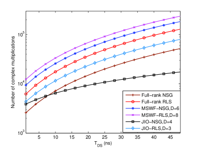
Figure 2: Number of multiplications required for different algorithms.

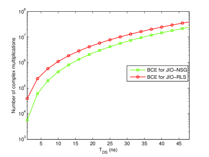
Figure 3: Number of multiplications required for BCEs.

VI-B Rank Adaptation

In the proposed blind JIO reduced-rank receiver, the computational complexity and the performance are sensitive to the determined rank $D$. In this section, a rank adaptation algorithm is employed to achieve better tradeoffs between the performance and the complexity of the JIO receiver. The rank adaptation algorithm is based on the a posteriori LS cost function to estimate the MSE, which is a function of $\bar{\mathbf{w}}_{D}(i)$ and $\mathbf{T}_{D}(i)$ and can be expressed as

$$\mathscr{C}_{D}(i)=\sum^{i}_{n=0}\lambda_{D}^{i-n}\left(|\bar{\mathbf{w}}_{D}^{H}(n)\mathbf{T}_{D}^{H}(n)\mathbf{r}(n)|^{2}-1\right)^{2},$$ (57)

where $\lambda_{D}$ is a forgetting factor. Since the optimal rank can be considered as a function of the time interval $i$ [19], the forgetting factor is required and allows us to track the optimal rank. For each time instant, we update a transformation matrix $\mathbf{T}_{\rm M}(i)$ and a reduced-rank filter $\bar{\mathbf{w}}_{\rm M}(i)$ with the maximum rank $D_{\rm max}$, which can be expressed as

$$\begin{split}&\mathbf{T}_{\rm M}(i)=[\mathbf{t}_{\rm M,1}(i),\dots,\mathbf{t}_{\rm M,\it D}(i),\dots,\mathbf{t}_{\rm M,\it D_{\rm max}}(i)]^{T}\\ &\bar{\mathbf{w}}_{\rm M}(i)=[\bar{w}_{\rm M,1}(i),\dots,\bar{w}_{\rm M,\it D}(i),\dots,\bar{w}_{\rm M,\it D_{\rm max}}(i)]^{T}\\ \end{split}$$ (58)

After the adaptation, we test values of $D$ within the range $D_{\rm min}$ to $D_{\rm max}$. For each tested rank, we use the following estimators

$$\begin{split}&\mathbf{T}_{D}(i)=[\mathbf{t}_{\rm M,1}(i),\dots,\mathbf{t}_{\rm M,\it D}(i)]^{T}\\ &\bar{\mathbf{w}}_{D}(i)=[\bar{w}_{\rm M,1}(i),\dots,\bar{w}_{\rm M,\it D}(i)]^{T}\\ \end{split}$$ (59)

and substitute (59) into (57) to obtain the value of $\mathscr{C}_{D}(i)$, where $D\in\{D_{\rm min},\ldots,D_{\rm max}\}$. The proposed algorithm can be expressed as

$$D_{\rm opt}(i)=\arg\min_{D\in\{D_{\rm min},\ldots,D_{\rm max}\}}\mathscr{C}_{D}(i).$$ (60)

We remark that the complexity of updating the reduced-rank filter and the transformation matrix in the proposed rank adaptation algorithm is the same as the receiver with rank $D_{\rm max}$, since we only adapt the $\mathbf{T}_{\rm M}(i)$ and $\bar{\mathbf{w}}_{\rm M}(i)$ for each time instant. However, additional computations are required for calculating the values of $\mathscr{C}_{D}(i)$ and selecting the minimum value of a $(D_{\rm max}-D_{\rm min}+1)$-dimensional vector that corresponds to a simple search and comparison.

VII Simulations

In this section, the proposed NSG and RLS versions of the blind JIO adaptive receivers are applied to the uplink of a multiuser BPSK DS-UWB system. The performance of the proposed receivers are compared with the RAKE receiver with the maximal-ratio combining (MRC), the NSG and RLS versions of the full-rank schemes and the MSWF. Note that, the blind channel estimation described in section III is implemented to provide channel coefficients to the RAKE receiver and its bit-error rate (BER) performance is averaged for the purpose of comparison. In all simulations, all the users are assumed to be transmitting continuously at the same power level. The pulse shape adopted is the RRC pulse with the pulse-width $0.375$ns. The spreading codes are generated randomly for each user with a spreading gain of $32$ and the data rate of the communication is approximately $83$Mbps. We assess the blind receivers with the standard IEEE 802.15.4a channel models of channel model 1 (ChMo1) and channel model 2 (ChMo2), which are for indoor residential line-of-sight (LOS) and non-line of sight (NLOS) environments, respectively. [41]. We assume that the channel is constant during the whole transmission. The channel delay spread is $T_{DS}$ = 10ns and the ISI from 2 neighbor symbols are taken into account for the simulations. The sampling rate at the receiver is assumed to be 2.67GHz and the length of the discrete time received signal is M = 59. For all the experiments, all the adaptive receivers are initialized as vectors with all the elements equal to 1. This allows a fair comparison between the analyzed techniques for their convergence performance. In practice, the filters can be initialized with prior knowledge about the spreading code or the channel to accelerate the convergence. In all the simulations, the phase of $h(0)$ is used as a reference to remove the phase ambiguity derived from the blind channel estimates. All the curves shown in this section are obtained by averaging 200 independent runs. In this section, the coded bit error rate (BER) performances are obtained by adopting a convolutional code with a coding-rate of 2/3. The code polynomial is [7,5,5] and the constraint length is set to 5. It should be noted that other coding schemes employing Turbo codes, LDPC codes and/or iterative detection [45] can be employed to further improve the performance of the proposed algorithms.

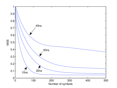
Figure 4: MSE performance of the blind channel estimation (with ChMo2).

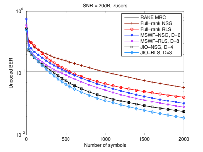
Figure 5: Uncoded BER performance of different algorithms with ChMo2. For full-rank NSG: $\mu=0.025$, full-rank RLS: $\delta=10$, $\lambda=0.9998$. For MSWF-NSG, $D=6$, $\mu=0.025$; MSWF-RLS: $D=8$, $\lambda=0.998$. For JIO-NSG $D=4$, $c_{max}=3$, $v=1$, $\mu_{T,0}=0.075$, $\mu_{w,0}=0.005$; JIO-RLS: $D=3$, $\lambda=0.9998$, $\delta=10$, $v=0.5$.

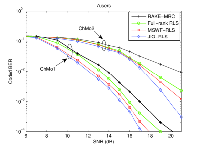
Figure 6: BER performance of the proposed scheme with different SNRs.

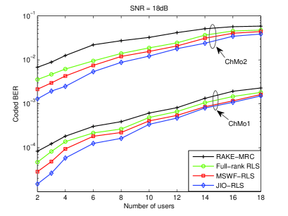
Figure 7: BER performance of the proposed scheme with different number of users.

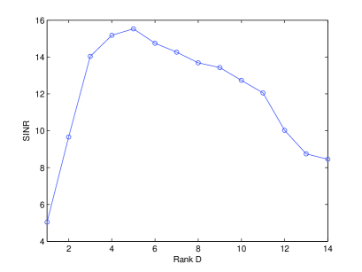
Figure 8: SINR performance with different rank D (with ChMo2).

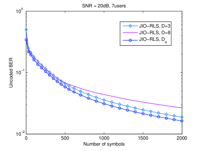
Figure 9: Uncoded BER performance of the rank-adaptation algorithm (with ChMo2).

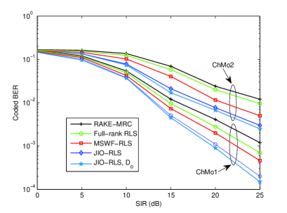
Figure 10: BER performance of the adaptive algorithm with NBI. For NBI, $f_{d}=23MHz$.

Firstly, we access the mean squared error (MSE) performance of the blind channel estimator that is introduced in section III with the ChMo2. As shown in Fig.4, the MSE performance is shown as a function of number of transmitted symbols with different channel delays in a 7-user scenario with a signal-to-noise ratio (SNR) of 20dB. The performance of the blind channel estimation is highly dependent on the channel delays. The performance of the CCM-based blind adaptive algorithms will be degraded significantly in the scenarios of large channel delays due to the inaccuracy of the blind channel estimation. In this work, we consider a channel delay of 10ns.

In Fig.5, we compare the uncoded BER performance of the proposed JIO receivers with the full-rank NSG and RLS algorithms, the MSWF-NSG and MSWF-RLS in the NLOS environment (ChMo2). In a 7-user scenario with a SNR of 20dB, the uncoded BER performance of different algorithms as a function of symbols transmitted is presented that enables us to compare the convergence rate of different adaptive algorithms. Among all the analyzed algorithms, the proposed JIO-RLS algorithm converges fastest. The JIO-NSG algorithm outperforms the MSWF versions and the full-rank versions with a low complexity. A noticeable improvement on the BER performance is obtained by using the JIO receivers.

In Fig.6 and Fig. 7, we access the coded BER performances of the blind algorithms with different SNRs in a $7$-user scenario and with different numbers of users in a 18dB SNR scenario, respectively. Both ChMo1 and ChMo2 are considered in these simulations. The parameters set for all the adaptive algorithms are the same as in Fig.5. The proposed JIO versions show better MAI and ISI canceling capability in all the simulated scenarios. It can be observed that the use of channel coding improves the performance of the receivers and that the same hierarchy in terms of BER performance is verified - the proposed JIO-RLS algorithm achieves the best performance. In Fig.6, the JIO-RLS can save around 2dB in comparison with the MSWF-RLS with ChMo2 for a BER around $10^{-3}$ and save around 1dB with ChMo1 for a BER around $10^{-4}$. In Fig.7, the JIO-RLS scheme can support more than 2 additional users in comparison with the MSWF-RLS with ChMo2 for a BER around $10^{-3}$ and can support over 1 additional users with ChMo1 for a BER around $10^{-4}$.

In Fig.8, the signal to interference plus noise ratio (SINR) performance is shown as a function of rank D in the NLOS environment (ChMo2). We consider a 7-user scenario with a SNR of 20dB. A noticeable better performance is obtained for the ranks in the range of 3 to 8. In this scenario, D = 5 performs best and a 1.5dB gain is achieved compare to the algorithm with D = 3 and D = 8. Note that, for the JIO-RLS algorithm, the complexity is $O(DM^{2})$. The designer can choose the rank D as a parameter that will affect the complexity and the performance.

Fig.9 compares the uncoded BER performance in the NLOS environment (ChMo2) of the JIO-RLS using the rank-adaptation algorithm given by (60) with $D_{\rm max}=8$ and $D_{\rm min}=3$. The results using a fixed-rank of 3 and 8 are also shown for comparison purposes and illustration of the sensitivity of the JIO scheme to the rank D. The forgetting factor is $\lambda_{D}=0.998$. It can be seen that the uncoded BER performance of the JIO-RLS scheme with the rank-adaptation algorithm outperforms the fixed-rank scenarios with $D_{\rm min}=3$ and $D_{\rm max}=8$. In this experiment, $D=3$ has better steady state performance than $D=8$, with both cases showing the similar convergence speed. The rank-adaptation algorithm provides a better solution than the fixed rank approaches. It should be noted that the complexity of updating the transformation matrix and the reduced-rank filter in the rank adaptation algorithm is the same as the fixed rank case with $D=D_{\rm max}$. Additional complexity is required to compute the values of $\mathscr{C}_{D}(i)$ by using (57) and select the minimum value of a $(D_{\rm max}-D_{\rm min}+1)$-dimensional vector.

In the last experiment, we examine the blind adaptive algorithms with an additional narrow band interference (NBI), which is modeled as a single-tone signal (complex baseband) [50]:

$$J(t)=\sqrt{P_{j}}e^{\left(2\pi f_{d}t+\theta_{j}\right)},$$ (61)

where $P_{j}$ is the NBI power, $f_{d}$ is the frequency difference between the carrier frequency of the UWB signal and the one of the NBI and $\theta_{j}$ is the random phase which is uniformly distributed in $[0,\pi)$. Here, the received signal can be expressed as

$$z(t)=\sum_{k=1}^{K}\sum_{l=0}^{L-1}h_{k,l}x^{(k)}(t-lT_{\tau})+n(t)+J(t).$$ (62)

Note that, in this experiment, the receivers are required to suppress the ISI, MAI and NBI together blindly. In Fig. 10, in a 5-user system with a 18dB SNR, the coded BER performance of the RLS versions are compared with different signal to NBI ratio (SIR) with ChMo1 and ChMo2. The algorithms are set the same parameters as in Fig.5. With the NBI, the eigenvalue spread of the covariance matrix of the received signal is increased and this change slows down the convergence rate of the full-rank scheme. However, the proposed JIO receiver shows better ability to cope with this change and the performance gain over the full-rank scheme is increased compared to the NBI free scenarios. By adopting the rank adaptation algorithm, the performance is improved as compared to the fixed rank JIO-RLS receiver in the simulated scenarios. This is mainly because of the faster convergence speed that is introduced by the rank adaptation algorithm.

VIII Conclusions

A novel blind reduced-rank receiver is proposed based on JIO and the CCM criterion. The novel receiver consists of a transformation matrix and a reduced-rank filter. The NSG and RLS adaptive algorithms are developed for updating its parameters. In DS-UWB systems, both versions (NSG and RLS) of the proposed blind reduced-rank receivers outperform the analyzed CCM based full-rank and existing reduced-rank adaptive schemes with a low complexity. The robustness of the proposed receivers has been demonstrated in the scenario that the blind receivers are required to suppress the ISI, MAI and NBI together. The proposed blind receivers can be employed in spread-spectrum systems which encounter large filter problems and suffer from severe interferences.

Appendix A Convergence Properties

In this section, we examine the convergence properties of the cost function $\mathbf{J}_{\rm JIO}=\frac{1}{2}E\left[(\left|y(i)\right|^{2}-1)^{2}\right]$, where $y(i)=\bar{\mathbf{w}}^{H}(i)\mathbf{T}^{H}(i)\mathbf{r}(i)$. For simplicity of the following analysis, we drop the time index $(i)$. The received signal is given by

$$\begin{split}\mathbf{r}&=\sum_{k=1}^{K}\sqrt{E_{k}}\mathbf{P}_{r}\mathbf{S}_{e,k}\mathbf{h}_{k}b_{k}+\mbox{\boldmath$\eta$}+\mathbf{n},\\ &=\sum_{k=1}^{K}\sqrt{E_{k}}b_{k}\mathbf{p}_{k}+\mbox{\boldmath$\eta$}+\mathbf{n}=\mathbf{P}_{k}\mathbf{A}_{k}\mathbf{b}+\mbox{\boldmath$\eta$}+\mathbf{n},\end{split}$$ (63)

where $\mathbf{p}_{k}=\mathbf{P}_{r}\mathbf{S}_{e,k}\mathbf{h}_{k}$, $k=1,\dots,K$, are the signature vectors of the users. $\mathbf{P}_{k}=[\mathbf{p}_{1},\dots,\mathbf{p}_{K}]$, $\mathbf{A}_{k}=diag(\sqrt{E_{1}},\dots,\sqrt{E_{K}})$ and $\mathbf{b}=[b_{1},\dots,b_{K}]$. $\eta$ and $\mathbf{n}$ represent the ISI and AWGN, respectively. We assume that $b_{k}$, $k=1,\dots,K$, are statistically independent i.i.d random variables with zero mean and unit variance and are independent to the noises. Firstly, we will discuss the noise-free scenario for the analysis, in which, the output signal of the JIO receiver is given by

$$y=\bar{\mathbf{w}}^{H}\mathbf{T}^{H}\mathbf{P}_{k}\mathbf{A}_{k}\mathbf{b}=\mbox{\boldmath$\epsilon$}^{H}\mathbf{b},$$ (64)

where $\mbox{\boldmath$\epsilon$}\triangleq\mathbf{A}_{k}^{H}\mathbf{P}_{k}^{H}\mathbf{T}\bar{\mathbf{w}}=[\mbox{$\epsilon$}_{1},\dots,\mbox{$\epsilon$}_{K}]$. Assuming that user 1 is the desired user and recalling the constraint $\bar{\mathbf{w}}^{H}\mathbf{T}^{H}\mathbf{p}_{1}=v$, where $v$ is a real-valued constant. We obtain that the first element of the vector $\epsilon$ can be expressed as

$$\mbox{$\epsilon$}_{1}=\sqrt{E_{1}}\mathbf{p}_{1}^{H}\mathbf{T}\bar{\mathbf{w}}=\sqrt{E_{1}}v.$$ (65)

Now, let us have a closer look at the cost function,

$$\begin{split}\mathbf{J}_{\rm JIO}&=\frac{1}{2}E\left[\left|y(i)\right|^{4}-2\left|y(i)\right|^{2}+1\right]\\ &=\frac{1}{2}\left(E\left[(\mbox{\boldmath$\epsilon$}^{H}\mathbf{b}\mathbf{b}^{H}\mbox{\boldmath$\epsilon$})^{2}\right]-2E\left[\mbox{\boldmath$\epsilon$}^{H}\mathbf{b}\mathbf{b}^{H}\mbox{\boldmath$\epsilon$}\right]+1\right)\\ &=\frac{1}{2}\left(\sum^{K}_{k=1}\sum^{K}_{j=1}|\mbox{$\epsilon$}_{k}|^{2}|\mbox{$\epsilon$}_{j}|^{2}|b_{k}|^{2}|b_{j}|^{2}-2\sum^{K}_{k=1}|\mbox{$\epsilon$}_{k}|^{2}|b_{k}|^{2}+1\right)\\ &=\frac{1}{2}\left(\sum^{K}_{k=1}\sum^{K}_{j=1}|\mbox{$\epsilon$}_{k}|^{2}|\mbox{$\epsilon$}_{j}|^{2}-2\sum^{K}_{k=1}|\mbox{$\epsilon$}_{k}|^{2}+1\right)\\ &=\frac{1}{2}(|\mbox{$\epsilon$}_{1}|^{2}+\tilde{\mbox{\boldmath$\epsilon$}}^{H}\tilde{\mbox{\boldmath$\epsilon$}})^{2}-(|\mbox{$\epsilon$}_{1}|^{2}+\tilde{\mbox{\boldmath$\epsilon$}}^{H}\tilde{\mbox{\boldmath$\epsilon$}})+\frac{1}{2}\\ \end{split}$$ (66)

where $\tilde{\mbox{\boldmath$\epsilon$}}=[\mbox{$\epsilon$}_{2},\dots,\mbox{$\epsilon$}_{k}]=\tilde{\mathbf{A}}_{k}^{H}\tilde{\mathbf{P}}_{k}^{H}\mathbf{T}\bar{\mathbf{w}}$, $\tilde{\mathbf{P}}_{k}=[\mathbf{p}_{2},\dots,\mathbf{p}_{K}]$ and $\tilde{\mathbf{A}}_{k}=diag(\sqrt{E_{2}},\dots,\sqrt{E_{K}})$. Equation (66) transforms the cost function of both $\mathbf{T}$ and $\bar{\mathbf{w}}$ into a function with single variable $\tilde{\mbox{\boldmath$\epsilon$}}$. We remark that $\tilde{\mbox{\boldmath$\epsilon$}}$ is a linear function of $\mathbf{T}\bar{\mathbf{w}}$ that is the blind reduced-rank receiver. Hence, the convexity properties of the cost function with respect to $\tilde{\mbox{\boldmath$\epsilon$}}$ reflects the convexity properties of the cost function with respect to $\mathbf{T}\bar{\mathbf{w}}$. To evaluate the convexity of $\mathbf{J}_{\rm JIO}$, we compute its Hessian that is given by

$$\mathbf{H}_{JIO}=\frac{\partial}{\partial\tilde{\mbox{\boldmath$\epsilon$}}^{H}}\frac{\partial\mathbf{J}_{\rm JIO}}{\partial\tilde{\mbox{\boldmath$\epsilon$}}}=2\tilde{\mbox{\boldmath$\epsilon$}}\tilde{\mbox{\boldmath$\epsilon$}}^{H}+(|\mbox{$\epsilon$}_{1}|^{2}-1)\mathbf{I}.$$ (67)

It can be concluded that a sufficient condition for $\mathbf{H}_{JIO}$ to be a positive definite matrix is $|\mbox{$\epsilon$}_{1}|^{2}>1$, which is $E_{1}v^{2}>1$. This condition is obtained in noiseless scenario, however, it also holds for small $\sigma^{2}$ that can be considered as a slight perturbation of the noise-free case [10]. For larger values of $\sigma^{2}$, the term $v$ can be adjusted to ensure the convexity of the cost function.

References

- [1] M. Z. Win and R. A. Scholtz, “Impulse radio: how it works,” IEEE Comms. letters, vol. 2, no. 2, pp. 36-38, Feb. 1998.
- [2] L. Yang and G.B. Giannakis, “Ultra-wideband communications: an idea whose time has come,” IEEE Signal Processing Mag., vol. 21, no. 6, pp. 26-54, Nov. 2004.
- [3] R. C. Qiu, H. P. Liu and X. Shen, “Ultra-wideband for multiple access,” IEEE Commun. Mag., vol. 43, no. 2, pp. 80-87, Feb. 2005.
- [4] X. Dong, J. Li and P. Orlik, “A new transmitted reference pulse cluster system for UWB communications,” IEEE Trans. Vehicular Technology, vol. 57, no. 5, pp. 3217-3224, Sept. 2008.
- [5] M. Wolf, N. Song and M. Haardt, “Non-Coherent UWB Communications,” FREQUENZ Journal of RF-Engineering and Telecommun., special issue on Ultra-Wideband Radio Technologies for Commun., Localisation and Sensor applications, vol. 63,pp. 187-191, Oct. 2009.
- [6] I. Oppermann, M. Hamalainen and J. Iinatti, UWB Theory and Applications, John Wiley, 2004.
- [7] D. Cassioli, M. Z. Win, F. Vatalaro and A. F. Molisch, “Low complexity rake receivers in ultra-wideband channels,” IEEE Trans. Wireless Commun., vol. 6, no. 4, pp. 1265-1275, Apr. 2007.
- [8] M. Honig, U. Madhow and S. Verdu, “Blind adaptive multiuser detection,” IEEE Trans. Inform. Theory, vol. 49, no. 9, pp. 1642-1648, Sept. 2001.
- [9] R. C. de Lamare and R. Sampaio-Neto, “Low-Complexity Variable Step-Size Mechanisms for Stochastic Gradient Algorithms in Minimum Variance CDMA Receivers,” IEEE Trans. Signal Process., vol. 54, no. 6, pp. 2302-2317, Jun. 2006.
- [10] C. Xu, G. Feng and K. S. Kwak, “A Modified Constrained Constant Modulus Approach to Blind Adaptive Multiuser Detection,” IEEE trans. Commun., vol. 49, no. 9, pp. 1642-1648, Sept. 2001.
- [11] R. C. de Lamare and R. Sampaio-Neto, “Blind Adaptive Code-Constrained Constant Modulus Algorithms for CDMA Interference Suppression in Multipath Channels,” IEEE Comms. letters, vol. 9, no. 4, pp. 334-336, Apr. 2005.
- [12] R. C. de Lamare, M. Haardt and R. Sampaio-Neto, “Blind Adaptive Constrained Reduced-Rank Parameter Estimation Based on Constant Modulus Design for CDMA Interference Suppression,” IEEE Trans. Signal Process., vol. 56, no. 6, pp. 2470-2482, Jun. 2008.
- [13] P. Liu, and Z. Xu, “Blind MMSE-Constrained Multiuser Detection,” IEEE Trans. Vehicular Technology, vol. 57, no. 1, pp. 608-615, Jan. 2008.
- [14] J. Miguez and L. Castedo, “A Linearly Constrained Constant Modulus Approach to Blind Adaptive Multiuser Interference Suppression,” IEEE Comms. letters, vol. 2, no. 8, pp. 217-219, Aug. 1998.
- [15] G. S. Biradar, S. N. Merchant and U. B. Desai, “ Performance of Constrained Blind Adaptive DS-CDMA UWB Multiuser Detector in Multipath Channel with Narrowband Interference ,” IEEE GLOBECOM 2008, pp. 1-5 , Dec. 2008.
- [16] J. Liu and Z. Liang, “Linearly Constrained Constant Modulus Algorithm Based Blind Multi-User Detection for DS-UWB Systems,” IEEE WiCom 2007, pp. 578-581 , Sept. 2007.
- [17] A. M. Haimovich and Y. Bar-Ness, “An eigenanalysis interference canceler,” IEEE Trans. Signal Process., vol. 39, no. 1, pp. 76-84, Jan. 1991.
- [18] J. S. Goldstein and I. S. Reed, “Reduced-rank adaptive filtering,” IEEE Trans. Signal Process., vol. 45, no. 2, pp. 492-496, Feb. 1997.
- [19] M. L. Honig and J. S. Goldstein, “Adaptive reduced-rank interference suppression based on the multistage wiener filter,” IEEE Trans. Commun., vol. 50, no. 6, pp. 986-994, Jun. 2002.
- [20] J. D. Hiemstra, Robust Implementations of the Multistage Wiener Filter, PhD. thesis of Virginia Polytechnic Institute and State University, Apr. 2003.
- [21] J. S. Goldstein,I. S. Reed, and L. L. Scharf, “A multistage representation of the Wiener filter based on orthogonal projections,” IEEE Trans. Information Theory, vol. 44, no. 11, pp. 2943-2959, Nov. 1998.
- [22] W. Chen, U. Mitra and P. Schniter, “On the equivalence of three reduced rank linear estimators with applications to DS-CDMA,” IEEE Trans. on Information Theory, vol. 48, no. 9, pp. 2609-2614, Sep. 2002.
- [23] L. Wang and R. C. de Lamare, “Constrained adaptive filtering algorithms based on conjugate gradient techniques for beamforming,” IET Signal Processing, 2010.
- [24] D. A. Pados and G. N. Karystinos, “An iterative algorithm for the computation of the MVDR filter,” IEEE Trans. Signal Process., vol. 49, no. 2, pp. 290-300, Feb. 2001.
- [25] R. C. de Lamare and R. Sampaio-Neto, “Adaptive Reduced-Rank MMSE Filtering with Interpolated FIR Filters and Adaptive Interpolators”, IEEE Sig. Proc. Letters, vol. 12, no. 3, March, 2005.
- [26] R. C. de Lamare and R. Sampaio-Neto, “Reduced-rank adaptive filtering based on joint iterative optimization of adaptive filters,” IEEE Signal Process. lett., vol. 14, no. 12, pp. 980-983, Dec. 2007.
- [27] R. C. de Lamare, “Adaptive reduced-rank LCMV beamforming algorithms based on joint iterative optimisation of filters,” Electronics Letters, vol. 44, pp. 565-566, Apr. 2008.
- [28] R. C. de Lamare, L. Wang, and R. Fa, “Adaptive reduced-rank LCMV beamforming algorithms based on joint iterative optimization of filters: Design and analysis,” Elsevier Signal Processing, vol. 90, pp. 640-652, Feb. 2010.
- [29] R. C. de Lamare and R. Sampaio-Neto, “Adaptive Reduced-Rank Processing Based on Joint and Iterative Interpolation, Decimation, and Filtering,” IEEE Transactions on Signal Processing, vol. 57, no. 7, July 2009, pp. 2503 - 2514.
- [30] R.C. de Lamare, R. Sampaio-Neto, M. Haardt, ”Blind Adaptive Constrained Constant-Modulus Reduced-Rank Interference Suppression Algorithms Based on Interpolation and Switched Decimation,” IEEE Transactions on Signal Processing, vol.59, no.2, pp.681-695, Feb. 2011.
- [31] R. C. de Lamare and R. Sampaio-Neto, “Reduced-Rank Space-Time Adaptive Interference Suppression With Joint Iterative Least Squares Algorithms for Spread-Spectrum Systems,” IEEE Transactions on Vehicular Technology, vol.59, no.3, March 2010, pp.1217-1228.
- [32] R.C. de Lamare and R. Sampaio-Neto, “Adaptive Reduced-Rank Equalization Algorithms Based on Alternating Optimization Design Techniques for MIMO Systems,” IEEE Trans. Vehicular Technology, vol. 60, no. 6, pp.2482-2494, July 2011.
- [33] J. Zhang, T. D. Abhayapala and R. A. Kennedy, “Principal components tracking algorithms for synchronization and channel identification in UWB systems,” IEEE Eighth International Symposium on Spread Spectrum Techniques and Applications (ISSSTA), pp. 369-373, Sept. 2004.
- [34] S. H. Wu, Y. S. Cheng and S. C. Kuo, “Multistage MMSE receivers for ultra-wide bandwidth impulse radio communications,” International Workshop on Ultra Wideband Systems, Joint with Conference on Ultrawideband Systems and Technologies. pp. 16-20, May. 2004.
- [35] Z. Tian, H. Ge and L. L. Scharf, “Low-complexity multiuser detection and reduced-rank Wiener filters for ultra-wideband multiple access,” IEEE International Conference on Acoustics, Speech, and Signal Processing (ICASSP), vol. 3, pp. 621-624, Mar. 2005.
- [36] Y. Tian and C. Yang, “Reduced-order Multiuser Detection in Multi-rate DS-UWB Communications,” IEEE International Conf. on Commun.(ICC), vol.10, pp. 4746-4750, Jun. 2006.
- [37] S. Li and R. C. de Lamare “Low-complexity Reduced-Rank Interference Mitigation Algorithms for DS-UWB Systems,” IEEE Vehicular Technology Conference (VTC), May. 2010.
- [38] Z. Xu, P. Liu and J. Tang, “A Subspace Approach to BlindMultiuser Detection for Ultra-Wideband Communication Systems,” EURASIP Journal on Applied Signal Processing: Special Issue on UWB - State of the Art, vol. 2005, no. 3, pp. 413-425, Mar. 2005.
- [39] R. Fisher, R. Kohno, M. McLaughlin, and M. Welbourn, “DS-UWB Physical Layer Submission to IEEE 802.15 Task Group 3a (Doc. Number P802.15-04/0137r4),” IEEE P802.15, Jan. 2005.
- [40] A. Parihar, L. Lampe, R. Schober, and C. Leung, “Equalization for DS-UWB systems–Patr I: BPSK modulation,” IEEE Trans. Commun., vol. 55, no. 6 pp. 1164-1173, Jun. 2007.
- [41] A. F. Molisch et al., “IEEE 802.15.4a Channel Model - Final Report,” Tech. Rep. Doc. IEEE 802.15-0400662-02-004a, 2005.
- [42] A. F. Molisch et al., “A Comprehensive Standardized Model for Ultrawideband Propagation Channels,” IEEE Trans. Antennas and propagation, vol. 54, no. 11, pp. 3151-3166, Nov. 2006.
- [43] X. G. Doukopoulos and G. V. Moustakides, “Adaptive power techniques for blind channel estimation in CDMA systems,” IEEE Trans. Signal Process. vol. 53, no. 3, pp. 1110-1120, Mar. 2005.
- [44] S. Haykin, Adaptive Filter Theory, Fourth Edition, Pearson Education, 2002.
- [45] R. C. de Lamare and R. Sampaio-Neto, “Minimum Mean-Squared Error Iterative Successive Parallel Arbitrated Decision Feedback Detectors for DS-CDMA Systems,” IEEE Trans. Commun., vol. 56, no. 5 pp. 778-789, May. 2007.
- [46] Y. Cai and R. C. de Lamare, ”Adaptive Space-Time Decision Feedback Detectors with Multiple Feedback Cancellation”, IEEE Transactions on Vehicular Technology, vol. 58, no. 8, October 2009, pp. 4129 - 4140.
- [47] R. Fa, R. C. de Lamare, ”Multi-branch successive interference cancellation for MIMO spatial multiplexing systems: Design, analysis and adaptive implementation,” IET Communications, vol.5, no.4, pp.484-494, March 2011.
- [48] P. Li, R. C. de Lamare and R. Fa, “Multiple Feedback Successive Interference Cancellation Detection for Multiuser MIMO Systems,” IEEE Transactions on Wireless Communications, vol. 10, no. 8, pp. 2434-2439, August 2011.
- [49] P. Li and R. C. de Lamare, “Adaptive Decision Feedback Detection with Constellation Constraints for MIMO Systems”, IEEE Transactions on Vehicular Technology, 2012.
- [50] X. Chu and R. D. Murch, “The effect of NBI on UWB time-hopping systems,” IEEE Trans. Wireless Commun. vol. 3, no. 5, pp. 1431-1436, Sept. 2004.