Guaranteed convergence of the Kohn–Sham equations

Abstract

A sufficiently damped iteration of the Kohn–Sham equations with the exact functional is proven to always converge to the true ground-state density, regardless of the initial density or the strength of electron correlation, for finite Coulomb systems. We numerically implement the exact functional for one-dimensional continuum systems and demonstrate convergence of the damped KS algorithm. More strongly correlated systems converge more slowly.

Kohn–Sham density functional theory (KS-DFT) Kohn and Sham (1965) is a widely applied electronic structure method. Standard approximate functionals yield accurate ground-state energies and electron densities for many systems of interest Burke (2012), but often fail when electrons are strongly correlated. Ground-state properties can be qualitatively incorrect Mori-Sánchez et al. (2009), and convergence can be very slow Daniels and Scuseria (2000); Thogersen et al. (2004). To remedy this, several popular schemes augment Kohn–Sham theory, such as LDA+U Anisimov et al. (1997). Others seek to improve approximate functionals Heyd et al. (2003) within the original formulation. But what if the exact functional does not exist for strongly correlated systems? Even if it does, what if the method fails to converge? Either plight would render KS-DFT useless for strongly correlated systems, and render fruitless the vast efforts currently underway to treat e.g., oxide materials Assmann et al. (2013), with KS-DFT.

The Kohn–Sham (KS) approach employs a fictitious system of non-interacting electrons, defined to have the same density as the interacting system of interest. The potential characterizing this KS system is unique if it exists Hohenberg and Kohn (1964). Because the KS potential is a functional of the density, in practice one must search for the density and KS potential together using an iterative, self-consistent scheme Dreizler and Gross (1990). The converged density is in principle the ground-state density of the original, interacting system, whose ground-state energy is a functional of this density.

Motivated by concerns of convergence and existence, we have been performing KS calculations with the exact functional for one-dimensional (1d) continuum systems Stoudenmire et al. (2012); Wagner et al. (2012). Even when correlations are strong, we never find a density whose KS potential does not exist, consistent with the results of Ref. Chayes et al. (1985). Nor do we find any system where the KS scheme does not converge, although convergence can slow by orders of magnitude as correlation is increased, just as in approximate calculations Daniels and Scuseria (2000); Thogersen et al. (2004).

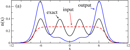
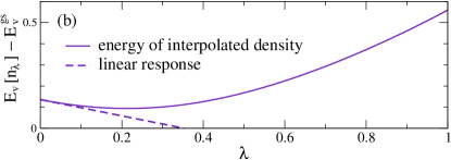
Figure 1: (a) The input and output densities for a single step of the Kohn–Sham scheme, as well as the exact density, of a one-dimensional, strongly correlated 4 atom, 4 electron system. (b) The energy of the system which interpolates between the input and output densities, $E_{v}[n_{\lambda}]$, measured from the ground-state energy $E^{\text{gs}}_{v}$. Also shown is the linear-response approximation with slope given by Eq. (12).

Exact statements about the unknown density functional inform the construction of all successful DFT approximations Levy and Perdew (1985); Perdew et al. (1996); Perdew and Kurth (2003); Perdew et al. (2005). More importantly, they distinguish between what a KS-DFT calculation can possibly do, and what it cannot. The most notorious example is the demonstration that the KS band-gap of a semiconductor does not equal the true charge gap, even when the exact functional is used Perdew et al. (1982); Stoudenmire et al. (2012). Our key result is an analytic proof that a simple algorithm guarantees convergence of the KS equations for all systems, weakly or strongly correlated, independent of the starting point. Thus multiple stationary points and failures to converge are artifacts of approximate functionals. Studies of convergence are well-known in applied mathematics; but almost all concern simple approximations, such as LDA Anantharaman and Cancès (2009), Hartree-Fock Cancès and Le Bris (2000), etc., and not those in current use in many calculations.

The basic idea lies in a single step of the KS scheme, which proceeds from an input density to produce an output density. For a strongly correlated system as in Fig. 1.a, the output density can differ strongly from the input density, and be further from the true ground-state density. Nevertheless, by proving that the initial slope is always negative as in Fig. 1.b, we show there is always a linear combination of the input and output densities that lowers the energy. By sufficiently damping each KS step, the energy is always reduced each iteration, yielding the ground-state density and energy to within a given tolerance in a finite number of iterations.

The KS algorithm is designed to minimize the energy as a functional of the electron density, $n({\bf r})$. For an $N$-electron system with a reasonable external potential $v({\bf r})$, the energy functional is Kohn and Sham (1965):

$$E_{v}[n]=T_{\scriptscriptstyle\rm S}[n]+\int d^{3}r\,n({\bf r})\,v({\bf r})+E_{\scriptscriptstyle\rm HXC}[n],$$ (1)

where $T_{\scriptscriptstyle\rm S}[n]$ is the kinetic energy of non-interacting (NI) electrons having density $n({\bf r})$, and $E_{\scriptscriptstyle\rm HXC}[n]$ is the Hartree-exchange-correlation (HXC) energy Lieb (1983); Fiolhais et al. (2003). The KS equations are, in atomic units,

$$-\frac{1}{2}\nabla^{2}\phi_{j}({\bf r})+\Big{(}v({\bf r})+v_{\scriptscriptstyle\rm HXC}[n]({\bf r})\Big{)}\phi_{j}({\bf r})=\epsilon_{j}\,\phi_{j}({\bf r}),$$ (2)

where $v_{\scriptscriptstyle\rm HXC}[n]({\bf r})=\delta E_{\scriptscriptstyle\rm HXC}[n]/\delta n({\bf r})$ is the HXC potential, $\phi_{j}({\bf r})$ are the electron orbitals, and $\epsilon_{j}$ their eigenvalues. (In this work, we consider spin-unpolarized systems for simplicity.) An output density $n^{\prime}({\bf r})$ is found by doubly occupying the lowest-energy orbitals:

$$n^{\prime}({\bf r})=2\sum_{j=1}^{\infty}f_{j}\,|\phi_{j}({\bf r})|^{2},$$ (3)

where $0\leq f_{j}\leq 1$ and $\sum_{j}f_{j}=N/2$. Fractional occupation is only allowed for the highest occupied orbitals if they are degenerate, where $f_{j}$ is chosen to minimize the difference between $n({\bf r})$ and $n^{\prime}({\bf r})$ .

Consider convergence of the following simple algorithm. Given an input density $n({\bf r})$, solve the KS equations to obtain the output density $n^{\prime}({\bf r})$. Define

$$\eta\equiv\dfrac{1}{N^{2}}\int d^{3}r\,\big{(}n^{\prime}({\bf r})-n({\bf r})\big{)}^{2}.$$ (4)

Choose some small $\delta>0$, and if $\eta<\delta$, then the calculation has converged. Otherwise, the next input is

$$n_{\lambda}({\bf r})=(1-\lambda)\,n({\bf r})+\lambda\,n^{\prime}({\bf r}),$$ (5)

for some $\lambda\in(0,1]$, and repeat. An ensemble-$v$-representable $n({\bf r})$ is the ground-state density (or an ensemble mixture of degenerate ground-state densities) for some local potential $v[n]({\bf r})$ Levy (1982); van Leeuwen (2003). For NI electrons, this potential is $v_{\scriptscriptstyle\rm S}[n]({\bf r})$. We call $n({\bf r})$ physical when both potentials exist, and we require all $n_{\lambda}({\bf r})$ to be physical. We refer to a single iteration of Eqs. (2)-(5) as one step of the KS algorithm. Taking full steps with $\lambda=1$ does not usually lead to a fixed point. But taking damped steps with $\lambda<1$ ensures the algorithm converges, as we now prove.

Lemma.–Consider two finite systems of $N$ electrons, with ground-state densities $n({\bf r})$, $n^{\prime}({\bf r})$, and potentials $v[n]({\bf r})\neq v[n^{\prime}]({\bf r})$, by which we mean the potentials differ by more than a constant. Then Hohenberg and Kohn (1964)

$$\int d^{3}r\,\Big{(}v[n^{\prime}]({\bf r})-v[n]({\bf r})\Big{)}\big{(}n^{\prime}({\bf r})-n({\bf r})\big{)}<0.$$ (6)

Proof.–Following Ref. Hohenberg and Kohn (1964), we apply the variational principle. Since $n({\bf r})$ is the ground-state density of the potential $v[n]({\bf r})$, we have $E_{v[n]}[n]<E_{v[n]}[n^{\prime}]$, or

$$\int d^{3}r\,v[n]({\bf r})\big{(}n({\bf r})-n^{\prime}({\bf r})\big{)}<F[n^{\prime}]-F[n],$$ (7)

where $F[n]\equiv T_{\scriptscriptstyle\rm S}[n]+E_{\scriptscriptstyle\rm HXC}[n]$. It is also true that $E_{v[n^{\prime}]}[n^{\prime}]<E_{v[n^{\prime}]}[n]$, so we may switch primes with unprimes in Eq. (7). Adding the resulting equation to the original yields Eq. (6). $\square$ Note that the lemma is true for any interaction between electrons, including none.

Theorem.–Given an arbitrary physical density $n({\bf r})$ as input into the KS algorithm,

$$E_{v}^{\prime}[n]\equiv\left.\dfrac{dE_{v}[n_{\lambda}]}{d\lambda}\right|_{\lambda=0}\leq 0,$$ (8)

where $n_{\lambda}({\bf r})$ is defined as in Eq. (5). If equality holds, then $n({\bf r})$ is a stationary point of $E_{v}[n]$.

Proof.–Consider $\Delta E_{v}$ resulting from $\lambda\,\Delta n({\bf r})$ $\equiv\lambda\,\big{(}n^{\prime}({\bf r})-n({\bf r})\big{)}$ $=n_{\lambda}({\bf r})-n({\bf r})$. Then

$$E_{v}^{\prime}[n]=\int d^{3}r\,\left.\dfrac{\delta E_{v}[n]}{\delta n({\bf r})}\right.\Delta n({\bf r}).$$ (9)

For a physical density, the functional derivative is van Leeuwen (2003)

$$\dfrac{\delta E_{v}[n]}{\delta n({\bf r})} = -v_{\scriptscriptstyle\rm S}[n]({\bf r})+v({\bf r})+v_{\scriptscriptstyle\rm HXC}[n]({\bf r}).$$ (10)

Since $v({\bf r})+v_{\scriptscriptstyle\rm HXC}[n]({\bf r})$ defines $v_{\scriptscriptstyle\rm S}[n^{\prime}]({\bf r})$ ($n^{\prime}({\bf r})$ is the output density of Eq. (2)), we have:

$$\left.\dfrac{\delta E_{v}[n]}{\delta n({\bf r})}\right.=v_{\scriptscriptstyle\rm S}[n^{\prime}]({\bf r})-v_{\scriptscriptstyle\rm S}[n]({\bf r}).$$ (11)

Combining Eq. (11) and Eq. (9) gives:

$$E_{v}^{\prime}[n]=\int d^{3}r\,\Big{(}v_{\scriptscriptstyle\rm S}[n^{\prime}]({\bf r})-v_{\scriptscriptstyle\rm S}[n]({\bf r})\Big{)}\,\big{(}n^{\prime}({\bf r})-n({\bf r})\big{)}.$$ (12)

Two cases arise: if $v_{\scriptscriptstyle\rm S}[n^{\prime}]({\bf r})\neq v_{\scriptscriptstyle\rm S}[n]({\bf r})$, use the lemma applied to NI systems: then $E_{v}^{\prime}[n]$ must be less than zero. Otherwise, $v_{\scriptscriptstyle\rm S}[n^{\prime}]({\bf r})=v_{\scriptscriptstyle\rm S}[n]({\bf r})$, so both $E_{v}^{\prime}[n]$ and the RHS of Eq. (11) are zero, and $n({\bf r})$ is a stationary point of $E_{v}[n]$. $\square$ We illustrate the theorem in Fig. 1.b, where we plot $E_{v}[n_{\lambda}]$ and its linear-response approximation for the input density of Fig. 1.a.

Corollary 1.–The KS algorithm described above is guaranteed to converge to a stationary point of the functional, if (1) only physical densities are encountered, (2) the energy functional is convex, and (3) appropriate values for $\lambda$ are used, e.g. from the algorithm of Ref. Birgin et al. (2003), because it is effectively a gradient-descent algorithm .

Corollary 2.–When using the exact functional, the KS algorithm using appropriate $\lambda$’s converges to the exact ground-state density, as long as the first input density is a physical density. This is because we can choose each subsequent input density as a physical density , and the exact ensemble-functional Valone (1980); Lieb (1983) is convex. The only stationary point of the exact functional, when considering physical densities, is the ground-state density Perdew and Levy (1985).

Numerical implementation.–To find the KS energy functional exactly when there is no degeneracy, we must find the many-electron wavefunction $\Psi[n]$ that minimizes $\langle\Psi|{\hat{T}}+{\hat{V}}_{\rm ee}|\Psi\rangle$ (the kinetic and electron-electron repulsion energies) with density $n({\bf r})$ Levy (1979); Lieb (1983). To perform this very demanding Schuch and Verstraete (2009) interacting inversion, start with a guess for the potential, $\tilde{v}({\bf r})$. Then solve the many-body system for the ground-state wavefunction $\tilde{\Psi}$ and density $\tilde{n}({\bf r})$. Using a quasi-Newton method Broyden (1965), modify $\tilde{v}({\bf r})$ and repeat, minimizing the difference between $\tilde{n}({\bf r})$ and the target density $n({\bf r})$. Once converged, the procedure is repeated for NI electrons. The HXC energy is then

$$E_{\scriptscriptstyle\rm HXC}[n]=\langle\Psi[n]|{\hat{T}}+{\hat{V}}_{\rm ee}|\Psi[n]\rangle-T_{\scriptscriptstyle\rm S}[n],$$ (13)

and the HXC potential is

$$v_{\scriptscriptstyle\rm HXC}[n]({\bf r})=v_{\scriptscriptstyle\rm S}[n]({\bf r})-v[n]({\bf r}).$$ (14)

We implement these functionals for 1d continuum systems Stoudenmire et al. (2012); Wagner et al. (2012), obtaining highly-accurate many-body solutions with the density matrix renormalization group White (1992, 1993). These are the first such inversions for systems with more than 2 electrons Thiele et al. (2008); Coe et al. (2009). Because, in 1d, degeneracy (beyond spin) does not occur, we find pure states $\Psi[n]$. More generally, one should invert using an ensemble $\Gamma[n]$ and take a trace in Eq. (13) Valone (1980); Lieb (1983).

Figure 2: KS procedure for a moderately correlated 4-electron system (four hydrogen atoms with $R=3$), showing the first few iterations. Using a fixed $\lambda=0.30$, we converge to $\eta<10^{-6}$ using Eq. (4) within 13 iterations.

To illustrate convergence of the damped KS algorithm using the exact functional, we plot the output densities and KS potentials for a four-electron, four-atom system in Fig. 2. We choose the interatomic spacing $R=3$ to be roughly twice the equilbrium spacing of H₂ (when the interaction between nuclei is the same as that between electrons), making this a moderately correlated system. Taking $\lambda=0.30$, the algorithm converges to the exact density (computed separately using DMRG) to $\eta<10^{-6}$ using Eq. (4), within 13 steps.

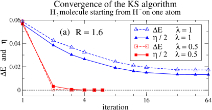
Figure 3: Differences in the density $\eta$ using Eq. (4) and the energy with $\Delta E=E_{v}[n^{\prime}]-E^{\text{gs}}_{v}$, for an H₂ molecule with (a) $R=1.6$ and (b) $R=3$. In (b), the $\Delta E$ curves are omitted for clarity, but are like those in (a).

Consider the KS scheme applied to a simple 1d H₂ molecule with bond length $R$ Wagner et al. (2012). Initialize the algorithm with an asymmetric input density, an H^- density centered on the left atom. Of course, no sensible KS calculation starts with such a density, but we do this to amplify convergence issues. In Fig. 3, we quantify the convergence of the KS algorithm using $\eta$ from Eq. (4) as well as energy differences from the ground-state. For the equilibrium bond length ($R=1.6$), $\lambda$ may be chosen quite large ($\approx 0.5$); but as the atoms are stretched to $R=3$, $\lambda$ must be $\lesssim 0.2$. When $R=5$, even $\lambda=0.01$ is too large to converge the calculation (not shown). Thus, as the bond is stretched and the system develops strong static correlation Wagner et al. (2012), convergence becomes increasingly difficult. As more atoms are added to the chain (not shown), such as stretched H₄, even a reasonable initial state converges very slowly.

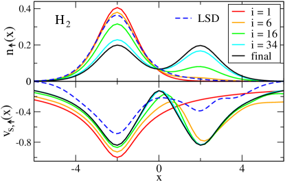
Figure 4: Starting an exact KS calculation of stretched H₂ with a spin-polarized density still converges (with $\lambda=0.5$) to the correct spin-singlet density. For the same initial density, the KS calculation with the local spin-density (LSD) approximation Helbig et al. (2011) converges to the broken spin-symmetry solution.

Consequences for real calculations.–For approximate XC functionals, the corresponding $E_{v}[n]$ is not, in general, convex for every $v({\bf r})$, and our corollaries do not hold. Consider H₂ in the local spin-density approximation. At and near equilibrium bond lengths, only one stationary solution exists. The approximate functional may or may not be convex. But when the bond is stretched beyond the infamous Coulson–Fischer point Coulson and Fischer (1949); Perdew et al. (1995), an unrestricted solution of lower energy appears Wagner et al. (2012), as in Fig. 4, so the corresponding $E_{v}[n]$ is not convex and convergence with our simple algorithm is not guaranteed. While the restricted solution is a saddle point, the unrestricted solution is a local minimum. Thus, only the unrestricted solution behaves locally like the solution with the exact functional, providing further rationale Perdew et al. (1995) for preferring such a solution over any restricted one. On the other hand, slowing of convergence as correlations become stronger is a real effect, and not an artifact of approximations.

We chose our simple algorithm to prove convergence, but many are more sophisticated and efficient (see e.g. Daniels and Scuseria (2000); Thogersen et al. (2004)). Mixing KS potentials instead of densities Kerker (1981) can similarly be proven to converge, with the advantage that all densities encountered are NI $v$-representable.

Finally, we expect that orbital degeneracies in 3d require the ensemble treatment Valone (1980); Levy (1982); Lieb (1983); Ullrich and Kohn (2001). Further, extending the KS approach to use fractional occupation of electron orbitals (even in the case of non-degeneracy) may speed convergence Rabuck and Scuseria (1999) and allow KS-DFT to more naturally handle strong static correlation Schipper et al. (1998).

The authors acknowledge DOE grant DE-SC0008696, and LW also thanks the Korean global research network grant (No. NRF-2010-220-C00017). LW thanks Stefano Pittalis, Marcos Raydan, Robert van Leeuwen and Mel Levy for helpful discussions.

References

- Kohn and Sham (1965) W. Kohn and L. J. Sham, “Self-consistent equations including exchange and correlation effects,” Phys. Rev. 140, A1133–A1138 (1965).
- Burke (2012) K. Burke, “Perspective on density functional theory,” J. Chem. Phys. 136 (2012).
- Mori-Sánchez et al. (2009) Paula Mori-Sánchez, Aron J. Cohen, and Weitao Yang, “Discontinuous nature of the exchange-correlation functional in strongly correlated systems,” Phys. Rev. Lett. 102, 066403 (2009).
- Daniels and Scuseria (2000) Andrew D. Daniels and Gustavo E. Scuseria, “Converging difficult scf cases with conjugate gradient density matrix search,” Phys. Chem. Chem. Phys. 2, 2173–2176 (2000).
- Thogersen et al. (2004) Lea Thogersen, Jeppe Olsen, Danny Yeager, Poul Jorgensen, Pawel Salek, and Trygve Helgaker, “The trust-region self-consistent field method: Towards a black-box optimization in hartree–fock and kohn–sham theories,” The Journal of Chemical Physics 121, 16–27 (2004).
- Anisimov et al. (1997) Vladimir I Anisimov, F Aryasetiawan, and A I Lichtenstein, “First-principles calculations of the electronic structure and spectra of strongly correlated systems: the lda + u method,” Journal of Physics: Condensed Matter 9, 767 (1997).
- Heyd et al. (2003) Jochen Heyd, Gustavo E. Scuseria, and Matthias Ernzerhof, “Hybrid functionals based on a screened coulomb potential,” The Journal of Chemical Physics 118, 8207–8215 (2003), ibid. 124, 219906(E) (2006).
- Assmann et al. (2013) Elias Assmann, Peter Blaha, Robert Laskowski, Karsten Held, Satoshi Okamoto, and Giorgio Sangiovanni, “Oxide heterostructures for efficient solar cells,” Phys. Rev. Lett. 110, 078701 (2013).
- Hohenberg and Kohn (1964) P. Hohenberg and W. Kohn, “Inhomogeneous electron gas,” Phys. Rev. 136, B864–B871 (1964).
- Dreizler and Gross (1990) R. M. Dreizler and E. K. U. Gross, Density Functional Theory: An Approach to the Quantum Many-Body Problem (Springer–Verlag, Berlin, 1990).
- Stoudenmire et al. (2012) E. M. Stoudenmire, Lucas O. Wagner, Steven R. White, and Kieron Burke, “One-dimensional continuum electronic structure with the density-matrix renormalization group and its implications for density-functional theory,” Phys. Rev. Lett. 109, 056402 (2012).
- Wagner et al. (2012) Lucas O. Wagner, E.M. Stoudenmire, Kieron Burke, and Steven R. White, “Reference electronic structure calculations in one dimension,” Phys. Chem. Chem. Phys. 14, 8581 – 8590 (2012).
- Chayes et al. (1985) J.T. Chayes, L. Chayes, and MaryBeth Ruskai, “Density functional approach to quantum lattice systems,” Journal of Statistical Physics 38, 497–518 (1985).
- Levy and Perdew (1985) M. Levy and J.P. Perdew, “Hellmann-feynman, virial, and scaling requisites for the exact universal density functionals. shape of the correlation potential and diamagnetic susceptibility for atoms,” Phys. Rev. A 32, 2010 (1985).
- Perdew et al. (1996) John P. Perdew, Kieron Burke, and Matthias Ernzerhof, “Generalized gradient approximation made simple,” Phys. Rev. Lett. 77, 3865–3868 (1996), ibid. 78, 1396(E) (1997).
- Perdew and Kurth (2003) John P. Perdew and Stefan Kurth, “Density functionals for non-relativistic Coulomb systems in the new century,” in A Primer in Density Functional Theory, edited by Carlos Fiolhais, Fernando Nogueira, and Miguel A. L. Marques (Springer, Berlin / Heidelberg, 2003) pp. 1–55.
- Perdew et al. (2005) John P. Perdew, Adrienn Ruzsinszky, Jianmin Tao, Viktor N. Staroverov, Gustavo E. Scuseria, and Gabor I. Csonka, “Prescription for the design and selection of density functional approximations: More constraint satisfaction with fewer fits,” The Journal of Chemical Physics 123, 062201 (2005).
- Perdew et al. (1982) John P. Perdew, Robert G. Parr, Mel Levy, and Jose L. Balduz, “Density-functional theory for fractional particle number: Derivative discontinuities of the energy,” Phys. Rev. Lett. 49, 1691–1694 (1982).
- Anantharaman and Cancès (2009) Arnaud Anantharaman and Eric Cancès, “Existence of minimizers for kohn–sham models in quantum chemistry,” Annales de l’Institut Henri Poincare (C) Non Linear Analysis 26, 2425 – 2455 (2009).
- Cancès and Le Bris (2000) Eric Cancès and Claude Le Bris, “On the convergence of scf algorithms for the hartree-fock equations,” ESAIM: Mathematical Modelling and Numerical Analysis 34, 749–774 (2000).
- Note (1) The precise restrictions on potentials are detailed in Ref. Lieb (1983); Coulomb potentials are allowed.
- Lieb (1983) Elliott H. Lieb, “Density functionals for coulomb systems,” Int. J. Quantum Chem. 24, 243–277 (1983).
- Fiolhais et al. (2003) Carlos Fiolhais, F. Nogueira, and M. Marques, A Primer in Density Functional Theory (Springer-Verlag, New York, 2003).
- Note (2) An orbital rotation among degenerate orbitals may also be required; see Ref. Ullrich and Kohn (2001).
- Ullrich and Kohn (2001) C. A. Ullrich and W. Kohn, “Kohn-sham theory for ground-state ensembles,” Phys. Rev. Lett. 87, 093001 (2001).
- Levy (1982) Mel Levy, “Electron densities in search of hamiltonians,” Phys. Rev. A 26, 1200–1208 (1982).
- van Leeuwen (2003) Robert van Leeuwen, “Density functional approach to the many-body problem: Key concepts and exact functionals,” (Academic Press, 2003) pp. 25 – 94.
- Note (3) We restrict our attention to finite systems, since in an extended system Eq. (6\@@italiccorr) would be ill defined.
- Birgin et al. (2003) Ernesto G. Birgin, José Mario Martínez, and Marcos Raydan, “Inexact spectral projected gradient methods on convex sets,” IMA Journal of Numerical Analysis 23, 539–559 (2003).
- Note (4) With respect to gradient descent minimization, we assume that functionals behave like their less dimensionful counterparts, functions. A more comprehensive analysis is beyond the scope of this work.
- Note (5) In the language of DFT, we can find an ensemble--representable density which is arbitarily close to a density which has reasonable properties: integrating to a finite particle number , with a finite von Weizsäcker kinetic energy, i.e. , and being nowhere negative Lieb (1983); van Leeuwen (2003). This set of reasonable densities is convex van Leeuwen (2003); so that is reasonable if both and are, which is the case. The examples of Ref. Englisch and Englisch (1983) are not in this set.
- Englisch and Englisch (1983) H. Englisch and R. Englisch, “Hohenberg-Kohn theorem and non-V-representable densities,” Physica A: Statistical Mechanics and its Applications 121, 253 – 268 (1983).
- Valone (1980) Steven M. Valone, “A one-to-one mapping between one-particle densities and some n-particle ensembles,” The Journal of Chemical Physics 73, 4653–4655 (1980).
- Perdew and Levy (1985) John P. Perdew and Mel Levy, “Extrema of the density functional for the energy: Excited states from the ground-state theory,” Phys. Rev. B 31, 6264–6272 (1985).
- Levy (1979) Mel Levy, “Universal variational functionals of electron densities, first-order density matrices, and natural spin-orbitals and solution of the -representability problem,” Proceedings of the National Academy of Sciences of the United States of America 76, 6062–6065 (1979).
- Schuch and Verstraete (2009) Norbert Schuch and Frank Verstraete, “Computational complexity of interacting electrons and fundamental limitations of density functional theory,” Nat. Phys. 5, 732–735 (2009).
- Broyden (1965) C.G. Broyden, “A class of methods for solving nonlinear simultaneous equations,” Mathematics of Computation 19, 577–593 (1965).
- White (1992) Steven R. White, “Density matrix formulation for quantum renormalization groups,” Phys. Rev. Lett. 69, 2863 (1992).
- White (1993) Steven R. White, “Density-matrix algorithms for quantum renormalization groups,” Phys. Rev. B 48, 10345 (1993).
- Thiele et al. (2008) M. Thiele, E. K. U. Gross, and S. Kümmel, “Adiabatic approximation in nonperturbative time-dependent density-functional theory,” Phys. Rev. Lett. 100, 153004 (2008).
- Coe et al. (2009) J. P. Coe, K. Capelle, and I. D’Amico, “Reverse engineering in many-body quantum physics: Correspondence between many-body systems and effective single-particle equations,” Phys. Rev. A 79, 032504 (2009).
- Helbig et al. (2011) N. Helbig, J. I. Fuks, M. Casula, M. J. Verstraete, M. A. L. Marques, I. V. Tokatly, and A. Rubio, “Density functional theory beyond the linear regime: Validating an adiabatic local density approximation,” Phys. Rev. A 83, 032503 (2011).
- Coulson and Fischer (1949) C.A. Coulson and I. Fischer, “Xxxiv. notes on the molecular orbital treatment of the hydrogen molecule,” Philosophical Magazine Series 7 40, 386–393 (1949).
- Perdew et al. (1995) John P. Perdew, Andreas Savin, and Kieron Burke, “Escaping the symmetry dilemma through a pair-density interpretation of spin-density functional theory,” Phys. Rev. A 51, 4531–4541 (1995).
- Kerker (1981) G. P. Kerker, “Efficient iteration scheme for self-consistent pseudopotential calculations,” Phys. Rev. B 23, 3082–3084 (1981).
- Rabuck and Scuseria (1999) Angela D. Rabuck and Gustavo E. Scuseria, “Improving self-consistent field convergence by varying occupation numbers,” The Journal of Chemical Physics 110, 695–700 (1999).
- Schipper et al. (1998) P. R. T. Schipper, O. V. Gritsenko, and E. J. Baerends, “One - determinantal pure state versus ensemble kohn-sham solutions in the case of strong electron correlation: Ch2 and c2,” Theoretical Chemistry Accounts 99, 329–343 (1998).