Connecting Curves in Higher Dimensions

Abstract

Connecting curves have been shown to organize the rotational structure of strange attractors in three-dimensional dynamical systems. We extend the description of connecting curves and their properties to higher dimensions within the special class of differential dynamical systems. The general properties of connecting curves are derived and selection rules stated. Examples are presented to illustrate these properties for dynamical systems of dimension $n=3,4,5$.

I Introduction

Autonomous dynamical systems are defined by equations of the form $\dot{x}_{i}=f_{i}(x_{1},x_{2},\dots,x_{n})$, $i=1,2,\dots,n$. When a bounded attractor exists, its general structure is partly described by the location of the fixed points $\dot{x}_{i}=0$. Typically the fixed points are isolated. More information about the structure of an attracting set can be determined from the stability of each of the fixed points. The stability is determined from the eigenvalues of the jacobian $J_{ij}=\partial f_{i}/\partial x_{j}$ at each fixed point, and the eigenvectors associated with each eigenvalue.

When a dynamical system $\dot{x}_{i}=f_{i}$ generates a strange attractor, certain parts of the attractor “swirl” around one-dimensional invariant sets called connecting curvesGilmore10 . In such cases, connecting curves organize the global structure of the flow, and therefore provide more information than just the location and stability of the fixed points. Connecting curves defined by the eigenvalue-like condition $J_{ij}f_{j}=\lambda f_{i}$ have been studied in a number of three-dimensional dynamical systems. They are recognized as a kind of skeleton that helps to define the structure of a strange attractor.

In this work we explore the properties of connecting curves in dynamical systems of dimension $n\geq 3$. This is done in a restricted class of dynamical systems called differential dynamical systems. We describe the basic connectivity between fixed points and outline conditions that determine whether or not they lie on the connecting curve. We also describe the systematics of connecting curve attachment to or detachment from a fixed point and the recombinations or reconnections that can take place between different connecting curves.

Fixed points and their eigenvalue spectrum are used to predict changes in the local stability of a connecting curve as the control parameters are varied. Under certain conditions, we show that the global stability of a connecting curve can also be predicted. When the stability is such that the flow undergoes a swirling motion around the connecting curve, an integer index $\kappa$ is used to describe the swirling in terms of vortex or hypervortex structures. The formation of these structures plays an important role in determining the topology of strange attractors in higher dimensions.

In Sec. II we review the definition of connecting curves and their properties. The particular class of dynamical systems studied is introduced in Sec. III. In that Section we also describe how the distribution of fixed points in such systems is systematically organized by cuspoid catastrophes $A_{m}^{\prime}$, where $m$ is the maximum number of fixed points allowed by variation of the control parameters. We also describe how the stability properties of each fixed point are determined by another cuspoid catastrophe $A_{n}^{\prime}$, where $n$ is the dimension of the dynamical system. In Secs. IV, V, and VI we study cases of three-, four-, and five-dimensional dynamical systems with one, two, and three fixed points. These illustrate many of the properties of connecting curves described in Secs. II and III. Results are summarized in Sec. VII.

II Connecting Curves

Special points exist in the phase space $R^{n}$ of autonomous dynamical systems $\dot{x}_{i}=f_{i}(x)$ where the acceleration ${\bf\dot{f}}$ is proportional to the velocity ${\bf f}$. These points satisfy the eigenvalue equation ${\bf\dot{f}}=J{\bf f}=\lambda{\bf f}$, where $J=\partial f_{i}/\partial x_{j}$ is the jacobian. For an $n$-dimensional dynamical system, the equations represented by $J{\bf f}=\lambda{\bf f}$ provide $n$ constraints in an $n+1$ dimensional space $R^{n+1}$ consisting of $n$ phase space coordinates and one “eigenvalue”: $(x_{1},\dots,x_{n};\lambda)$. The intersections of the manifolds defined by these equations are one-dimensional sets in $R^{n+1}$ whose projection into the coordinate subspace $R^{n}$ is called a connecting curve.

Much like fixed points, connecting curves provide constraints on the behavior of local phase space trajectories. This behavior is determined by examining the eigenvalue spectrum of the jacobian matrix along the length of the connecting curve. The eigenvalues can occur in a variety of ways depending on the dimension, $n$, of the phase space: $n-2\kappa$ real and $\kappa$ complex conjugate pairs, with $\kappa=0,1,\cdots,[n/2]$.

Subsets of a connecting curve along which $\kappa=0$ are called strain curves because small volumes in their vicinity undergo irrotational deformation under the action of the flow. Deformation takes place along the principle stable and unstable directions indicated by the eigenvectors $\xi_{R}$ of the real eigenvalues $\lambda_{R}$.

In three dimensions $(n=3)$, subsets of the connecting curve along which $\kappa=1$ are known as vortex core curves. Vortex core curves were originally developed to identify vortices in complex hydrodynamic flowsRoth98 ; Peikert00 . They were later shown to organize the large-scale structure of strange attractors produced by three-dimensional dynamical systemsGilmore10 .

A vortex can be decomposed into its rotational and non-rotational components by linearizing the flow around its core curve. Rotation takes place on a plane spanned by the eigenvectors $\xi_{C}$ of the complex eigenvalues $\lambda_{C}$. The swirling flow is then transported along the eigenvector $\xi_{R}$ associated with the real eigenvalue $\lambda_{R}$. Under this combined action, trajectories are expected to undergo a tornado-like motion that spirals around the core in the direction of the flow.

The concept of a vortex can also be extended to higher dimensions in the phase space of dynamical systems. The basic idea is the same as in three-dimensions. Linearized flow around the core line is resolved into $\kappa\geq 1$ orthogonal planes of rotation that can be transported along $n-2\kappa$ directions. We refer to higher dimensional vortices with $\kappa\geq 2$ as hypervortices. Hypervortices and their associated core curves play an important role in organizing the large-scale structure of strange attractors in higher dimensions.

At a fixed point the initial conditions for a core curve are the eigenvectors with real eigenvalues. This observation has a number of important consequences. At a fixed point with $n-2\kappa$ real eigenvalues, $n-2\kappa$ connecting curves pass through the fixed point. This means that if $n-2\kappa=0$ at a fixed point, no connecting curves attach to the fixed point. If, under control parameter variation, the stability properties of a fixed point change when a pair of real eigenvalues become degenerate and transform to a complex conjugate pair, then two connecting curves must disconnect from the fixed point.

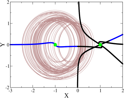
For the remainder of this work, we assign each of the connecting curve subsets a unique color. Strain curves ($\kappa=0$) are plotted in red, vortex core curves ($\kappa=1$) are plotted in black and hypervortex core curves ($\kappa=2$) are plotted in blue.

III Differential Dynamical Systems

We use differential dynamical systems to study connecting curves in higher dimensions for several reasons: (a) their canonical form has the same structure in all dimensions, (b) the jacobian matrix is simple and can be put into a Jordan-Arnol’d canonical form Arnold71 ; Gilmore81 when evaluated at the fixed points, and (c) only a single forcing function, $F(x_{1},x_{2},\cdots,x_{n-1},x_{n};c)$, needs to be modeled. Each of these properties is described in detail below.

III.1 The Canonical Form

Differential dynamical systems assume a canonical form in which each phase space coordinate except the first is the time derivative of the previous: $x_{i+1}=\dot{x}_{i}$

$$\begin{array}[]{lcl}\dot{x}_{1}&=&x_{2}\\ \dot{x}_{2}&=&x_{3}\\ &\vdots&\\ \dot{x}_{n-1}&=&x_{n}\\ \dot{x}_{n}&=&F(x_{1},x_{2},\cdots,x_{n-1},x_{n};c)\end{array}$$ (1)

This form is encountered when analyzing experimental data embedded using a differential embedding. Such embeddings are equivalent to Takens time-delay embeddings using a minimum time delay.

III.2 Fixed Points and Stability

The fixed points all lie along the $x_{1}$ axis because $\dot{x}_{i}=0\Rightarrow x_{i+1}=0$ for $i=1,2,\dots,n-1$. The stability properties of a fixed point at ${\bf x}_{f}=(x_{f},0\cdots,0,0)$ are determined by the eigenvalues of the jacobian matrix

$$J=\left[\begin{array}[]{cccccc}0&1&0&0&&0\\ 0&0&1&0&&0\\ &&&&\ddots&\\ 0&0&0&0&&1\\ F_{1}&F_{2}&F_{3}&F_{4}&&F_{n}\end{array}\right]_{{\bf x}_{f}}$$ (2)

evaluated at the fixed point ${\bf x}_{f}$, where as usual $F_{k}=\partial F/\partial x_{k}$. The secular equation for the eigenvalues at the fixed point is

$$\lambda^{n}-F_{n}\lambda^{n-1}\cdots-F_{2}\lambda^{1}-F_{1}\lambda^{0}=\lambda^{n}-\sum_{k=1}^{n}F_{k}\lambda^{k-1}=0$$ (3)

Setting $F_{n}=0$ converts the jacobian (2) into the Jordan-Arnol’d canonical form. In this form, the jacobian provides a standard unfolding for the cuspoid catastrophes $A_{n}$ which can be exploited to provide information about the stability properties of fixed points as the control parameters are varied Gilmore81 ; Thom76 ; Zeeman76 ; Poston78 .

III.3 Source Function

The canonical form (1) can be further simplified by making two assumptions about the nature of the single forcing function. We write the forcing function as the sum of two functions $F=G_{1}+G_{2}$

$$F(x_{1},\cdots,x_{n};c)=G_{1}(x_{1};c_{1})+G_{2}(x_{2},\cdots,x_{n};c_{2})$$ (4)

and split the control parameters $c$ for the original source function $F({\bf x};c)$ into two subsets, $c_{1}$ and $c_{2}$. The functions $G_{1}$ and $G_{2}$ satisfy the following properties.

$G_{1}$ is a function of only one variable, $x_{1}$, and control parameter set $c_{1}$. The fixed points are given by $G_{1}(x_{1};c_{1})=0$. Their number and location is controlled by the polynomial $G_{1}$ and the control parameters $c_{1}$. The term $F_{1}=G_{1}^{\prime}$ in the jacobian in Eq. (2). We choose $G_{1}$ to be a polynomial of degree $m$ with a maximum of $m$ real fixed points. In this work we take $m=1,2,3$ with a single control parameter $c_{1}=R$. The functions $G_{1}$ used in this work are outlined below.

For a maximum of one fixed point $(m=1)$ , we choose $G_{1}(x_{1};R)=Rx_{1}$. The fixed point is located at the origin and has slope $G^{{}^{\prime}}_{1}(x_{f})=R$.

For a maximum of two fixed points $(m=2)$, we chose $G_{1}(x_{1};R)=x_{1}^{2}-R$. There are no real fixed points for $R<0$, a doubly-degenerate fixed point for $R=0$ and two fixed points for $R>0$. The two real fixed points are created in a saddle-node bifurcation. They are symmetric and located at $x_{f_{1}}=-\sqrt{R}$ and $x_{f_{2}}=\sqrt{R}$ with slopes $G^{{}^{\prime}}_{1}(x_{f})=2x_{f}$, or $-2\sqrt{R}$ at $x_{f_{1}}$ and $+2\sqrt{R}$ at $x_{f_{2}}$.

For a maximum of three fixed points $(m=3)$, we choose $G_{1}(x_{1};R)=x_{1}^{3}-Rx_{1}$. There is one real fixed point for $R\leq 0$ and three for $R>0$. The three fixed points are created in a pitchfork bifurcation. One fixed point is located at the origin. The other two are at $x=\pm\sqrt{R}$. The critical points and their slopes are $(x_{f},G_{1}^{\prime}(x_{f})=(-\sqrt{R},2R);(0,-R);(+\sqrt{R},2R)$.

Along the $x_{1}$ axis the sign of $F_{1}=G_{1}^{\prime}$ alternates as successive fixed points are encountered. For fixed points with focal stability, this means an alternation of (stable focus - unstable outset) with (unstable focus - stable inset) along the $x$ axis. If $G_{1}^{\prime}>0$ at a fixed point then one eigenvalue is positive and the other two are negative, or have negative real part. If $G_{1}^{\prime}<0$ the reverse is true: one eigenvalue is negative and the other two are either positive or have positive real part. The net result is that if there are more than two fixed points, for an interior fixed point that is a stable focus with unstable outsets, the outsets can flow to the neighboring fixed points on its left and right, which are unstable foci with stable insets.

Figure 1: Bifurcation diagram created using a single Poincaré surface of section along the X-axis (Y=0) for Eq. (5) with $G_{1}(x,R)=x^{2}-R$. A period doubling route to chaos is observed after the saddle-node bifurcation at $R=0$. Parameter values: $(A,B)=(-1.7,-0.8)$.

$G_{2}$ is a function of the remaining variables, $x_{2},\cdots,x_{n-1},x_{n}$. Since the volume growth rate under the flow is determined by the divergence of the vector field, and the divergence is $\partial F/\partial x_{n}=\partial G_{2}/\partial x_{n}$, we impose the condition that $\partial G_{2}/\partial x_{n}$ is negative semi-definite throughout the phase space. Under such an assumption Eq. (1) describes a dissipative dynamical system.

The constant term in the Taylor series expansion of $G_{2}$ is zero. The linear terms $\sum_{j=2}^{n}a_{j}x_{j}$ define the terms $F_{j}$ that appear in the jacobian Eq. (2) when evaluated along the $x_{1}$ axis, specifically at fixed points: $F_{j}=a_{j}$, $j=2,\dots,n$. Thus, the stability of the fixed points is determined by the roots of the characteristic equation ${\rm det}(J-\lambda I_{n})=0$, given in Eq. (3). The center of gravity of the eigenvalues at a fixed point is $F_{n}=(G_{2})_{n}=a_{n}$. It is convenient to choose $a_{n}=0$ for two reasons. In this case all fixed points are unstable. Further, Eq. (3) assumes the form of the catastrophe function $G_{2}(x_{2},\dots,x_{n};s)|_{{\bf x}_{f_{j}}}=A_{n}^{\prime}(\lambda;a_{2},\dots,a_{n-1})$.

IV Three Dimensions

In this section we set $G_{2}(y,z;A,B)=Ay+Bzy^{2}$ in order to study three-dimensional differential dynamical systems that take the form

$$\begin{array}[]{l}\dot{x}=y\\ \dot{y}=z\\ \dot{z}=G_{1}(x;R)+Ay+Bzy^{2}\end{array}$$ (5)

The jacobian at any fixed point ${\bf x}_{f}$ is

$$J=\left[\begin{array}[]{ccc}0&1&0\\ 0&0&1\\ G_{1}^{\prime}&A&0\end{array}\right]_{{\bf x}_{f}}$$ (6)

with a characteristic polynomial

$${\rm det}(J-\lambda I_{3}))=A_{3}(\lambda)=\lambda^{3}-A\lambda-G_{1}^{\prime}(x_{f};R))$$ (7)

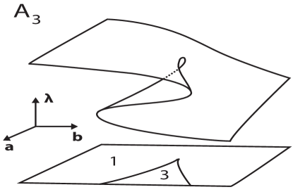
whose roots determine the stability properties (focus or saddle) of the fixed point. By making the substitution $(a,b)=(-A,-G_{1}^{\prime}(x_{f};R))$, (7) becomes the canonical unfolding of the cusp catastrophe $A_{3}$ whose bifurcation set is shown in Fig. 2(a). When projected down into the $(a,b)$ plane, the bifurcation set forms a well known cusp shape that divides the control parameter space into two regions. Inside the cusp, $(a/3)^{3}+(b/2)^{2}<0$ and the three eigenvalues of (6) are real. For control parameters in this region the fixed points of (5) have the stability of a saddle. Outside the cusp, $(a/3)^{3}+(b/2)^{2}>0$ and and the eigenvalues of (6) consist of one complex conjugate pair and one real. In this region, the fixed points have focal stability.

If $G_{1}^{\prime}=0$, the fixed point stability is determined along symmetry axis $b=0$. Outside the cusp ($a>0$), the fixed point is a center that has two complex conjugate eigenvalues with zero real part and a real eigenvalue that takes on a value of zero. Inside the cusp ($a<0$), the fixed point is a saddle and has three real eigenvalues. Two of the eigenvalues differ only by a sign. The third is equal to zero.

Connecting curves satisfy the following two constraints in the three-dimensional space $(x,y,\lambda)$ (c.f., Appendix 1)

$$\begin{array}[]{rcl}f(x,y,\lambda)&=&\lambda^{2}y\\ \left(G_{1}^{\prime}(x)+(B-2A\lambda y^{2})\lambda\right)y+\\ By^{2}f(x,y,\lambda)&=&\lambda f(x,y,\lambda)\end{array}$$ (8)

where $f(x,y,\lambda)=G_{1}(x)+Ay+B\lambda y^{3}$.

We use polynomials $G_{1}(x;R)$ of degree $m=2,3$ in the sections below to explore the spectrum of changes that can occur in the fixed points and connecting curves as the parameters $R$ and $B$ are varied.

IV.1 $m=2$

We begin by fixing $(A,B)=(-1.7,-0.8)$ and varying $R$ for $G_{1}(x_{1};R)=x^{2}-R$. A standard period-doubling route to chaos is observed in the bifurcation diagram shown in Fig. 1.

A pair of symmetry related fixed points are created in a saddle-node bifurcation as $R$ passes through zero. Their stability can be determined directly by evaluating the zeros of (7). A more convenient method is to examine the evolution of the fixed points in the catastrophe control parameter space $(a,b)=(-A,-2x_{f})$. This method allows us to predict the fixed point stability as the control parameters are changed. The fixed point stability for $R<0$ and $R=1$ is plotted in Fig. 2(b) using green dots. Their evolution as a function of $R$ is indicated by the green arrows.

No real fixed points exist for $R=-1$. Figure 3(a) shows that vortex and strain curves exist in the phase space despite the lack of fixed points. Phase space trajectories initialized near the core curve spiral along its length towards the right. These trajectories are unbounded.

(a) Bifurcation set for the cusp catastrophe $A_{3}$. The number of real eigenvalues in each region are indicated.

(b) Fixed point evolution for control parameters $(A,B)=(-1.7,-0.8)$ for $R<0$ and $R=1$ (center and outer pair)

(c) Fixed point evolution for control parameters $(B,R)=(-0.8,1)$ and $A=(1.0617,2.642,5.9012)$ (top to bottom)

Figure 2: Fixed point stability is determined by the coordinates $(a,b)=(-A,-2x_{f})$ in the $A_{3}$ catastrophe control parameter space. They are represented by the green circles. (b) The fixed points move along the $b$ axis as $R$ is varied. Since they remain outside the cusp region for all $R$, they will always have focal stability. (c) The fixed points move along the $a$ axis as $A$ is varied. The transition from outside to inside the cusp forces a transition in stability from focal to saddle. The governing equation is (5) using $G_{1}(x_{1};R)=x^{2}-R$.

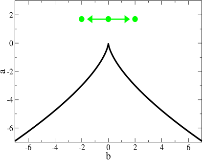
A real degenerate fixed point is created when $R=0$. It has coordinates $(a,b)=(1.7,0)$ in the catastrophe control parameter plane. Figure 2(b) shows that it is located directly above the cusp along the symmetry axis. Because it is both outside the cusp and on the symmetry axis, the fixed point is a center with a stable inset on the left and a unstable outset on the right. It appears on the vortex core curve in Fig. 3(b). Phase space trajectories spiral along the core curve towards the right and remain unbounded.

Two real fixed points are created as $R$ is increased past zero. As seen in Fig. 2(b), they move horizontally along the $b$ axis as $R$ is increased. Since the fixed point stability evolves outside of the cusp region for all $R\geq 0$, the fixed points always have focal stability for the current value of $A$. When $R=1$, the alternation of (stable focus - unstable outset) with (unstable focus - stable inset) builds up the strange attractor shown in Fig. 3(c).

(a) $R$ = -1

(b) $R$ = 0

(c) $R$ = 1

Figure 3: The connecting curves, fixed points and phase space trajectories are plotted in the X-Y plane for $R=(-1,0,1)$. The governing equation is (5) using $G_{1}(x_{1};R)=x^{2}-R$ with parameter values $(A,B)=(-1.7,-0.8)$. Fixed points undergo a saddle-node bifurcation as $R$ passes through zero. (a-b) Trajectories initialized near the vortex core line escape to infinity. (c) The alternating stability of the two fixed points creates conditions that generate a strange attractor.

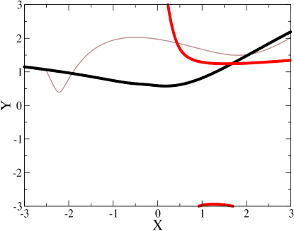
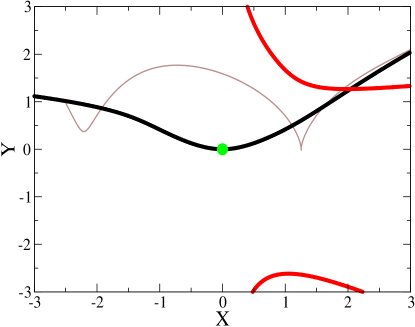
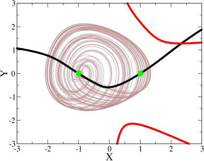
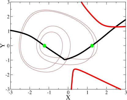
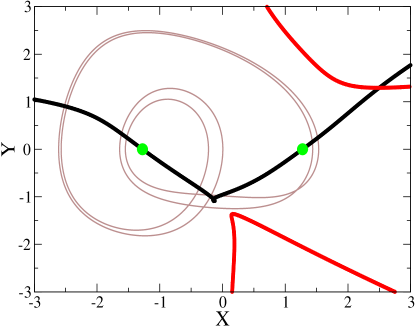
A reconnection between two connecting curves takes place as $R$ is increased past one. The sequence is shown in Fig. 4. The vortex core curve running between the two fixed points breaks and re-attaches itself with the strain curve approaching from the bottom. This sequence is important because it indicates that reconnections can be made between vortex and strain curves despite their different stability properties.

(a) $R$ = 1.5385

(b) $R$ = 1.6264

(c) $R$ = 1.7143

Figure 4: A reconnection between a vortex core curve and a strain curve is shown in the X-Y plane as $R$ is increased past one. The stable period four and period two orbits are shown in brown. The governing equation is (5) using $G_{1}(x_{1};R)=x^{2}-R$ with parameter values $(A,B)=(-1.7,-0.8)$.

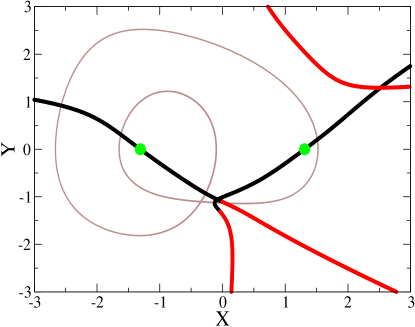
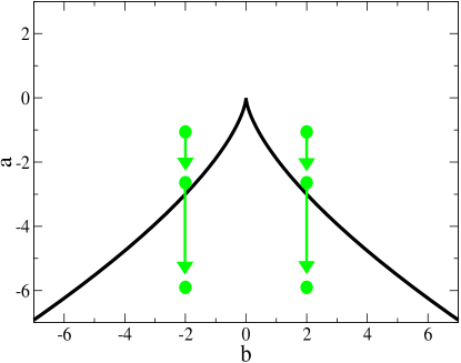
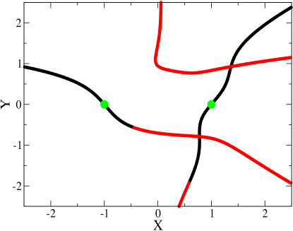
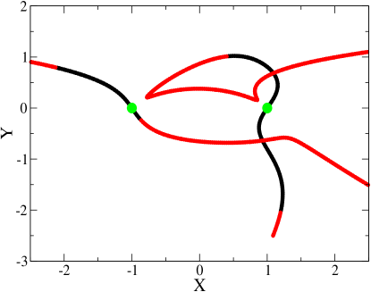
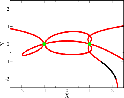
We end this sub-section by fixing the control parameters $(B,R)=(-0.8,1)$ and varying $A$. The fixed points now move along the $a$ axis and transition from outside to inside the cusp region. This transition is illustrated in Fig. 2(c) for three different values of $A$. The change from focal to saddle stability forces a corresponding change in stability along the connecting curve near the fixed point. When $a<-3$, all the eigenvalues become real and only strain curves can pass through the fixed points. The sequence in Fig. 5 shows the connecting curves during this transition.

(a) $A$ = 1.0617

(b) $A$ = 2.642

(c) $A$ = 5.9012

Figure 5: The connecting curve evolution is plotted in the X-Y plane as the parameter $A$ is varied. The changing stability of the fixed points force local changes in the stability of the connecting curves. The governing equation is (5) using $G_{1}(x_{1};R)=x^{2}-R$ with parameter values $(B,R)=(-0.8,1)$.

IV.2 $m=3$

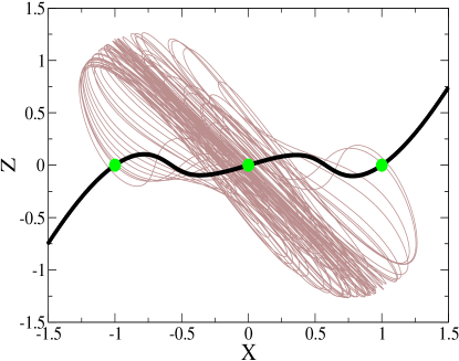
For $G_{1}(x_{1};R)=x^{3}-Rx$, the jacobian is given by Eq. (6) with $G_{1}^{\prime}(x_{1};R)=3x^{2}-R$. The description of the fixed point stability proceeds as in the case with $m=2$. The fixed point at the origin has coordinates $(a,b)=(-A,0)$ in the catastrophe control parameter plane. Because it sits on the symmetry axis, the fixed point is a center when $A<0$. For $A\geq 0$, it is a saddle. The symmetry related fixed points have the same coordinate $(a,b)=(-A,-2R)$ in the catastrophe control parameter plane. They have three real eigenvalues for $(a/3)^{3}<-R^{2}$. Otherwise, the fixed points have one real eigenvalue and a complex conjugate pair. Figure 6 shows the strange attractor, connecting curves and fixed points generated for parameter values $(A,B,R)=(-1.25,-0.8,1)$. The fixed point at the origin has two stable insets that attract flow along the vortex core curve from the two outer fixed points.

Figure 6: X-Z projection of the strange attractor generated by Eq. (5) with $G_{1}(x,R)=x^{3}-Rx$. The flow is organized by the fixed points and the vortex core curve. The fixed point at the origin is a center with stable insets. The symmetric fixed points are foci with unstable outsets. Parameter values: $(A,B,R)=(-1.25,-0.8,1)$.

V Four Dimensions

In this section we set $G_{2}(y,z,u;A,B,C)=Ay+Bz+Cu^{3}$ in order to study four-dimensional differential dynamical systems that take the form

$$\begin{array}[]{rcl}\dot{x}&=&y\\ \dot{y}&=&z\\ \dot{z}&=&u\\ \dot{u}&=&G_{1}(x;R)+Ay+Bz+Cu^{3}\end{array}$$ (9)

The jacobian at any fixed point ${\bf x}_{f}$ is

$$J=\left[\begin{array}[]{cccc}0&1&0&0\\ 0&0&1&0\\ 0&0&0&1\\ G_{1}^{\prime}&A&B&0\end{array}\right]_{{\bf x}_{f}}$$ (10)

with a characteristic polynomial

$${\rm det}(J-\lambda I_{4}))=A_{4}(\lambda)=\lambda^{4}-B\lambda^{2}-A\lambda-G_{1}^{\prime}(x_{f};R)$$ (11)

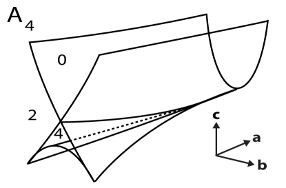
whose roots determine the stability properties of the fixed point. By making the substitution $(a,b,c)=(-B,-A,-G_{1}^{\prime}(x_{f};R))$, (11) becomes the canonical unfolding of the swallowtail catastrophe $A_{4}$ whose bifurcation set is shown in Fig. 7(a). The control parameter space is divided into three disjoint open regions that describe fixed points with four, two, or zero real eigenvalues and zero, one, or two pairs of complex conjugate eigenvalues. The open regions are connected and simply connected. The bifurcation sets separating these open regions satisfy $A_{4}(\lambda)=0$ and $dA_{4}(\lambda)/d\lambda=0$.

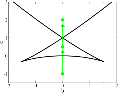
We use polynomials $G_{1}$ of degree $m=1,2,3$ in the sections below to study the properties of connecting curves in higher dimensions. For $m=1$, we set $B>0$ and vary the parameter $R$ such that the single fixed point traverses the three regions of stability shown in Fig. 7(b). We describe the effects on the connecting curves as the fixed point passes through each of the regions. We also determine the global stability of the connecting curve as a function of the single phase space variable $u$.

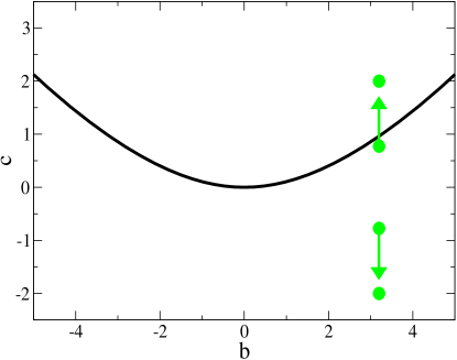
For $m=2,3$ we set $B<0$ such that the control parameter space is divided into two regions where (10) produces one or two pairs of complex conjugate eigenvalues. Under certain conditions, the fixed points can assume different values of the index $\kappa$. We describe these effects on the structure of strange attractors and their connecting curves.

(a) Bifurcation set for the swallowtail catastrophe $A_{4}$. The number of real eigenvalues in each region are indicated.

(b) Cross section of the bifurcation set taken at $a=-2$. The fixed point evolution is shown for $(A,B,C)=(0,2,-1)$ and $R=(1,-0.5,-2)$ (bottom to top)

(c) Cross section of the bifurcation set taken at $a=2.335$. The fixed point evolution is shown for $(A,B,C)=(-3.2,-2.335,-1)$ and $R=(0.15,1)$ (center to outer pair)

Figure 7: Fixed point stability is determined by the coordinates $(a,b,c)$ in the $A_{4}$ catastrophe control parameter space. They are represented by the green circles. (b) The single fixed point for $G_{1}(x_{1};R)=Rx$ moves through the three regions of stability as $R$ is varied. (c) The two real fixed point for $G_{1}(x_{1};R)=x^{2}-R$ move through the two regions of stability as $R$ is varied.

V.1 $m=1$

To investigating the global stability of connecting curves change in higher dimensions, we fix $(A,B,C)=(0,2,-1)$ and vary $R$ for $G_{1}(x_{1};R)=Rx$. The stability of the single fixed point at the origin depends on its coordinates $(a,b,c)=(-2,0,-R)$ in the catastrophe control parameter space. As $R$ is varied, the fixed point moves along the symmetry axis $(b=0)$ and passes through the three regions of stability shown in Fig. 7(b). Along the symmetry axis, the fixed point has the following eigenvalue spectrum: one degenerate complex conjugate eigenvalue pair when $c<0$; none for $0<c<(a/2)^{2}$; and a doubly degenerate pair for $c>(a/2)^{2}$.

Although useful, the fixed points only provide limited (local) information about the stability of a connecting curve. The stability of an arbitrary point in phase space is determined by the characteristic equation of the jacobian evaluated at that point. For the control parameters listed above, the characteristic equation is

$${\rm det}(J-\lambda I_{4}))=C_{p}(\lambda,u;R)=\lambda^{4}+3u^{2}\lambda^{3}-2\lambda^{2}-R$$ (12)

which is a function of the single phase space variable $u$. Equation (12) is used to create a simple partition of the phase space that determines the stability along the entire length of the connecting curve.

We start by choosing $R=1$ such that $c<0$. For this case the fixed point has a degenerate complex conjugate eigenvalue pair. The index $\kappa=1$. The $n-2\kappa=2$ vortex core curves that pass through the fixed point are shown in Fig. 8(a). Equation (12) produces a single pair of complex conjugate eigenvalues for all $u$. As a result, the global stability properties of the connecting curve remain unchanged throughout the phase space.

Next, we set $R=-0.5$. This moves the fixed point into the region $0<c<(a/2)^{2}$ where no complex conjugate eigenvalue pairs are produced. Since $\kappa=0$, we expect $n-2\kappa=4$ strain curves to connect to the fixed point through all possible stable insets and unstable outsets. The strain curves for this value of $R$ are shown in Fig. 8(b). Using Eq. (12), the phase space is split into two parts. They are separated by the blue dotted line.

(a) $R=1$

(b) $R=-0.5$

(c) $R=-2$

Figure 8: Connecting curves and fixed point from Eq. (9) are plotted in the $X-U$ plane using $G_{1}(x,R)=Rx$ with parameter values $(A,B,C)=(0,2,-1)$. Equation (12) is used to partition the phase space (blue dotted line). These paritions define the stability of the connecting curves within them.

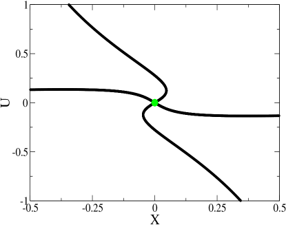
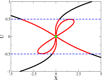
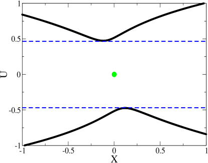
The first part of the phase space (center) contains only strain curves because (12) produces all real eigenvalues within this range of $u$. The second part of the phase space (top and bottom) contains only vortex core curves because (12) produces a single pair of complex conjugate eigenvalues. The abrupt change in stability that is observed to take place along the connecting curves is explained by a transition between the two phase space partitions.

Setting $R=-2$ moves the fixed point into the final region of the catastrophe control parameter space where $c>(a/2)^{2}$ and $\kappa=2$. In this region, $n-2\kappa=0$ connecting curves connect to the fixed point. The phase space is again divided into two parts using Eq. (12). The first part (center) produces two pairs of complex conjugate eigenvalues. No vortex core lines are able to enter this region. The second part (outer top and bottom) produces a single pair and supports the creation of vortex core lines as shown in Fig. 8(c).

V.2 $m=2$

For $m=2$ we fix the control parameters $(A,B,C)=(-3.2,-2.335,-1)$ and vary $R$ for $G_{1}(x_{1};R)=x^{2}-R$. A period doubling route to chaos is observed in Fig. 9.

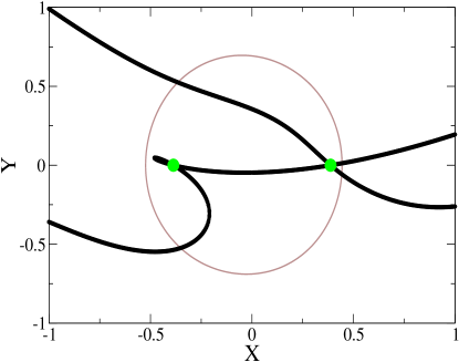
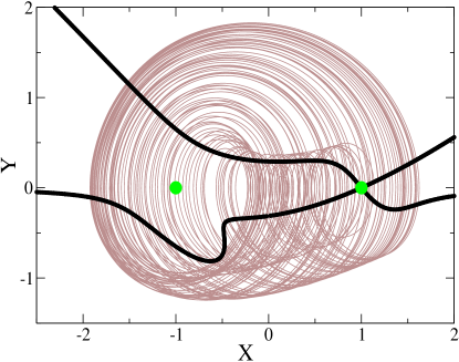
A stable limit cycle is produced for $R=0.15$. The fixed points are located at $x_{f_{1}}=-\sqrt{R}$ and $x_{f_{2}}=\sqrt{R}$. They have coordinates $(a,b,c)=(-B,-A,-2x_{f})$ in the catastrophe control parameter space shown in Fig. 7(c). Both fixed points reside in a region where they have a single pair of complex conjugate eigenvalues and two real eigenvalues ($\kappa_{1,2}=1$). The connecting curves and limit cycle for this case are shown in Fig. 10(a). The $n-2\kappa=2$ vortex core curves are observed to pass through each of the fixed points.

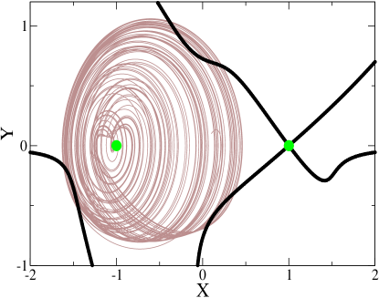
As $R$ is increased, the two fixed points scatter other along the $c$ axis. They retain the same value of $\kappa$ until the upper fixed point crosses the bifurcation boundary. The fixed point transition for $R=1$ is shown in Fig. 7(c). This value of $R$ generates the strange attractor shown in Fig. 10(b). The fixed points are located at $x_{f_{1}}=-1$ and $x_{f_{2}}=1$ with $\kappa_{1}=2$ and $\kappa_{2}=1$. The different $\kappa$ values plays an important role in the structure of strange attractor. Specifically, an asymmetry is created because $n-2\kappa_{2}=0$ connecting curves pass through $x_{f_{1}}$ and $n-2\kappa_{1}=2$ connecting curves pass through $x_{f_{2}}$.

Swirling flow generated near $x_{f_{2}}$ is transported along these two core curves towards $x_{f_{1}}$. The process creates a funnel in the center of the strange attractor. As the flow approaches the neighborhood of $x_{f_{1}}$, it is pushed back towards $x_{f_{2}}$ and the process is repeated. The two vortex core curves that connect to $x_{f_{2}}$ pass through the funnel of the strange attractor, but diverge to wrap around the hypervortex near $x_{f_{1}}$ since they are unable to attach to it.

Figure 9: Bifurcation diagram created using a single Poincaré surface of section along the X-axis (Y=0) for Eq. (9) with $G_{1}(x;R)=x^{2}-R$. A period doubling route to chaos is observed. Parameter values: $(A,B,C)=(-3.2,-2.335,-1)$.

Figure 10(c) shows an example of a strange attractor that forms in the hypervortex region around $x_{f_{1}}$ for a different set of control parameters $(A,B,C,R)=(-1.3,-2.6,-1.7,1)$. The vortex core curves in this case have less influence on the structure of the strange attractor.

(a) $(A,B,C,R)=(-3.2,-2.335,-1,0.15)$

(b) $(A,B,C,R)=(-3.2,-2.335,-1,1)$

(c) $(A,B,C,R):=(-1.3,-2.6,-1.7,1)$

Figure 10: $X-Y$ projection of the connecting curves, fixed points and phase space trajectories from Eq. (9) with $G_{1}(x;R)=x^{2}-R$. (a) Both fixed points have index $\kappa=1$. The phase space dynamics near the fixed points are described by a stable limit cycle. (b-c) Asymmetries in the vortex indices result in a fixed point with $\kappa=2$ (left) and one with $\kappa=1$ (right). The structure of the strange attractors is strongly influenced by the resulting vortices and hypervortices.

V.3 $m=3$

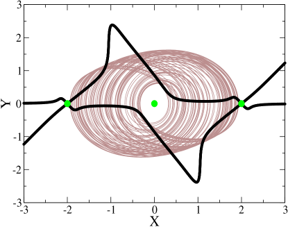
For $m=3$ we use $G_{1}(x;R)=x^{3}-Rx$ with control parameter values $(A,B,C,R)=(-3,-3.2,-1.43,4)$. The coordinates of the fixed points in the catastrophe control parameter space are given by $(a,b,c)=(-B,-A,-G_{1}^{\prime}(x_{f};R))$. Since $a>0$, the bifurcation surface splits the control parameter space into two regions. The symmetric fixed points share a single coordinate located in the region that produces a single pair of complex conjugate eigenvalues ($\kappa=1$) and two real eigenvalues. The fixed point at the origin is located in the region that produces two pairs of complex conjugate eigenvalues ($\kappa=2$). It is located in the hypervortex near the origin that plays an important role in the structure of the strange attractor shown in Fig. 11. The vortex core curves pass through the outer fixed points but are unable to enter the hypervortex that produces a hole in the center of the attractor.

Figure 11: X-Y projection of the strange attractor generated by Eq. (9) with $G_{1}(x;R)=x^{3}-Rx$. The hypervortex around the origin creates a hole in the attractor and forces the vortex core curves to wrap around it. Parameter values: $(A,B,C,R)=(-3,-3.2,-1.43,4)$

VI Five Dimensions

In this section we set $G_{2}(y,z,u,w;A,B,C,D)=Ay+Bz+Cu+Dw^{3}$ in order to study five-dimensional differential dynamical systems that take the form

$$\begin{array}[]{l}\dot{x}=y\\ \dot{y}=z\\ \dot{z}=u\\ \dot{u}=w\\ \dot{w}=G_{1}(x;R)+Ay+Bz+Cu+Dw^{3};\end{array}$$ (13)

The characteristic polynomial is

$$\begin{split}{\rm det}(J-\lambda I_{5}))=A_{5}(\lambda)=\\ \lambda^{5}-C\lambda^{3}-B\lambda^{2}-A\lambda-G_{1}^{\prime}(x_{f};R)\end{split}$$ (14)

where the substitution $(a,b,c,d)=(-C,-B,-A,-G_{1}^{\prime}(x_{f};R))$ creates the canonical unfolding of the next catastrophe in the series of cuspoids $A_{5}$. Here again the control parameter space is divided into three disjoint open regions that describe fixed points with zero, one, or two pairs of complex conjugate eigenvalues and a complementary number of real eigenvalues. The open regions are connected and simply connected and can be studied as in the case of $A_{4}(\lambda)$. We use $G_{1}(x_{1};R)=x^{2}-R$ in this section.

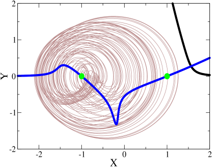
Parameters $(A,B,C,D,R)=(-1.8,-3.8,-3.1,-1,1)$ generate the strange attractor shown in Fig. 12. Both fixed points have two pairs of complex conjugate eigenvalues ($\kappa=2$) and $n-2\kappa=1$ hypervortex core curves connected to them. A vortex core curve ($\kappa=1$) is also observed to form away from the attractor.

Parameters $(A,B,C,D,R)=(-0.7,-7.0,-2.5,-1,1)$ generate the strange attractor shown in Fig. 13. The fixed point indices $\kappa$ of the two fixed points differ. A single hypervortex core curve runs through the fixed point $x_{f_{1}}$ with ($\kappa=2$) while $n-2\kappa=3$ vortex core curves run through the fixed point $x_{f_{2}}$ with ($\kappa=1$).

Figure 12: X-Y projection of the strange attractor generated by Eq. (5) using $G_{1}(x_{1};R)=x^{2}-R$. A hypervortex core curve ($\kappa=2$) connects the two fixed points. Parameter values: $(A,B,C,D,R)=(-1.8,-3.8,-3.1,-1,1)$.

Figure 13: X-Y projection of the attractor generated by Eq. (5) using $G_{1}(x_{1};R)=x^{2}-R$. A single hypervortex core curve ($\kappa=2$) runs through the fixed point on the left. After a change in stability, three vortex core curves run through the fixed point on the right with $\kappa=1$. Parameter values: $(A,B,C,D,R)=(-0.7,-7.0,-2.5,-1.0,1.0)$

VII Conclusions

The present work was motivated by an attempt to determine how invariant sets of greater dimension than fixed points can be used to determine the structure of flows that result from integrating sets of nonlinear ordinary different equations. These sets, which have been called core curves, obey the eigenvalue-like equation $J{\bf f}=\lambda{\bf f}$ and have previously been used in studies of three-dimensional flows. In extending these results to higher dimensions, we have focused on a special class of dynamical systems — differential dynamical systems as defined in Eq. (1), which have the same form in all dimensions $n\geq 3$. Only the driving function $F(x_{1},\dots,x_{n};c)$ varies from system to system.

Since all fixed points occur on the $x_{1}$ axis, it was convenient to write the driving function as a sum of two functions, $G_{1}(x_{1};c_{1})$ depending only on the coordinate $x_{1}$ and a set of control parameters $c_{1}$, and another function $G_{2}(x_{2},\dots,x_{n};c_{2})$ depending on complementary variables. The locations of the fixed points can be put into canonical form by expressing $G_{1}$ in terms of a cuspoid catastrophe $A_{m}^{\prime}(x_{1};c_{1})=x^{m}+ax^{m-2}+\dots$, where $m$ is the maximum number of fixed points that occurs under control parameter variation. The stability at a fixed point is determined by the first derivatives $\partial G_{2}/\partial x_{i}$, evaluated at $x_{i}=0$, $i=2,\dots,n$, and $\partial G_{1}/\partial x_{1}$. That is, the stability is governed by the linear terms in $G_{2}(x_{2},\dots,x_{n};c_{2})$ and the slope of $G_{1}$. Variations in the stability of the fixed points is most conveniently studied by identifying the linearization of $G_{2}$ with another cuspoid catastrophe $A_{n}^{\prime}(x_{1};c_{1})=x^{n}+ax^{n-2}+\dots$, where $n$ is the dimension of the dynamical system. There is a weak coupling between these two catastrophes given by the term $G_{1}^{\prime}(x_{1};c_{1})$, which appears as one of the unfolding parameters for the function $G_{2}$. The slope alternates along the $x_{1}$ axis from fixed point to fixed point.

Table 1: Summary of the equations studied.

$$\begin{array}[]{cccccc}{\rm Eq.}&n&\#{\rm F.P.}&G_{1}(x)&G_{2}&{\rm Fig.}\\ \hline\cr\ref{eq:3dode}&3&2&x^{2}-R&Ay+By^{2}z&\ref{fig:SaddleNode},\ref{fig:reconnect},\ref{fig:VortStrain}\\ \ref{eq:3dode}&3&3&x^{3}-Rx&Ay+By^{2}z&\ref{fig:3d3fpXY}\\ \ref{eq:4dode}&4&1&Rx&Ay+Bz+Cu^{3}&\ref{fig:4d1fp}\\ \ref{eq:4dode}&4&2&x^{2}-R&Ay+Bz+Cu^{3}&\ref{fig:4d2fp}\\ \ref{eq:4dode}&4&3&x^{3}-Rx&Ay+Bz+Cu^{3}&\ref{fig:4d3fp}\\ \ref{eq:5dode}&5&2&x^{2}-R&Ay+Bz+Cu+Dw^{3}&\ref{fig:5d2fp2-2},\ref{fig:5d2fp2-1}\\ \end{array}$$

At a fixed point the core curves are tangent to the eigenvectors of $J$ with real eigenvalues. There are $n-2\kappa$ real eigenvalues, where $\kappa$ is the number of complex conjugate pairs of eigenvalues. If $n-2\kappa\geq 1$ and $\kappa\geq 1$ then a core curve emanating from the fixed point may pass through the “center” of a strange attractor and act to organize the flow around it. If $\kappa=1$ the curve is called a vortex core curve and if $\kappa>1$ it is called a hypervortex core curve. If $\kappa=0$ then only strain curves ($n$ of them) originate at the fixed point. If $n-2\kappa=0$ then the fixed point is disconnected from the network of curves satisfying the defining eigenvalue-like equation.

The eigenvalues of the jacobian at a fixed point vary as the control parameters vary. If a real (complex conjugate) pair becomes degenerate and scatters to become a complex conjugate (real) pair, then two distinct core curves gradually approach degeneracy and then detach from (attach to) the fixed point.

The eigenvalues of the jacobian also vary along core curves. Changes in stability and/or the number of real and complex conjugate pairs are closely involved in rearrangements or recombinations of the core curves.

For differentiable dynamical systems the eigenvalue equation defining the core curve can be projected to a pair of constraints acting in a three-dimensional space. This pair of constraints is given in Eq. (15). Core curves are not heteroclinic connections in the dynamical system. Rather, they satisfy a closely related set of nonlinear equations that are effectively nonautonomous. This dynamical system is given in Eq. (16).

These ideas have been illustrated for dynamical systems with $n=3,m=2,3$, $n=4,m=1,2,3$ and $n=5,m=2$. Table 1 summarizes the cases presented, the dynamical system equations studied, and the figures that illustrate the results. Supplementary material from this work can be found online supplementary .

VIII Acknowledgements

We thank Fernando Mut for useful discussion.

IX Appendix 1

Core curves for differential dynamical systems obey the condition $x_{i+1}=\lambda x_{i}$, so that $x_{k}=\lambda^{k-2}x_{2}$ for $k=3,\dots,n$. As a result there are three independent variables $\lambda,x_{1},x_{2}$ and two constraints:

$$\left[\begin{array}[]{cc}0&1\\ \sum_{j=1}^{n-1}\lambda^{j-1}F_{j}&F_{n}\end{array}\right]\left[\begin{array}[]{c}x_{2}\\ F\end{array}\right]=\lambda\left[\begin{array}[]{c}\lambda^{n-2}x_{2}\\ F\end{array}\right]$$ (15)

The functions that appear in this collapsed constraint equation are obtained by replacing $x_{k}\rightarrow\lambda^{k-2}x_{2}$. The general form for the vortex core curve is independent of the dimension $n$ of the differential dynamical system and is described by a curve in the space $R^{3}$ with coordinates $(\lambda,x_{1},x_{2})$.

A dynamical equation that core curves satisfy has the form

$$\left(\frac{\partial^{2}f_{i}}{\partial x_{j}\partial x_{k}}f_{j}+\frac{\partial f_{i}}{\partial x_{j}}\frac{\partial f_{j}}{\partial x_{k}}-\lambda\frac{\partial f_{i}}{\partial x_{k}}\right)\frac{dx_{k}}{d\lambda}=f_{i}$$ (16)

References

- (1) R. Gilmore, J.-M. Ginoux, Timothy Jones, C. Letellier, and U. S. Freitas, Connecting curves for dynamical systems, J. Phys. A, 43, 255101, (2010).
- (2) M. Roth and R. Peikert, A higher-order method for finding vortex core lines, Proceedings IEEE of the conference on Visualization’98, 143-150 (1998).
- (3) R. Peikert and M. Roth, The “parallel vectors” operator: a vector field visualization primitive, Proceedings IEEE of the conference on Visualization ’99, 263-270 (1999).
- (4) V. I. Arnold, On matrices depending on parameters, Russian Math Surveys 26, 29-43 (1971).
- (5) R. Gilmore, Catastrophe Theory for Scientists and Engineers, New York: Wiley, 1981.
- (6) R. Thom, Stabilité Structurelle et Morphogénèse, NY: Benjamin, 1971.
- (7) E. C. Zeeman, Catastrophe Theory: Selected Papers 1971-1976, Berlin-New York: Springer-Verlag, 1976.
- (8) T. Poston and I. N. Stewart, Catastrophe Theory, New York: Dover, 1978.
- (9) https://sites.google.com/site/gr9gbyrne/supplementary-material