Finite Volume Modeling of Poroelastic-Fluid Wave Propagation with Mapped Grids

Abstract

In this work we develop a high-resolution mapped-grid finite volume method code to model wave propagation in two dimensions in systems of multiple orthotropic poroelastic media and/or fluids, with curved interfaces between different media. We use a unified formulation to simplify modeling of the various interface conditions — open pores, imperfect hydraulic contact, or sealed pores — that may exist between such media. Our numerical code is based on the clawpack framework, but in order to obtain correct results at a material interface we use a modified transverse Riemann solution scheme, and at such interfaces are forced to drop the second-order correction term typical of high-resolution finite volume methods. We verify our code against analytical solutions for reflection and transmission of waves at a material interface, and for scattering of an acoustic wave train around an isotropic poroelastic cylinder. For reflection and transmission at a flat interface, we achieve second-order convergence in the 1-norm, and first-order in the max-norm; for the cylindrical scatterer, the highly distorted grid mapping degrades performance but we still achieve convergence at a reduced rate. We also simulate an acoustic pulse striking a simplified model of a human femur bone, as an example of the capabilities of the code. To aid in reproducibility, at the web site http://dx.doi.org/10.6084/m9.figshare.701483 we provide all of the code used to generate the results here.

1 Introduction

Poroelasticity theory was developed by Maurice A. Biot to model the mechanics of a fluid-saturated porous medium. It models the medium in a homogenized fashion, with solid portion treated with linear elasticity, and the fluid with linearized compressible fluid dynamics combined with Darcy’s law to relate its pressure gradient to its flow rate. Biot’s work is summarized in his 1956 and 1962 papers [3, 4, 5], and Carcione also provides an excellent discussion of poroelasticity in chapter 7 of his book [9]. While it was originally developed to model fluid-saturated rock and soil, Biot theory has also found applications in modeling of in vivo bone [13, 14, 20] and underwater acoustics with a porous sea floor [7, 21, 22].

Biot theory predicts three different families of propagating waves within a poroelastic medium. In order of decreasing speed, these are: fast P waves, where the fluid and solid parts of the medium move roughly parallel to the propagation direction — exactly parallel for an isotropic medium — and are typically in phase with each other; S waves, where the motion of the medium is transverse to the propagation direction; and slow P waves, where the motion is again roughly parallel to the wavevector but the fluid and solid typically move 180 degrees out of phase, so that the fluid is leaving a region as the solid contracts, and vice versa. Because Biot theory includes viscous drag between the walls of the pore structure and the fluid, all three families of waves dissipate as they propagate through the medium; the slow P wave typically involves much more relative motion between the solid and fluid than the other two waves, so it is much more strongly damped.

Researchers have used a variety of numerical methods to model poroelasticity. Carcione, Morency, and Santos provide a detailed chronicle [10], and we provide a brief review in the introduction to our previous paper [33]. In this paper we wish to particularly draw attention to the work of Chiavassa and Lombard [11, 12], who model problems very similar to the ones we analyze. They use a fourth-order finite difference method to solve a first-order velocity-stress form of Biot’s equations, coupled with operator splitting to handle the viscous dissipation term, and employ an immersed interface approach at the boundary between the fluid and solid parts of the domain.

This paper extends our previous work in finite volume modeling of a first-order velocity-stress formulation of Biot poroelasticity theory [33] to include non-rectilinear mapped grids and bounded interfaces between poroelastic media and fluids. Both of these capabilities are important for applications such as ocean bottom acoustics, where the bottom bathymetry may be uneven and waves propagate from the water into the ocean floor and back again, and applications to wave propagation in bone, since bones are rarely rectangular in shape and can benefit from a fitted grid, and wave propagation between bone and the surrounding fluid or soft tissue is again important. We also implement explicit interface conditions between distinct poroelastic media, such as those proposed by Deresiewicz and Skalak [17]. We continue to employ the clawpack finite volume method package [40], which substantially reduces the programming time and effort required for this work; clawpack also offers built-in operator splitting, as well as adaptive mesh refinement if desired [2]. We develop a technique to solve the Riemann problem efficiently for grid interfaces oriented at arbitrary angles in anisotropic poroelastic media, as well as modifications to the classical high-resolution finite volume method that are necessary to obtain qualitatively correct solutions to problems with fluid-poroelastic interfaces. We then proceed to verify our code against known analytical solutions involving interfaces in both rectilinear and curved geometries, and analyze a sample biological problem of an acoustic wave striking a simplfied model of a human femur bone.

2 Governing PDEs and interface conditions

A poroelastic medium consists of a porous solid skeleton or matrix, saturated with a fluid. We use essentially the same first-order formulation of Biot poroelasticity theory in two dimensions as in our previous work [33], with the order of the variables in the state vector permuted in order to emphasize the block structure of the system. The state variables at a point are the total stress tensor $\tau$ (the combined stress from the solid skeleton and the fluid pressure), the fluid pressure $p$, the solid velocity $\mathbf{v}$, and the fluid volumetric flow velocity $\mathbf{q}$ relative to the solid, which is equal to the fluid velocity relative to the solid divided by the porosity $\phi$. This section gives only a quick summary of the system of PDEs and ancillary functionals; readers desiring more detail are encouraged to refer to [33], Biot’s papers of 1956 [3, 4] and 1962 [5], or Carcione’s book [9].

In addition to purely poroelastic systems, we also model systems composed of a combination of poroelastic and fluid media. We model the fluid parts of these systems using linear acoustics; this subject is well-understood, so we discuss it only briefly here. Of more interest are the conditions that must be satisifed at the interfaces between different media, both between a fluid and a poroelastic medium and between two distinct poroelastic media. This section covers these interface conditions in their root form at the PDE level, though we defer discussion of their implementation in the numerical code to Section 3.

2.1 Poroelasticity system

First, define the state vector $\mathbf{Q}$ at a point in a poroelastic medium as

$$\mbox{$\mathbf{Q}$}=\begin{pmatrix}p&\tau_{xx}&\tau_{zz}&\tau_{xz}&v_{x}&v_{z}&q_{x}&q_{z}\end{pmatrix}^{T}.$$ (1)

Here $p$ is the pressure of the fluid in the pores, $\tau$ is the total stress tensor, $\mathbf{v}$ is the velocity of the solid component of the medium, and $\mathbf{q}$ is the flow rate of the fluid relative to the solid. The $x$ and $z$ axes are the global axes in which the problem is defined. Note that this state vector contains the same quantities as the one defined in [33], but arranged in a different order.

For this work, we deal with orthotropic media: media that possess a set of three perpendicular planes of symmetry, so that in the axes defined by these planes, extensional and shear deformation are decoupled. We call these the principal axes of the medium, and denote them by the numbers $1$, $2$, and $3$ to distinguish them from the $x$ and $z$ axes. We also make the assumption that the our poroelastic media are transversely isotropic — specifically, isotropic in the $1$-$2$ plane — and that axes $1$ and $3$ lie in the $x$-$z$ plane. This type of anisotropy is common in engineering composites [19] and in some biological materials [15], as well as being present in certain types of stone. However, this assumption is not a fundamental requirement of our work — it simplifies the system matrices, but it would be straightforward to extend our formulation to general anisotropic materials.

Following [33], in a homogeneous medium with no sources the equations of Biot poroelasticity theory at low frequency can be expressed as an $8\times 8$ first-order linear system of PDEs,

$$\partial_{t}\mbox{$\mathbf{Q}$}+\mbox{$\mathbf{A}$}\partial_{x}\mbox{$\mathbf{Q}$}+\mbox{$\mathbf{B}$}\partial_{z}\mbox{$\mathbf{Q}$}=\mbox{$\mathbf{D}$}\mbox{$\mathbf{Q}$}.$$ (2)

We also frequently work with the homogeneous form of this system,

$$\partial_{t}\mbox{$\mathbf{Q}$}+\mbox{$\mathbf{A}$}\partial_{x}\mbox{$\mathbf{Q}$}+\mbox{$\mathbf{B}$}\partial_{z}\mbox{$\mathbf{Q}$}=0.$$ (3)

In particular, the homogeneous form is the form of the system we use when solving the Riemann problem for our high-resolution finite volume scheme.

With the state vector in (1), the coefficient matrices can be written in block form,

$$\mbox{$\mathbf{A}$}=\begin{pmatrix}0_{4\times 4}&\mbox{$\mathbf{A}$}_{sv}\\ \mbox{$\mathbf{A}$}_{vs}&0_{4\times 4}\end{pmatrix},\quad\mbox{$\mathbf{B}$}=\begin{pmatrix}0_{4\times 4}&\mbox{$\mathbf{B}$}_{sv}\\ \mbox{$\mathbf{B}$}_{vs}&0_{4\times 4}\end{pmatrix},\quad\mbox{$\mathbf{D}$}=\begin{pmatrix}0_{4\times 4}&0_{4\times 4}\\ 0_{4\times 4}&\mbox{$\mathbf{D}$}_{v}\end{pmatrix}.$$ (4)

If the computational $x$-$z$ axes coincide with the principal $1$-$3$ axes of the material, the blocks in (4) are

$$\mbox{$\mathbf{A}$}_{sv} =\begin{pmatrix}\alpha_{1}M&0&M&0\\ -c_{11}^{u}&0&-\alpha_{1}M&0\\ -c_{13}^{u}&0&-\alpha_{3}M&0\\ 0&-c_{55}^{u}&0&0\end{pmatrix} \mbox{$\mathbf{A}$}_{vs} =\begin{pmatrix}-\frac{\rho_{f}}{\Delta_{1}}&-\frac{m_{1}}{\Delta_{1}}&0&0\\ 0&0&0&-\frac{m_{3}}{\Delta_{3}}\\ \frac{\rho}{\Delta_{1}}&\frac{\rho_{f}}{\Delta_{1}}&0&0\\ 0&0&0&\frac{\rho_{f}}{\Delta_{3}}\end{pmatrix}$$ (5)

$$\mbox{$\mathbf{B}$}_{sv} =\begin{pmatrix}0&\alpha_{3}M&0&M\\ 0&-c_{13}^{u}&0&-\alpha_{1}M\\ 0&-c_{33}^{u}&0&-\alpha_{3}M\\ -c_{55}^{u}&0&0&0\end{pmatrix} \mbox{$\mathbf{B}$}_{vs} =\begin{pmatrix}0&0&0&-\frac{m_{1}}{\Delta_{1}}\\ -\frac{\rho_{f}}{\Delta_{3}}&0&-\frac{m_{3}}{\Delta_{3}}&0\\ 0&0&0&\frac{\rho_{f}}{\Delta_{1}}\\ \frac{\rho}{\Delta_{3}}&0&\frac{\rho_{f}}{\Delta_{3}}&0\end{pmatrix}$$ (6)

$$\mbox{$\mathbf{D}$}_{v} =\begin{pmatrix}0&0&\frac{\rho_{f}\eta}{\Delta_{1}\kappa_{1}}&0\\ 0&0&0&\frac{\rho_{f}\eta}{\Delta_{3}\kappa_{3}}\\ 0&0&-\frac{\rho\eta}{\Delta_{1}\kappa_{1}}&0\\ 0&0&0&-\frac{\rho\eta}{\Delta_{3}\kappa_{3}}\end{pmatrix}.$$ (7)

Here the subscripts $s$ and $v$ denote the stress variables ($p$ and $\tau$) and velocity variables ($\mathbf{v}$ and $\mathbf{q}$), respectively. The entries in these matrices are determined from the physical properties in Table 1; the parameters $c_{ij}^{u}$ are the undrained elastic stiffness constants, which are determined from the drained stiffness constants $c_{ij}$, the effective stress coefficients $\alpha_{i}$, and the bulk compressibility parameter $M$. Ordering the variables to highlight this block structure emphasizes the underlying physics — gradients of stress produce changes in velocity, and gradients of velocity produce changes in stress — but it also proves useful mathematically. If the $x$-$z$ axes do not coincide with the material principal axes, we can obtain appropriate $\mathbf{A}$, $\mathbf{B}$, and $\mathbf{D}$ matrices by transforming the state variables $\mathbf{Q}$ into the new axes and applying the chain rule of partial differentiation. We refer the reader to our previous paper [33], or to Carcione’s book [9], for full explanation of the parameters in these matrices.

2.2 Energy density for poroelasticity

In [33] we derived the energy density associated with a state vector $\mathbf{Q}$ as

$$\mathcal{E}=\frac{1}{2}\mbox{$\mathbf{Q}$}^{T}\mbox{$\mathbf{E}$}\mbox{$\mathbf{Q}$}.$$ (8)

The Hessian of the energy density $\mathbf{E}$ remains symmetric after the elements of $\mathbf{Q}$ are permuted to the order used here; with the new ordering, $\mathbf{E}$ takes the block diagonal form

$$\mbox{$\mathbf{E}$}=\begin{pmatrix}\mbox{$\mathbf{E}$}_{s}&0_{4\times 4}\\ 0_{4\times 4}&\mbox{$\mathbf{E}$}_{v}\end{pmatrix},$$ (9)

where in the principal material axes the diagonal blocks of $\mathbf{E}$ are

$$\mbox{$\mathbf{E}$}_{s} =\begin{pmatrix}\frac{1}{M}+\frac{\alpha_{1}^{2}c_{33}+\alpha_{3}^{2}c_{11}-2\alpha_{1}\alpha_{3}c_{13}}{c_{11}c_{33}-\left(c_{13}\right)^{2}}&\frac{\alpha_{1}c_{33}-\alpha_{3}c_{13}}{c_{11}c_{33}-\left(c_{13}\right)^{2}}&\frac{\alpha_{3}c_{11}-\alpha_{1}c_{13}}{c_{11}c_{33}-\left(c_{13}\right)^{2}}&0\\ \frac{\alpha_{1}c_{33}-\alpha_{3}c_{13}}{c_{11}c_{33}-\left(c_{13}\right)^{2}}&\frac{c_{33}}{c_{11}c_{33}-\left(c_{13}\right)^{2}}&-\frac{c_{13}}{c_{11}c_{33}-\left(c_{13}\right)^{2}}&0\\ \frac{\alpha_{3}c_{11}-\alpha_{1}c_{13}}{c_{11}c_{33}-\left(c_{13}\right)^{2}}&-\frac{c_{13}}{c_{11}c_{33}-\left(c_{13}\right)^{2}}&\frac{c_{11}}{c_{11}c_{33}-\left(c_{13}\right)^{2}}&0\\ 0&0&0&\frac{1}{c_{55}}\\ \end{pmatrix}$$ (10)

$$\mbox{$\mathbf{E}$}_{v} =\begin{pmatrix}\rho&0&\rho_{f}&0\\ 0&\rho&0&\rho_{f}\\ \rho_{f}&0&m_{1}&0\\ 0&\rho_{f}&0&m_{3}\end{pmatrix}.$$

Note that the individual blocks $\mbox{$\mathbf{E}$}_{s}$ and $\mbox{$\mathbf{E}$}_{v}$ are themselves symmetric positive-definite matrices. The parameters $c_{ij}$ are the drained elastic stiffness constants.

This energy density allows us to define in a natural way a norm for the state vector $\mathbf{Q}$ that bypasses problems with relative scaling of its components when they are expressed in typical unit systems. We define the energy inner product of two state vectors $\mbox{$\mathbf{Q}$}_{1}$ and $\mbox{$\mathbf{Q}$}_{2}$ as

$$\langle\mbox{$\mathbf{Q}$}_{1},\mbox{$\mathbf{Q}$}_{2}\rangle_{E}:=\mbox{$\mathbf{Q}$}_{2}^{H}\mbox{$\mathbf{E}$}\mbox{$\mathbf{Q}$}_{1}.$$ (11)

(We use the Hermitian conjugate-transpose here to ensure that this remains an inner product if it is extended to complex vectors.) From this inner product, we define the induced energy norm,

$$\|\mbox{$\mathbf{Q}$}\|_{E}:=\sqrt{\langle\mbox{$\mathbf{Q}$},\mbox{$\mathbf{Q}$}\rangle_{E}}.$$ (12)

As discussed in [33], the matrix $\mathbf{E}$ allows us to show several useful properties of the system, including the $\mathbf{E}$-orthogonality of the eigenvectors of $\mathbf{A}$, $\mathbf{B}$, or any linear combination of them, and the fact that the energy density $\mathcal{E}$ is a strictly convex entropy function of the system. The $\mathbf{E}$-orthogonality of the eigenvectors also allows an easy proof that the system is hyperbolic.

2.3 Linear acoustics

The partial differential equations governing linear acoustics are well-known, and we will not re-derive them here. We will, however, state how they are incorporated into the same framework as poroelasticity.

We use the same form of first-order linear system as (2) to model acoustic wave propagation in a fluid, with the same state vector; however, in a fluid we define the variables $\tau$ and $\mathbf{v}$ to be identically zero. We use $p$ for the fluid pressure and $\mathbf{q}$ for its velocity. (In fact the total stress tensor in the fluid is $-p\mathbf{I}$, but it is more convenient to use the single pressure variable and ignore $\tau$ in the fluid.) The appropriate coefficient matrices have the same block form as for poroelasticity, with blocks given by

$$\mbox{$\mathbf{A}$}_{sv} =\begin{pmatrix}0&0&K_{f}&0\\ 0&0&0&0\\ 0&0&0&0\\ 0&0&0&0\end{pmatrix} \mbox{$\mathbf{A}$}_{vs} =\begin{pmatrix}0&0&0&0\\ 0&0&0&0\\ \frac{1}{\rho_{f}}&0&0&0\\ 0&0&0&0\end{pmatrix}$$ (13)

$$\mbox{$\mathbf{B}$}_{sv} =\begin{pmatrix}0&0&0&K_{f}\\ 0&0&0&0\\ 0&0&0&0\\ 0&0&0&0\end{pmatrix} \mbox{$\mathbf{B}$}_{vs} =\begin{pmatrix}0&0&0&0\\ 0&0&0&0\\ 0&0&0&0\\ \frac{1}{\rho_{f}}&0&0&0\end{pmatrix}.$$ (14)

The dissipation matrix $\mathbf{D}$ is identically zero for a fluid.

Similarly to a poroelastic medium, we can also write a matrix $\mathbf{E}$ such that the energy density in the fluid is $\mathcal{E}=\frac{1}{2}\mbox{$\mathbf{Q}$}^{T}\mbox{$\mathbf{E}$}\mbox{$\mathbf{Q}$}$. This $\mathbf{E}$ matrix has the same block structure as for poroelasticity; its blocks are

$$\mbox{$\mathbf{E}$}_{s} =\begin{pmatrix}\frac{1}{K_{f}}&0&0&0\\ 0&0&0&0\\ 0&0&0&0\\ 0&0&0&0\end{pmatrix}, \mbox{$\mathbf{E}$}_{v} =\begin{pmatrix}0&0&0&0\\ 0&0&0&0\\ 0&0&\rho_{f}&0\\ 0&0&0&\rho_{f}\end{pmatrix}.$$ (15)

Note that the $\mathbf{E}$ defined this way is only positive-semidefinite, not positive-definite as for poroelasticity. However, the null space of $\mathbf{E}$ consists only of the variables that are defined to be identically zero in the fluid, so it is essentially positive-definite, and it is still sensible to use it to define an energy inner product and norm in the fluid.

2.4 Interface conditions

Nontrivial conditions relating the state variables on either side of an interface between distinct poroelastic materials have been proposed by a number of authors. These include Deresiewicz and Skalak [17], who proposed an imperfect hydraulic contact condition relating the pressure difference across the interface to the normal fluid flow rate, and Sharma [38], who formulated a loose contact condition modeling lubricated slippage between the two sides. For this work, we use Deresiewicz and Skalak’s imperfect hydraulic contact condition; Deresiewicz and Skalak showed that this condition is sufficient to give a unique solution to Biot’s equations in a discontinuous medium, and Gurevich and Schoenberg [24] examined how such a condition could arise asymptotically from a smoothly varying medium as the region over which the material properties vary is shrunk to zero thickness.

The imperfect hydraulic contact condition can be written in the form

$$\mbox{\boldmath$\tau$}_{l}\cdot\mathbf{n} =\mbox{\boldmath$\tau$}_{r}\cdot\mathbf{n}$$ (16)

$$\mathbf{v}_{l} =\mathbf{v}_{r}$$

$$\mathbf{q}_{l}\cdot\mathbf{n} =\mathbf{q}_{r}\cdot\mathbf{n}$$

$$p_{l}-p_{r} =\frac{1}{\mathcal{K}}\widehat{\mathbf{q}\cdot\mathbf{n}}.$$

Here the subscripts $l$ and $r$ represent the left and right sides of the interface, chosen arbitrarily, and $\mathbf{n}$ is the unit normal to the interface, pointing from left to right. These equations have direct physical significance: the first is a statement of the continuity of traction across the interface, the second states that the materials stay connected to each other, the third requires that all fluid entering the interface should exit the other side, and the fourth relates the fluid flow rate across the interface to the pressure difference forcing it across. The parameter $\mathcal{K}$ is a measure of the ability of the interface to conduct fluid, and ranges from zero, representing a completely impermeable interface, to $+\infty$, representing no impedance to fluid flow. The quantity $\widehat{\mathbf{q}\cdot\mathbf{n}}$ is the volume flow rate of fluid across the interface, which is equal to both $\mathbf{q}_{l}\cdot\mathbf{n}$ and $\mathbf{q}_{r}\cdot\mathbf{n}$ according to the third equation of (16). We will revisit this ambiguity when we discuss the implementation of this interface condition. Our previous work [33], which simply used the wave structure of the system without any explicit interface condition, was equivalent to this condition with $\mathcal{K}=+\infty$; Gurevich and Schoenberg [24] showed that this is the most natural interface condition in the context of Biot’s equations as a PDE system, and we continue to use the same approach where no discontinuities in the medium are present.

Since both $\mathcal{K}=0$ and $\mathcal{K}=+\infty$ are common and important cases, and since infinite values are inconvenient in numerical computations, we reparameterize the fourth equation of (16). Noting that $1/\mathcal{K}$ has the same units as acoustic impedance, we define

$$\frac{1}{\mathcal{K}}=:Z_{f}\frac{1-\eta_{d}}{\eta_{d}},$$ (17)

where $Z_{f}$ is the impedance of the pore fluid in the left medium and $\eta_{d}\in[0,1]$ is a new nondimensional parameter we term the interface discharge efficiency. Setting $\mathcal{K}=+\infty$ now corresponds to setting $\eta_{d}=1$, and $\mathcal{K}=0$ corresponds to $\eta_{d}=0$. Substituting this into the fourth equation of (16) and multiplying through by $\eta_{d}$, we obtain

$$\mbox{\boldmath$\tau$}_{l}\cdot\mathbf{n} =\mbox{\boldmath$\tau$}_{r}\cdot\mathbf{n}$$ (18)

$$\mathbf{v}_{l} =\mathbf{v}_{r}$$

$$\mathbf{q}_{l}\cdot\mathbf{n} =\mathbf{q}_{r}\cdot\mathbf{n}$$

$$\eta_{d}(p_{l}-p_{r}) =Z_{f}(1-\eta_{d})\widehat{\mathbf{q}\cdot\mathbf{n}},$$

which presents no special difficulty for any value of $\eta_{d}$, including 0 and 1. This is the form of the interface condition that we use in our numerical computations.

Between a poroelastic medium and a fluid, we use a similar condition, which we write as

$$\mathbf{q}_{f}\cdot\mathbf{n} =(\mathbf{v}_{p}+\mathbf{q}_{p})\cdot\mathbf{n}$$ (19)

$$-p_{f}\mathbf{n} =\mbox{\boldmath$\tau$}_{p}\cdot\mathbf{n}$$

$$p_{p}-p_{f} =\frac{1}{\mathcal{K}}\mathbf{q}_{p}\cdot\mathbf{n}.$$

Here, the subscript $f$ indicates quantities in the fluid, while $p$ indicates quantities in the poroelastic medium. We use $\mathbf{q}_{f}$ for the fluid velocity, and the unit interface normal $\mathbf{n}$ points from the poroelastic medium into the fluid. The meanings of the equations are similar to before: the first states continuity of fluid flow, the second, continuity of traction, and the third relates fluid flow rate to pressure difference. The parameter $\mathcal{K}$ has the same meaning as before, though its value may be different. This condition models possibly imperfect hydraulic contact; it seems to have been first used at a poroelastic-fluid interface by Rosenbaum [37], and has since been employed by other authors [6, 18]. Chiavassa and Lombard [11] in particular use this method in their numerical work, and also demonstrate that the resulting coupled systems of PDEs on the fluid and poroelastic domains are well-posed. For easier implementation, we again replace $1/\mathcal{K}$ with $Z_{f}(1-\eta_{d})/\eta_{d}$, where $Z_{f}$ is the acoustic impedance of the fluid medium, obtaining the alternative form

$$\mathbf{q}_{f}\cdot\mathbf{n} =(\mathbf{v}_{p}+\mathbf{q}_{p})\cdot\mathbf{n}$$ (20)

$$-p_{f}\mathbf{n} =\mbox{\boldmath$\tau$}_{p}\cdot\mathbf{n}$$

$$\eta_{d}(p_{p}-p_{f}) =Z_{f}(1-\eta_{d})\mathbf{q}_{p}\cdot\mathbf{n}.$$

3 Finite volume methods for poroelastic-fluid systems on logically rectangular mapped grids

In order to be able to model geometries that do not lend themselves to the straight lines and 90 degree angles of a rectilinear grid, we use logically rectangular mapped grids. Compared to unstructured grids, mapped grids have the advantage of simpler data structures and less computational overhead, although creating the desired mapping function is not always trivial. They also combine well with finite volume methods, since the finite volume solution tends to maintain good quality even in the face of a mapping that severely distorts the grid. However, when modeling anisotropic poroelastic media, having to deal with cell interfaces that may be oriented in any arbitrary direction means that the simple compute-and-cache method used to solve the Riemann problem in our previous work no longer suffices. Section 3.2 discusses a Riemann solution process designed to function efficiently in this context, and to also incorporate interface conditions such as (18) and (20).

An additional difficulty we encounter is that at an interface between a poroelastic medium and a fluid, the classical formulation of a high-resolution finite volume method can be qualitatively incorrect — the classical transverse and second-order correction fluxes result in poroelastic variables such as skeleton stress and solid velocity being carried into the fluid, where they make no sense. We discuss this further in section 3.3, and are able to produce qualitatively correct solutions, though the best way to fully reformulate the method, including generalizations of the classical limiters and second-order correction fluxes, is still an open question.

In the remaining parts of this section, we briefly discuss the implementation of the source term in the poroelasticity system and the clawpack software framework in which we implement our numerical solution.

3.1 Mapped grids

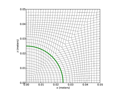
For a mapped grid approach, we start with a uniform rectangular grid in the computational coordinates, denoted $\xi_{1}$ and $\xi_{2}$. We then apply a mapping function $\mathbf{X}(\xi_{1},\xi_{2})$ to obtain the grid in physical coordinates $(x,z)$. This mapping function is typically chosen so that the grid boundaries or interior grid lines follow some feature of interest in the problem, although once the grid mapping is formulated, the actual cells are taken to be quadrilaterals with straight sides, whose vertices are obtained using the mapping function. Each grid cell $ij$ has an associated capacity $\kappa_{ij}$, which is the ratio of the area of the cell in physical coordinates to its area $\Delta\xi_{1}\,\Delta\xi_{2}$ in computational coordinates, and each cell interface has an associated unit normal vector $\mathbf{n}$ pointing in the positive grid direction. Figure 1 shows an example of a mapped grid. Finite volume methods on mapped grids are discussed in greater detail in Chapter 23 of [34].

Fig. 1: Example of a mapped grid, showing computational space at the left and physical space at the right.

3.2 Riemann problems on mapped grids

One of the most critical parts of any high-resolution finite volume code is the solution of the Riemann problem. Solving the Riemann problem for poroelasticity at first appears challenging due to the size and complexity of the hyperbolic part of the system (2). However, by taking advantage of the structure of the system, a straightforward and fairly efficient solution is possible.

3.2.1 Eigenvalues and eigenvectors

The first order of business in solving the Riemann problem is finding the eigenvectors of $\breve{\mbox{$\mathbf{A}$}}=n_{x}\mbox{$\mathbf{A}$}+n_{z}\mbox{$\mathbf{B}$}$ corresponding to the propagating waves, and the corresponding eigenvalues giving the wave speeds. For linear acoustics, this eigensystem is simple: the eigenvalues are $\pm\sqrt{K_{f}/\rho_{f}}$, and the eigenvectors may be easily verified as

$$\mathbf{r}_{\text{acoustic, left}} =\begin{pmatrix}-Z_{f}&0&0&0&0&0&n_{x}&n_{z}\end{pmatrix}^{T}$$ (left-going wave) (21)

$$\mathbf{r}_{\text{acoustic, right}} =\begin{pmatrix}Z_{f}&0&0&0&0&0&n_{x}&n_{z}\end{pmatrix}^{T} \text{(right-going wave)}.$$

For poroelasticity the eigensystem is substantially more complicated, but it is possible to exploit the block structure, symmetry, and simple null space of the poroelastic system to reduce the eigenproblem from an $8\times 8$ non-symmetric to a $3\times 3$ real symmetric one; see Appendix A for details. As a note on implementation, our code caches the eigensystems computed for each Riemann problem, and checks whether the next Riemann problem has the same input data to the eigensolves; if so, the previous eigensystem is re-used. This speeds up execution in the common special case of large sections of the domain that have straight grid lines and uniform composition.

3.2.2 Solution between identical materials

The solution of the Riemann problem for linear acoustics with identical media on either side of the interface is simple and well-known, and will not be repeated here. The interested reader may refer to [34], as one of many sources.

Solution of the Riemann problem for poroelasticity with identical materials on either side of the interface is more complex, but it can be simplified greatly by taking advantage of the structure of the system. In particular, as shown in [33], the eigenvectors of the poroelasticity system are orthogonal with respect to the energy matrix $\mathbf{E}$, and in fact our eigensolution process detailed in Appendix A produces eigenvectors that are orthonormal with respect to $\mathbf{E}$. Since we do not apply any special interface condition at cell interfaces within a homogeneous medium, to solve the Riemann problem we simply seek a vector of wave strengths $\beta$ such that

$$\mathbf{R}\mbox{\boldmath$\beta$}=\mbox{$\mathbf{Q}$}_{r}-\mbox{$\mathbf{Q}$}_{l},$$ (22)

where $\mathbf{R}$ is the matrix of eigenvectors of $\breve{\mbox{$\mathbf{A}$}}$. By the orthonormality of the eigenvectors with respect to $\mathbf{E}$, we can multiply from the left by $\mathbf{R}^{T}\mbox{$\mathbf{E}$}$ and obtain

$$\mbox{\boldmath$\beta$}=\mathbf{R}^{T}\mbox{$\mathbf{E}$}(\mbox{$\mathbf{Q}$}_{r}-\mbox{$\mathbf{Q}$}_{l}).$$ (23)

3.2.3 Solution between different materials

At an interface between different materials, the Riemann solution process becomes more complex. For a pair of fluids with different properties, the solution process of the acoustic Riemann problem is still well-known, and is covered for instance in [34]. For a pair of distinct poroelastic media, or a poroelastic medium and a fluid, we must satisfy an interface condition, either (18) or (20).

To solve the Riemann problem in this context, we first note that both interface conditions can be cast in the form

$$\mathbf{C}_{l}\lim_{x^{\prime}\to 0^{-}}\mbox{$\mathbf{Q}$}=\mathbf{C}_{r}\lim_{x^{\prime}\to 0^{+}}\mbox{$\mathbf{Q}$}$$ (24)

for some matrices $\mathbf{C}_{l}$ and $\mathbf{C}_{r}$. Here $x^{\prime}$ is the signed normal distance from the interface, and is positive on the right side. The solution within the left and right media is still a set of discontinuities in $\mathbf{Q}$ proportional to the eigenvectors of the $\breve{\mbox{$\mathbf{A}$}}$ matrices in the respective media, propagating at speeds equal to the corresponding eigenvalues, so we can relate $\lim_{x^{\prime}\to 0^{-}}\mbox{$\mathbf{Q}$}$ and $\lim_{x^{\prime}\to 0^{+}}\mbox{$\mathbf{Q}$}$ to the left and right states $\mbox{$\mathbf{Q}$}_{l}$ and $\mbox{$\mathbf{Q}$}_{r}$ by

$$\lim_{x^{\prime}\to 0^{-}}\mbox{$\mathbf{Q}$}=\mbox{$\mathbf{Q}$}_{l}+\sum_{\text{left}}\beta_{li}\mathbf{r}_{li},\quad\lim_{x^{\prime}\to 0^{+}}\mbox{$\mathbf{Q}$}=\mbox{$\mathbf{Q}$}_{r}-\sum_{\text{right}}\beta_{ri}\mathbf{r}_{ri}.$$ (25)

Here $\beta_{li}$ and $\beta_{ri}$ are the strengths of the left-going and right-going waves, $\mathbf{r}_{li}$ and $\mathbf{r}_{ri}$ are the corresponding eigenvectors, and the sums are over only the left-going and right-going waves, respectively. Substituting this into (24) and rearranging, we obtain a linear system for the wave strengths,

$$\begin{pmatrix}\mathbf{C}_{l}\mathbf{R}_{l}&\mathbf{C}_{r}\mathbf{R}_{r}\end{pmatrix}\begin{pmatrix}\mbox{\boldmath$\beta$}_{l}\\ \mbox{\boldmath$\beta$}{r}\end{pmatrix}=\mathbf{C}_{r}\mbox{$\mathbf{Q}$}_{r}-\mathbf{C}_{l}\mbox{$\mathbf{Q}$}_{l},$$ (26)

where $\mathbf{R}_{l}$ and $\mathbf{R}_{r}$ are the matrices of left-going and right-going wave eigenvectors, respectively. Note that while it is possible to formulate this linear system, we have no a priori guarantee that it has a solution; at a minimum, there must be exactly as many equations in the interface condition (24) as there are propagating waves. Solution of this system has, however, not been a problem for any of the cases considered here.

Now all that remains is to explicitly write the matrices $\mathbf{C}_{l}$ and $\mathbf{C}_{r}$ corresponding to (18) and (20). We address (20) first; if we take the left medium to be poroelastic, a straightforward component-by-component accounting gives

$$\mathbf{C}_{l,\text{poro-fluid}} =\begin{pmatrix}0&0&0&0&n_{x}&n_{z}&n_{x}&n_{z}\\ 0&n_{x}&0&n_{z}&0&0&0&0\\ 0&0&n_{z}&n_{x}&0&0&0&0\\ \eta_{d}&0&0&0&0&0&-Z_{f}(1-\eta_{d})n_{x}&-Z_{f}(1-\eta_{d})n_{z}\end{pmatrix}$$ (27)

$$\mathbf{C}_{r,\text{poro-fluid}} =\begin{pmatrix}0&0&0&0&0&0&n_{x}&n_{z}\\ -n_{x}&0&0&0&0&0&0&0\\ -n_{z}&0&0&0&0&0&0&0\\ \eta_{d}&0&0&0&0&0&0&0\end{pmatrix}.$$

If the poroelastic material is on the right side of the interface, we can simply exchange the subscripts $l$ and $r$, and negate $\mathbf{n}$.

Writing the matrices $\mathbf{C}_{l}$ and $\mathbf{C}_{r}$ for (18) is less straightforward, due to the ambiguity in $\widehat{\mathbf{q}\cdot\mathbf{n}}$. This quantity is equal to both $\mathbf{q}_{l}\cdot\mathbf{n}$ and $\mathbf{q}_{r}\cdot\mathbf{n}$; in exact arithmetic it is irrelevant which one we choose, but it is not obvious how best to define $\widehat{\mathbf{q}\cdot\mathbf{n}}$ for numerical solution. Faced with this ambiguity, we let $\widehat{\mathbf{q}\cdot\mathbf{n}}=(1-\zeta)\mathbf{q}_{l}\cdot\mathbf{n}+\zeta\mathbf{q}_{r}\cdot\mathbf{n}$, where $\zeta$ is a free parameter used to improve the conditioning of (26). With this choice of $\widehat{\mathbf{q}\cdot\mathbf{n}}$, $\mathbf{C}_{l}$ and $\mathbf{C}_{r}$ become

$$\mathbf{C}_{l,\text{poro-poro}} =\begin{pmatrix}0&n_{x}&0&n_{z}&0&0&0&0\\ 0&0&n_{z}&n_{x}&0&0&0&0\\ 0&0&0&0&1&0&0&0\\ 0&0&0&0&0&1&0&0\\ 0&0&0&0&0&0&n_{x}&n_{z}\\ \eta_{d}&0&0&0&0&0&-(1-\zeta)Z_{f}(1-\eta_{d})n_{x}&-(1-\zeta)Z_{f}(1-\eta_{d})n_{z}\end{pmatrix}$$ (28)

$$\mathbf{C}_{r,\text{poro-poro}} =\begin{pmatrix}0&n_{x}&0&n_{z}&0&0&0&0\\ 0&0&n_{z}&n_{x}&0&0&0&0\\ 0&0&0&0&1&0&0&0\\ 0&0&0&0&0&1&0&0\\ 0&0&0&0&0&0&n_{x}&n_{z}\\ \eta_{d}&0&0&0&0&0&\zeta Z_{f}(1-\eta_{d})n_{x}&\zeta Z_{f}(1-\eta_{d})n_{z}\end{pmatrix}.$$

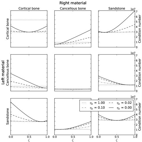
Figure 2 shows the variation of the condition number of the coefficient matrix in (26) as a function of $\zeta$ for various $\eta_{d}$ values and various pairs of materials. The choice of $\zeta$ is essentially irrelevant except for impermeable or nearly impermeable interfaces, and even for these interfaces we see no worse than about a factor of five difference between the lowest and highest condition number for a given material combination — not a significant variation, given that the highest condition number observed is around $7\times 10^{7}$. For similar materials, the minimum condition number occurs near $\zeta=\frac{1}{2}$, and even for very dissimilar materials this value of $\zeta$ yields a condition number substantially below the worst possible. Based on these results, for simplicity we set $\zeta=\frac{1}{2}$ for all further computations, corresponding to equal weighting of both sides in computing $\widehat{\mathbf{q}\cdot\mathbf{n}}$.

Fig. 2: Variation of the condition number of the Riemann solution linear system (26) for interfaces between various pairs of poroelastic materials, as a function of the free parameter $\zeta$. Material properties are given in Table 1. The maximum condition number observed is around $7\times 10^{7}$ — not large enough to endanger accuracy in IEEE double-precision arithmetic.

3.3 Modifications to the high-resolution finite volume scheme

The presence of interfaces between media governed by different PDEs presents a special problem for implementing certain aspects of high-resolution finite volume methods. To explore this in more detail, we first write the full update formula for cell $ij$ from timestep $n$ to $n+1$ on a mapped grid, following (21.12) and (23.11) from [34]:

$$\mbox{$\mathbf{Q}$}_{ij}^{n+1}=\mbox{$\mathbf{Q}$}_{ij}-\frac{\Delta t}{\kappa_{ij}\Delta\xi_{1}}\left(\mathcal{A}^{+}\Delta\mbox{$\mathbf{Q}$}_{i-1/2,j}+\mathcal{A}^{-}\Delta\mbox{$\mathbf{Q}$}_{i+1/2,j}\right)-\frac{\Delta t}{\kappa_{ij}\Delta\xi_{2}}\left(\mathcal{B}^{+}\Delta\mbox{$\mathbf{Q}$}_{i,j-1/2}+\mathcal{B}^{-}\Delta\mbox{$\mathbf{Q}$}_{i,j+1/2}\right)\\ -\frac{\Delta t}{\kappa_{ij}\Delta\xi_{1}}\left(\tilde{\mathbf{F}}_{i+1/2,j}-\tilde{\mathbf{F}}_{i-1/2,j}\right)-\frac{\Delta t}{\kappa_{ij}\Delta\xi_{2}}\left(\tilde{\mathbf{G}}_{i,j+1/2}-\tilde{\mathbf{G}}_{i,j-1/2}\right).$$ (29)

All quantities on the right-hand side are evaluated at timestep $n$. The coordinates $\xi_{1}$ and $\xi_{2}$ are computational coordinates, $\kappa_{ij}$ is the ratio of the area of cell $ij$ to $\Delta\xi_{1}\,\Delta\xi_{2}$, $\mathcal{A}^{+}\Delta\mbox{$\mathbf{Q}$}_{i-1/2,j}$ etc. are the fluctuations computed from the Riemann solutions at the interfaces with neighboring cells, and $\tilde{\mathbf{F}}_{i-1/2,j}$ etc. are the correction fluxes. These correction fluxes are a combination of corrections coming from transverse Riemann solutions, which are important for stability in multi-dimensional problems, and higher-order correction fluxes, which allow the method to achieve second-order accuracy.

It is these correction fluxes that pose a problem here. Because at a fluid-poroelastic interface the solutions in the two domains are governed by different PDEs, it is not possible to construct a single flux transferring quantities from one domain to the other in this form. For example, in the formulation of acoustics we use here, elements 2 through 6 of $\mathbf{Q}$ are identically zero in a fluid, because they correspond to the total stress tensor and solid velocity. The state of stress in a fluid is described completely by the pressure (since we ignore viscosity in an all-fluid medium here), and there is no solid component present to have a velocity, so a flux appropriate to the poroelastic medium would produce nonsensical results if used to update the solution in the fluid. Similarly, a flux appropriate to the fluid would only update the pressure and fluid flow rate in the poroelastic medium, whereas we should in general expect all of the state variables to be updated. We must therefore reformulate (29) to correctly handle a fluid-poroelastic interface.

Because we cannot define a single flux across an interface between media of different types, we instead define two correction fluctuations, one on either side of the interface — instead of a correction flux $\tilde{\mathbf{G}}_{i,j+1/2}$ acting on both cells $(i,j)$ and $(i,j+1)$, we define a $\tilde{\mathbf{G}}^{+}_{i,j+1/2}$ acting on cell $(i,j+1)$ and a $\tilde{\mathbf{G}}^{-}_{i,j+1/2}$ acting on cell $(i,j)$. These fluctuations have a similar meaning to the first-order fluctuations $\mathcal{A}^{\pm}\Delta\mbox{$\mathbf{Q}$}$ — they measure the rate of change of cell averages caused by waves propagating from the interface. The correction fluctuations are not necessarily equal on either side of the interface, but they are compatible in the sense that they arise from the same Riemann problems and respect the underlying physics of both media. In terms of the correction fluctuations, our new update formula derived from (29) is

$$\mbox{$\mathbf{Q}$}_{ij}^{n+1}=\mbox{$\mathbf{Q}$}_{ij}-\frac{\Delta t}{\kappa_{ij}\Delta\xi_{1}}\left(\mathcal{A}^{+}\Delta\mbox{$\mathbf{Q}$}_{i-1/2,j}+\mathcal{A}^{-}\Delta\mbox{$\mathbf{Q}$}_{i+1/2,j}\right)-\frac{\Delta t}{\kappa_{ij}\Delta\xi_{2}}\left(\mathcal{B}^{+}\Delta\mbox{$\mathbf{Q}$}_{i,j-1/2}+\mathcal{B}^{-}\Delta\mbox{$\mathbf{Q}$}_{i,j+1/2}\right)\\ -\frac{\Delta t}{\kappa_{ij}\Delta\xi_{1}}\left(\tilde{\mathbf{F}}^{-}_{i+1/2,j}-\tilde{\mathbf{F}}^{+}_{i-1/2,j}\right)-\frac{\Delta t}{\kappa_{ij}\Delta\xi_{2}}\left(\tilde{\mathbf{G}}^{-}_{i,j+1/2}-\tilde{\mathbf{G}}^{+}_{i,j-1/2}\right).$$ (30)

Note that the new correction fluctuations keep the same sign convention as the old correction fluxes. Also note that for a Riemann problem with an interface condition of the form (24), the solution is not necessarily a function purely of the difference in cell states; we keep the $\mathcal{A}^{\pm}\Delta\mbox{$\mathbf{Q}$}_{i-1/2,j}$ notation for familiarity’s sake, but it should be interpreted as fluctuations arising from a Riemann problem at cell interface $(i-1/2,j)$, not as an operator applied to a difference of states.

The following subsections describe how we compute the correction fluctuations.

3.3.1 Transverse Riemann solution

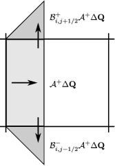
The transverse Riemann solution process computes the contribution of the solution on a cell in one timestep to solutions on the cells diagonally adjacent to it in the next timestep, and is important for stability in a dimensionally-unsplit high-resolution finite volume scheme. Suppose we are considering the contribution to $\mbox{$\mathbf{Q}$}_{ij}^{n+1}$ of the normal Riemann solution at left edge of cell $(i,j)$. Ordinarily, the transverse Riemann solution process would use the right-going fluctuation $\mathcal{A}^{+}\Delta\mbox{$\mathbf{Q}$}_{i-1/2,j}$ to calculate up-going and down-going transverse fluctuations $\mathcal{B}^{+}\mathcal{A}^{+}\Delta\mbox{$\mathbf{Q}$}_{i-1/2,j}$ and $\mathcal{B}^{-}\mathcal{A}^{+}\Delta\mbox{$\mathbf{Q}$}_{i-1/2,j}$. This is illustrated in Figure 3a. In the case of a linear system such as ours, these transverse fluctuations are found by decomposing $\mathcal{A}^{+}\Delta\mbox{$\mathbf{Q}$}_{i-1/2,j}$ into eigenvectors of the flux Jacobians corresponding to the interfaces between cell $(i,j)$ and cells $(i,j-1)$ and $(i,j+1)$, then multiplying by the respective eigenvalues and by the ratio of the physical length of the cell interface to $\Delta\xi_{1}$; the portion of the eigendecomposition corresponding to positive eigenvalues is $\mathcal{B}^{+}\mathcal{A}^{+}\Delta\mbox{$\mathbf{Q}$}_{i-1/2,j}$, while the portion corresponding to negative eigenvalues is $\mathcal{B}^{-}\mathcal{A}^{+}\Delta\mbox{$\mathbf{Q}$}_{i-1/2,j}$. The correction fluxes $\tilde{\mathbf{G}}_{i,j+1/2}$ and $\tilde{\mathbf{G}}_{i,j-1/2}$ are then incremented by $-\frac{\Delta t}{2\Delta\xi_{1}}\mathcal{B}^{+}\mathcal{A}^{+}\Delta\mbox{$\mathbf{Q}$}_{i-1/2,j}$ and $-\frac{\Delta t}{2\Delta\xi_{1}}\mathcal{B}^{-}\mathcal{A}^{+}\Delta\mbox{$\mathbf{Q}$}_{i-1/2,j}$, respectively.

(a) Classical

(b) Fluctuation-based

Fig. 3: Comparison of classical and fluctuation-based approaches to cell updates from transverse Riemann solves. Classical approach: both cells on either side of the transverse interface are updated using the same transverse flux. Fluctuation-based approach: each cell is updated using a separate fluctuation.

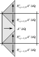
For our new approach, illustrated in Figure 3b, we compute the contributions of the fluctuation $\mathcal{A}^{+}\Delta\mbox{$\mathbf{Q}$}_{i-1/2,j}$ to, for instance, the two distinct correction fluctuations $\tilde{\mathbf{G}}^{\pm}_{i,j-1/2}$ by applying the Riemann solver to the states in cells $(i,j)$ and $(i,j-1)$ modified by the fluctuations from the normal Riemann solve. (For our particular case, we exploit linearity by separately computing the transverse fluctuations from each normal fluctuation, which is the easiest approach to fit into the existing clawpack framework. It would also be possible to reduce computational effort by computing combined transverse fluctuations from the normal fluctuations in cells in two adjacent rows taken together — e.g., computing $\mathcal{A}^{+}\Delta\mbox{$\mathbf{Q}$}_{i-1/2,j}$ and $\mathcal{A}^{+}\Delta\mbox{$\mathbf{Q}$}_{i-1/2,j+1}$, then using them together to compute $\mathcal{B}^{\pm}_{i,j+1/2}$ fluctuations by a process very similar to solving a normal Riemann problem between states $\mathcal{A}^{+}\Delta\mbox{$\mathbf{Q}$}_{i-1/2,j}$ and $\mathcal{A}^{+}\Delta\mbox{$\mathbf{Q}$}_{i-1/2,j+1}$.) We then use the fluctuations $\mathcal{B}^{\pm}\mathcal{A}^{+}\Delta\mbox{$\mathbf{Q}$}_{i-1/2,j}$ from the Riemann solution to increment $\tilde{\mathbf{G}}^{-}_{i,j-1/2}$ by $-\frac{\Delta t}{2\Delta\xi_{1}}\mathcal{B}^{-}\mathcal{A}^{+}\Delta\mbox{$\mathbf{Q}$}_{i-1/2,j}$, and $\tilde{\mathbf{G}}^{+}_{i,j-1/2}$ by $+\frac{\Delta t}{2\Delta\xi_{1}}\mathcal{B}^{+}\mathcal{A}^{+}\Delta\mbox{$\mathbf{Q}$}_{i-1/2,j}$. The other correction fluctuations are updated analogously from transverse Riemann solutions computed at each cell interface.

To compare these two approaches, we write out the full contribution to the update of cell $(i,j)$ of the transverse solves based on the right-going fluctuation from its left edge. To make the difference between the methods clear, we attach a subscript to each transverse fluctuation operator identifying the interface at which it was computed — so, for example, the up-going transverse fluctuation from the upper edge of cell $(i,j)$ is $\mathcal{B}^{+}_{i,j+1/2}\mathcal{A}^{+}\Delta\mbox{$\mathbf{Q}$}_{i-1/2,j}$. The classical transverse solve approach increments cell $(i,j)$ by

$$\Delta\mbox{$\mathbf{Q}$}_{ij,\text{trans},\text{classical}}=-\frac{\Delta t^{2}}{2\kappa_{ij}\Delta\xi_{1}\,\Delta\xi_{2}}\left(-\mathcal{B}^{+}_{i,j+1/2}\mathcal{A}^{+}\Delta\mbox{$\mathbf{Q}$}_{i-1/2,j}+\mathcal{B}^{-}_{i,j-1/2}\mathcal{A}^{+}\Delta\mbox{$\mathbf{Q}$}_{i-1/2,j}\right),$$ (31)

while the new fluctuation-oriented approach increments the cell by

$$\Delta\mbox{$\mathbf{Q}$}_{ij,\text{trans},\text{fluctuation}}=-\frac{\Delta t^{2}}{2\kappa_{ij}\Delta\xi_{1}\,\Delta\xi_{2}}\left(\mathcal{B}^{-}_{i,j+1/2}\mathcal{A}^{+}\Delta\mbox{$\mathbf{Q}$}_{i-1/2,j}-\mathcal{B}^{+}_{i,j-1/2}\mathcal{A}^{+}\Delta\mbox{$\mathbf{Q}$}_{i-1/2,j}\right).$$ (32)

The two approaches produce identical results if the $\mathcal{B}^{\pm}_{i,j+1/2}$ operators are the same as $\mathcal{B}^{\pm}_{i,j-1/2}$, but differ otherwise. Notice that (32) updates the cell using fluctuations computed from waves entering it, while (31) uses fluctuations from waves leaving it, which may not be appropriate. Both approaches produce the same increment to cell $ij$ from the transverse solves applied to the normal fluctuations from the rows above and below, $\mathcal{A}^{+}\Delta\mbox{$\mathbf{Q}$}_{i-1/2,j\pm 1}$.

We make one final note here on the broader applicability of this way of handling transverse propagation, regarding conservation. While we do not cast the governing equations of a fluid-poroelastic system in conservation form, one of the great strengths of high-resolution finite volume methods is their ability to maintain conservation of physically relevant quantities such as mass, momentum, or energy when they are applied to systems of conservation laws. Going from a single transverse flux to a pair of transverse fluctuations appears to jeopardize this — it is not obvious that $\mathcal{B}^{+}_{i,j+1/2}\mathcal{A}^{+}_{i-1/2,j}\Delta\mbox{$\mathbf{Q}$}$ will update cell $(i,j+1)$ by an equal and opposite amount to the update of $\mathcal{B}^{-}_{i,j+1/2}\mathcal{A}^{+}_{i-1/2,j}\Delta\mbox{$\mathbf{Q}$}$ to cell $(i,j)$. Ensuring this happens, though, is very similar to ensuring that the two normal fluctuations $\mathcal{B}^{\pm}\Delta\mbox{$\mathbf{Q}$}$ update neighboring cells in a conservative fashion, so it should be no barrier to practical use. To demonstrate, suppose that we have some general, possibly nonlinear problem. Let $\mathcal{B}^{\pm}(\mbox{$\mathbf{Q}$}_{i,j+1},\mbox{$\mathbf{Q}$}_{ij})$ denote the up-going and down-going fluctuations from the normal Riemann solver applied to states $\mbox{$\mathbf{Q}$}_{i,j+1}$ and $\mbox{$\mathbf{Q}$}_{ij}$ in cells $(i,j+1)$ and $(i,j)$. Assume that for all $i$ and $j$ these fluctuations satisfy the condition

$$\mathcal{B}^{+}(\mbox{$\mathbf{Q}$}_{i,j+1},\mbox{$\mathbf{Q}$}_{ij})+\mathcal{B}^{-}(\mbox{$\mathbf{Q}$}_{i,j+1},\mbox{$\mathbf{Q}$}_{ij})=\mathbf{G}(\mbox{$\mathbf{Q}$}_{i,j+1})-\mathbf{G}(\mbox{$\mathbf{Q}$}_{ij}).$$ (33)

This condition is sufficient to ensure conservation [34]; the function $\mathbf{G}$ will typically be the vertical component of the flux vector of the underlying conservation law, but this is not necessary. In that case, a sufficient condition for the new transverse solution scheme to maintain conservation is to require the output of the transverse Riemann solve to be related to that of the normal Riemann solve by

$$\mathcal{B}^{\pm}_{i,j+1/2}\mathcal{A}^{+}_{i-1/2,j}\Delta\mbox{$\mathbf{Q}$}+\mathcal{B}^{\pm}_{i,j+1/2}\mathcal{A}^{+}_{i-1/2,j+1}\Delta\mbox{$\mathbf{Q}$}\\ =\mathcal{B}^{\pm}(\mbox{$\mathbf{Q}$}_{i,j+1}+\mathcal{A}^{+}_{i-1/2,j+1}\Delta\mbox{$\mathbf{Q}$},\mbox{$\mathbf{Q}$}_{ij}+\mathcal{A}^{+}_{i-1/2,j}\Delta\mbox{$\mathbf{Q}$})-\mathcal{B}^{\pm}(\mbox{$\mathbf{Q}$}_{i,j+1},\mbox{$\mathbf{Q}$}_{ij}).$$ (34)

Essentially, this condition states that the total of the transverse fluctuations should be equal to the difference between the up- and down-going normal fluctuations from the states behind the right-going waves, and the states in front of them.

If condition (34) holds, then summing the transverse fluctuations at interface $(i,j+1/2)$ and rearranging a bit gives us

$$\mathcal{B}^{+}_{i,j+1/2}\mathcal{A}^{+}_{i-1/2,j}\Delta\mbox{$\mathbf{Q}$}+\mathcal{B}^{+}_{i,j+1/2}\mathcal{A}^{+}_{i-1/2,j+1}\Delta\mbox{$\mathbf{Q}$}+\mathcal{B}^{-}_{i,j+1/2}\mathcal{A}^{+}_{i-1/2,j}\Delta\mbox{$\mathbf{Q}$}+\mathcal{B}^{-}_{i,j+1/2}\mathcal{A}^{+}_{i-1/2,j+1}\Delta\mbox{$\mathbf{Q}$}\\ =(\mathbf{G}(\mbox{$\mathbf{Q}$}_{i,j+1}+\mathcal{A}^{+}_{i-1/2,j+1}\Delta\mbox{$\mathbf{Q}$})-\mathbf{G}(\mbox{$\mathbf{Q}$}_{i,j+1}))-(\mathbf{G}(\mbox{$\mathbf{Q}$}_{ij}+\mathcal{A}^{+}_{i-1/2,j}\Delta\mbox{$\mathbf{Q}$})-\mathbf{G}(\mbox{$\mathbf{Q}$}_{ij}))=\mathbf{K}_{i,j+1}-\mathbf{K}_{i,j},$$ (35)

where $\mathbf{K}_{ij}:=\mathbf{G}(\mbox{$\mathbf{Q}$}_{ij}+\mathcal{A}^{+}_{i-1/2,j}\Delta\mbox{$\mathbf{Q}$})-\mathbf{G}(\mbox{$\mathbf{Q}$}_{ij})$. This is precisely analogous to (33), and ensures that the transverse fluctuations will update the solution in a conservative fashion. Condition (34) is typically satisfied by transverse solvers for linear problems (including our own transverse solvers away from interfaces between distinct media, which is the only situation where conservation of the elements of $\mathbf{Q}$ makes sense for our problem), and (34) may be taken as a recipe for defining conservative transverse fluctuations for problems for which it is not immediately obvious how to do so.

3.3.2 Second-order correction term

These terms modify the basic Godunov-type update of the first line of (29) with an additional antidiffusive flux. Mathematically, they provide the second-order terms in the Taylor expansion of the solution in time; qualitatively, they remove the diffusive error from the Godunov update, sharpening the solution. In a classical high-resolution finite volume method, these second-order correction fluxes are computed as linear combinations of the waves propagating from each interface, with limiters applied to each wave. These limiters compare the strength of a wave at an interface to that of the wave in the same family at the neighboring interface in the upwind direction; based on its relative strength the wave may be scaled downward in magnitude to avoid overshoot, or amplified to sharpen the solution. For a more thorough discussion, see chapter 6 of LeVeque [34].

There are two problems with implementing appropriate second-order correction fluxes here. The first is in formulating the appropriate numerical flux function on either side of an interface where a condition of the form (24) holds. This is not trivial, but can be accomplished with, for instance, an approach based on the Immersed Interface Method [35, 41, 42]. The second, harder problem is in creating an appropriate limiting scheme when the waves in the upwind direction are in a different medium and may be in no way analogous to the waves we wish to limit.

Because of these problems, we omit the second-order correction term at interfaces between different materials. While this reduces the accuracy of our solution to first order locally, we note that classical high-resolution finite volume methods also lose formal accuracy at such interfaces, even if the correction term is included (Section 9.12 of [34]), and that it is only at interfaces between different materials that we incur higher error. At cell interfaces between identical materials, we use the standard second-order correction flux.

3.4 Source term

As in our previous work [33], we handle the source term $\mathbf{D}$$\mathbf{Q}$ in (2) using operator splitting. Based on the our experience with Godunov and Strang splitting, we use only Strang splitting here. The matrix $\mathbf{D}$ has a simple eigenstructure, so we use the exact solution operator $\exp(\mbox{$\mathbf{D}$}\Delta t)$ to advance the solution under the action of the dissipation term; this has the advantages of being the most accurate method available to apply the source term, and of being unconditinally stable for all $\Delta t$. We found in [33] that even Strang splitting degrades to first-order accuracy in the stiff regime where the timestep is longer than the characteristic dissipation time, but for short timesteps it displays the expected second-order behavior.

3.5 Numerical software

We implemented the numerical solution techniques described here using the clawpack finite volume method package, version 4.6 [40]. Normally, writing a clawpack application would require only writing a few plug-in subroutines, such as the Riemann solver; because of our modified formulation, we also had to modify some of its internal subroutines, but using clawpack still greatly reduced the time and effort required for coding compared to starting from scratch. The package supports operator splitting for source terms, such as the dissipative term here, by means of a user-supplied subroutine that advances the system by a specified time step under the action of the source term. Both Godunov and Strang splitting are available, though we use only Strang splitting here. Block-structured Berger-Colella-Oliger adaptive mesh refinement (AMR) is available from the amrclaw package [2]; amrclaw can also run in parallel on shared-memory systems using OpenMP.

4 Results for rectilinear grids

In this section we test our code’s ability to correctly model interfaces between different poroelastic materials, and between a poroelastic material and a fluid, on a rectilinear grid. Note that although the grid lines are straight, these results still use the mapped-grid solver; the grid mapping just happens to be particularly simple. For all cases in this section, we choose the simulation time step such that the global maximum CFL number is 0.9. We also use no limiters anywhere in these simulations — while limiters improve solution accuracy on typical grids, they obscure the convergence behavior of the underlying wave propagation method, which is what we seek to observe here. Since the solutions used in this section are smooth except at interfaces between different media, we will not encounter serious trouble from the numerical dispersion that limiters are designed to suppress. Table 1 lists the properties of all the materials used here.

Table 1: Properties of the poroelastic media used in test cases. Stone properties are taken from de la Puente et al. [16]; bone properties are from [13, 28, 29, 39]. Cortical bone properties refer to vascular pore space. The sandstone properties are orthotropic, but the other materials are isotropic. Wave speeds are correct in the high-frequency limit. $c_{pf}$ is the fast P wave speed, $c_{s}$ is the S wave speed, $c_{ps}$ is the slow P wave speed, and $\tau_{d}$ is the time constant for dissipation. Subscript numbers indicate principal directions.

		Sandstone	Shale	Cortical bone	Cancellous bone
Base properties
$K_{s}$	(GPa)	80	7.6	14	18.5
$\rho_{s}$	(kg/m3)	2500	2210	1960	1960
$c_{11}$	(GPa)	71.8	11.9	20.6	5.2
$c_{12}$	(GPa)	3.2	3.96	10.6	2.4
$c_{13}$	(GPa)	1.2	3.96	10.6	2.4
$c_{33}$	(GPa)	53.4	11.9	20.6	5.2
$c_{55}$	(GPa)	26.1	3.96	5	1.38
$\phi$		0.2	0.16	0.04	0.75
$\kappa_{1}$	($10^{-15}$ m2)	600	100	630	$7\times 10^{6}$
$\kappa_{3}$	($10^{-15}$ m2)	100	100	630	$7\times 10^{6}$
$T_{1}$		2	2	2	1
$T_{3}$		3.6	2	2	1
$K_{f}$	(GPa)	2.5	2.5	2.3	2.2
$\rho_{f}$	(kg/m3)	1040	1040	1060	990
$\eta$	($10^{-3}$ kg/m$\cdot$s)	1	1	1	40
Derived quantites
$c_{pf1}$	(m/s)	6000	2480	3290	3260
$c_{pf3}$	(m/s)	5260	2480	3290	3260
$c_{s1}$	(m/s)	3480	1430	1620	1680
$c_{s3}$	(m/s)	3520	1430	1620	1680
$c_{ps1}$	(m/s)	1030	1130	1123	1480
$c_{ps3}$	(m/s)	746	1130	1123	1480
$\tau_{d1}$	($\mu$s)	5.95	1.25	33	92
$\tau_{d3}$	($\mu$s)	1.82	1.25	33	92

The results we wish to show in this section are error values and convergence rates. Where we measure error relative to the true solution, we do so using grid energy norms: we take the energy norm (defined by (12)) of the difference between the numerical solution for each grid cell and the true solution evaluated at the cell centroid. We then define the 1-norm and max-norm errors as

error 1-norm $$=\frac{1}{N_{1}N_{2}}\sum_{i=1}^{N_{1}}\sum_{j=1}^{N_{2}}\|\mbox{$\mathbf{Q}$}_{ij,\text{numerical}}-\mbox{$\mathbf{Q}$}_{ij,\text{true}}\|_{E}$$ (36)

error max-norm $$=\max_{i,j}\|\mbox{$\mathbf{Q}$}_{ij,\text{numerical}}-\mbox{$\mathbf{Q}$}_{ij,\text{true}}\|_{E}$$

where $N_{1}$ and $N_{2}$ are the grid dimensions in the two computational axes. The incident waves are all scaled to unit peak energy density, so these grid energy error norms provide an overall measure of relative error in the numerical solution, with the various components of the solution scaled appropriately relative to each other. All cases in this section test the ability of the code to correctly evolve a known analytical solution: we initialize all simulations by evaluating the true solution at cell centroids, and boundary conditions are implemented using the standard ghost cell approach, with ghost cells filled using the true solution evaluated at ghost cell centroids. In addition, all the solutions considered in this section are periodic in time. We have observed that in such cases the error in the numerical solution displays a periodic component, which gives it local minima at integer multiples of the period after the starting time, so to avoid artificially picking the best result we evaluate the solution error after 1.25 periods. Since we run a very large number of simulations, we do not display convergence using plots of error versus grid size or spacing. Instead, for each true solution we perform a linear least-squares fit of the logarithm of error in each norm with respect to the logarithm of grid dimension; we report the best, worst, and mean convergence rates across all solutions, as measured by the slopes of these fit lines, along with the worst $R^{2}$ value for the fit, and the best and worst errors in each norm on the finest grid used. For all test cases in this section, we assess convergence using grid dimensions of $100\times 100$, $200\times 200$, $400\times 400$, and $800\times 800$ cells.

Before we treat material interfaces on rectilinear grids, we will first explore the consequences of omitting the second-order correction term along a line of cell interfaces.

4.1 Effect of omitting the second-order correction term

To see the results of omitting the second-order correction term, we use time-harmonic simple plane waves propagating in homogeneous media. The correction term is omitted for the vertical-direction fluxes along one grid line passing horizontally through the center of the domain. We examine the results both for poroelastic waves of all three families — though with viscosity omitted, to isolate the effect of the missing term — and for acoustic waves; the material used is the orthotropic sandstone of Table 1 for the poroelastic waves, or just the brine contained within it for acoustic waves. To test grid alignment and transverse solve effects, we vary the wave propagation direction from straight down in the $-z$ direction to $7.5^{\circ}$ clockwise of the $+x$ direction, in $7.5^{\circ}$ increments. Because the sample poroelastic material is orthotropic, we also vary its principal $1$-direction from horizontal to $165^{\circ}$ counterclockwise of horizontal, in $15^{\circ}$ increments. We omit the viscous dissipation term for the poroelastic waves, since we wish to focus on error in the wave-propagation part of the algorithm; since these tests are inviscid, the period of the wave and time required to cross the domain are the only time scales present, so we choose an angular frequency of 1 rad/s. For all cases, the computational domain is a square whose side length is two wavelengths of a wave in the incident family propagating in the material principal $1$-direction.

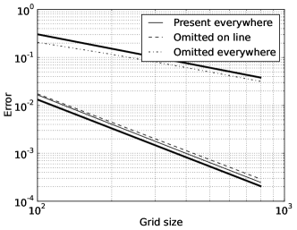
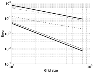
Table 2 shows the results of this convergence study. Even with the second-order correction term omitted along a line, we still obtain second-order convergence in the 1-norm. Convergence degrades to first-order (typically) or somewhat below (in the worst case) for the max-norm. These results are about as good as could be expected from omitting the second-order term. Figure 4 examines in greater detail the case that gives the worst error on the $800\times 800$ grid — a slow P wave propagating vertically downward, with the principal direction of the poroelastic sandstone medium oriented $15^{\circ}$ counterclockwise of horizontal. In the 1-norm, results are almost as good as if the second-order correction term were present everywhere, while in the max-norm, even though the convergence rate is reduced to first-order when the term is omitted along a line, the magnitude of the error is almost four times less than if it were omitted everywhere. This suggests that we can expect results of reasonable accuracy even with the second-order correction term omitted at interfaces between different media.

Table 2: Convergence results for acoustic and inviscid poroelastic waves with the second-order correction term omitted along a line of cell interfaces.

		Convergence rate				Error on $800\times 800$ grid
	Error norm	Best	Worst	Mean	Worst $R^{2}$ value	Best	Worst
Acoustic	1-norm	2.01	1.99	2.00	0.99957	$2.57\times 10^{-5}$	$4.09\times 10^{-5}$
	Max-norm	1.49	1.03	1.15	0.95837	$2.76\times 10^{-4}$	$2.51\times 10^{-3}$
Fast P	1-norm	2.02	1.97	1.99	0.99883	$2.75\times 10^{-5}$	$7.83\times 10^{-5}$
	Max-norm	1.45	0.91	1.13	0.86779	$4.62\times 10^{-4}$	$3.74\times 10^{-3}$
S	1-norm	2.01	1.98	1.99	0.99999	$4.18\times 10^{-5}$	$9.49\times 10^{-5}$
	Max-norm	1.76	0.95	1.15	0.96214	$4.05\times 10^{-4}$	$5.06\times 10^{-3}$
Slow P	1-norm	2.01	1.95	1.98	0.99999	$8.21\times 10^{-5}$	$3.10\times 10^{-4}$
	Max-norm	1.85	0.76	1.09	0.98524	$9.91\times 10^{-4}$	$1.99\times 10^{-2}$

(a) 1-norm

(b) Max-norm

Fig. 4: Detailed examination of the effect of omitting the second-order correction term for the case of Table 2 that had the highest error on the finest grid. Results of omitting the second-order correction term on a line are compared to results if the term is present or omitted everywhere. The thick black lines are first- and second-order reference lines.

4.2 Reflected and transmitted waves at a fluid-poroelastic interface

To test our code’s ability to correctly handle material interfaces, we first examine the case of a time-harmonic plane acoustic wave striking a flat interface between a poroelastic medium and a fluid. In all cases, the interface between the two media is horizontal, and the incident wave impinges from the top side. Figure 5a shows a simple sketch of the problem. We generate analytical solutions for these cases using the procedure described in Appendix B. The poroelastic medium used is the brine-saturated sandstone of Table 1, and the fluid medium is the same brine contained in the sandstone. We again perform a combinatorial sweep over the relevant parameters. In this case, we vary the direction of the incident wave from $7.5^{\circ}$ below horizontal to straight down in $7.5^{\circ}$ increments, and the principal material $1$-direction from horizontal to $165^{\circ}$ counterclockwise of horizontal in $15^{\circ}$ increments. For each combination of incident wave and material principal directions, we simulate with interface discharge efficiencies $\eta_{d}$ of $0$ (sealed pores), $0.5$ (imperfect hydraulic contact), and $1$ (open pores). The dimensions of the domain are two wavelengths of an acoustic wave at the chosen frequency. We perform these tests both with viscosity ignored, in order to investigate the performance of the hyperbolic solver by itself, and with viscosity included. For the inviscid tests, since the period of the wave and time required for it to cross the domain are the only time scales present, the wave frequency is not directly relevant to the solution error, so we chose an angular frequency of $1$ rad/s. With viscosity included, the dissipation term has its own intrinsic time scale indepdendent of the wave behavior, so choice of frequency is important. For these viscous tests, we restrict ourselves to a high frequency (10 kHz; the maximum frequency for validity of Biot theory in the sandstone medium is 25 kHz), because at low frequencies the slow P wave dissipates over distances much shorter than a wavelength. In fact, the characteristic decay length is much shorter than the grid spacing on an otherwise reasonably resolved grid, so at low frequencies the transmitted slow P wave could not be resolved without refining the grid to impractical levels. This also results in grid sizes and corresponding time steps short enough that these models are outside the stiff regime identified in [33]. For all cases, the computational domain is again a square with side length equal to two wavelengths of incident acoustic wave.

(a) Fluid-poroelastic

(b) Poroelastic-poroelastic

Fig. 5: Simple sketches of reflection/transmission problems used to test convergence. The incident, reflected, and transmitted waves are labeled by type; an incident poroelastic wave may be of any of the three types.

Tables 3 and 4 show the results of these convergence studies for the inviscid and viscous high-frequency tests respectively. We obtain second-order convergence for all cases in the 1-norm, though results are degraded to first-order in the max-norm due to the omission of the second-order correction term at the interface, as expected from the results of the previous section. All three interface conditions (open and sealed pores, and imperfect hydraulic contact) show similar levels of error, and the difference between best and worst error obtained in the finest grid is also not large. Convergence rates are slightly worse for the viscous cases; they are still typically quite close to the expected second-order and first-order results, but some outlying cases degrade as far as order 0.7, possibly due to the compounding of first-order error at the interface with operator splitting error.

Table 3: Convergence results for an acoustic wave impinging on sandstone, with viscosity omitted.

		Convergence rate				Error on $800\times 800$ grid
	Error norm	Best	Worst	Mean	Worst $R^{2}$ value	Best	Worst
$\eta_{d}=0$	1-norm	2.00	1.98	1.99	1.00000	$7.93\times 10^{-5}$	$2.09\times 10^{-4}$
	Max-norm	1.50	0.88	1.12	0.96350	$2.17\times 10^{-3}$	$1.25\times 10^{-2}$
$\eta_{d}=0.5$	1-norm	2.01	1.97	1.99	0.99999	$1.03\times 10^{-4}$	$2.94\times 10^{-4}$
	Max-norm	1.47	0.88	1.14	0.95713	$2.12\times 10^{-3}$	$1.24\times 10^{-2}$
$\eta_{d}=1$	1-norm	2.01	1.97	2.00	0.99999	$1.07\times 10^{-4}$	$3.14\times 10^{-4}$
	Max-norm	1.52	0.88	1.15	0.95981	$2.16\times 10^{-3}$	$1.24\times 10^{-2}$

Table 4: Convergence results for a $10$ kHz acoustic wave impinging on sandstone, with viscosity included.

		Convergence rate				Error on $800\times 800$ grid
	Error norm	Best	Worst	Mean	Worst $R^{2}$ value	Best	Worst
$\eta_{d}=0$	1-norm	1.99	1.96	1.98	1.00000	$6.93\times 10^{-5}$	$1.21\times 10^{-4}$
	Max-norm	1.44	0.88	1.09	0.96397	$2.46\times 10^{-3}$	$1.25\times 10^{-2}$
$\eta_{d}=0.5$	1-norm	1.97	1.90	1.95	0.99999	$6.84\times 10^{-5}$	$1.79\times 10^{-4}$
	Max-norm	1.30	0.72	0.98	0.97612	$2.96\times 10^{-3}$	$2.06\times 10^{-2}$
$\eta_{d}=1$	1-norm	1.97	1.90	1.94	0.99999	$6.75\times 10^{-5}$	$1.83\times 10^{-4}$
	Max-norm	1.29	0.70	0.98	0.97672	$3.02\times 10^{-3}$	$2.19\times 10^{-2}$

4.3 Reflected and transmitted waves at an interface between two poroelastic materials

We also examine plane waves reflected and transmitted at an interface between two poroelastic media. For these cases the upper medium is the isotropic, brine-saturated shale of Table 1, and the lower medium is again orthotropic sandstone; Figure 5b shows a simple sketch of the reflected and transmitted waves in this case. These cases are quite similar to the fluid-poroelastic cases, with the exception that we send in incident waves in multiple different poroelastic wave families. To reduce the total number of cases, we run a smaller number of incident wave directions — we vary the angle of incidence from $7.5^{\circ}$ below horizontal to $82.5^{\circ}$ in steps of $15^{\circ}$, which halves the number of angles of incidence and drops the relatively uninteresting normal incidence, while retaining the grazing $7.5^{\circ}$ angle. We use the same set of principal material directions for the sandstone as in the fluid-poroelastic cases; principal material direction is irrelevant for the shale because it is isotropic. We also use the same sets of interface discharge efficiencies and grid dimensions. For all cases the domain size is two wavelengths of the fast P wave in shale at the chosen frequency. The inviscid cases use waves with an angular frequency of 1 rad/s, while the viscous cases use 20 kHz waves, a frequency high enough to be out of the stiff regime (or just at the edge of it in shale for a $100\times 100$ grid) but low enough for low-frequency Biot theory to be valid for both materials. We simulate incident waves in all three families for the inviscid cases in order to exercise all different possibilities in the solution code, but with viscosity present we do not include incident slow P waves — their decay rate is high enough that their amplitude is reduced by a factor of $10^{20}$ over the width of the domain, making these cases both intractable to simulate and unrealistic.

Tables 5 and 6 show the results of these convergence studies. Similarly to the acoustic-poroelastic cases, we obtain consistent second-order convergence in the 1-norm, and first-order or better convergence in the max-norm. This occurs for all incident wave types, even in the face of the operator splitting error present in the viscous cases. In fact, the worst-case convergence rates are better than for the acoustic-poroelastic cases, perhaps due to a more tractable interface condition.

Table 5: Convergence results for poroelastic waves in shale impinging on sandstone, with viscosity omitted.

	Incident wave		Convergence rate			Worst $R^{2}$ value	Error on $800\times 800$ grid
		Error norm	Best	Worst	Mean		Best	Worst
$\eta_{d}=0$	Fast P	1-norm	2.01	1.99	2.00	1.00000	$8.81\times 10^{-5}$	$3.26\times 10^{-4}$
		Max-norm	1.49	1.06	1.17	0.97570	$2.01\times 10^{-3}$	$5.62\times 10^{-3}$
	S	1-norm	2.01	1.98	1.99	0.99999	$2.19\times 10^{-4}$	$4.27\times 10^{-4}$
		Max-norm	1.86	1.03	1.25	0.98292	$2.39\times 10^{-3}$	$1.18\times 10^{-2}$
	Slow P	1-norm	2.00	1.99	2.00	0.99999	$3.34\times 10^{-4}$	$6.34\times 10^{-4}$
		Max-norm	1.92	1.08	1.40	0.99555	$3.90\times 10^{-3}$	$2.13\times 10^{-2}$
$\eta_{d}=0.5$	Fast P	1-norm	2.00	1.98	1.99	1.00000	$7.65\times 10^{-5}$	$2.00\times 10^{-4}$
		Max-norm	1.22	1.01	1.13	0.99179	$1.99\times 10^{-3}$	$5.63\times 10^{-3}$
	S	1-norm	2.01	1.98	1.99	0.99999	$2.13\times 10^{-4}$	$3.49\times 10^{-4}$
		Max-norm	1.86	0.99	1.24	0.98301	$2.38\times 10^{-3}$	$1.18\times 10^{-2}$
	Slow P	1-norm	2.01	1.99	2.00	0.99999	$4.70\times 10^{-4}$	$1.44\times 10^{-3}$
		Max-norm	1.99	1.06	1.40	0.96976	$3.81\times 10^{-3}$	$1.96\times 10^{-2}$
$\eta_{d}=1$	Fast P	1-norm	2.00	1.99	1.99	1.00000	$7.66\times 10^{-5}$	$1.99\times 10^{-4}$
		Max-norm	1.22	1.00	1.13	0.99181	$1.99\times 10^{-3}$	$5.63\times 10^{-3}$
	S	1-norm	2.01	1.98	1.99	0.99999	$2.11\times 10^{-4}$	$3.49\times 10^{-4}$
		Max-norm	1.86	0.98	1.24	0.98301	$2.38\times 10^{-3}$	$1.18\times 10^{-2}$
	Slow P	1-norm	2.01	1.99	2.00	0.99999	$4.86\times 10^{-4}$	$1.50\times 10^{-3}$
		Max-norm	1.99	1.05	1.41	0.97068	$3.86\times 10^{-3}$	$1.98\times 10^{-2}$

Table 6: Convergence results for 20 kHz poroelastic waves in shale impinging on sandstone, with viscosity included.

	Incident wave		Convergence rate			Worst $R^{2}$ value	Error on $800\times 800$ grid
		Error norm	Best	Worst	Mean		Best	Worst
$\eta_{d}=0$	Fast P	1-norm	2.00	1.96	1.99	1.00000	$6.97\times 10^{-5}$	$1.80\times 10^{-4}$
		Max-norm	1.21	1.01	1.12	0.99164	$1.98\times 10^{-3}$	$5.88\times 10^{-3}$
	S	1-norm	2.01	1.98	1.99	1.00000	$2.10\times 10^{-4}$	$4.40\times 10^{-4}$
		Max-norm	1.86	1.02	1.25	0.97550	$2.56\times 10^{-3}$	$1.20\times 10^{-2}$
$\eta_{d}=0.5$	Fast P	1-norm	2.00	1.97	1.99	1.00000	$6.99\times 10^{-5}$	$1.81\times 10^{-4}$
		Max-norm	1.21	1.01	1.12	0.99168	$1.98\times 10^{-3}$	$5.78\times 10^{-3}$
	S	1-norm	2.01	1.99	1.99	0.99999	$2.09\times 10^{-4}$	$4.43\times 10^{-4}$
		Max-norm	1.86	1.02	1.25	0.97509	$2.53\times 10^{-3}$	$1.20\times 10^{-2}$
$\eta_{d}=1$	Fast P	1-norm	2.00	1.97	1.99	1.00000	$7.00\times 10^{-5}$	$1.81\times 10^{-4}$
		Max-norm	1.21	1.01	1.12	0.99169	$1.98\times 10^{-3}$	$5.78\times 10^{-3}$
	S	1-norm	2.01	1.99	1.99	0.99999	$2.09\times 10^{-4}$	$4.43\times 10^{-4}$
		Max-norm	1.86	1.02	1.25	0.97510	$2.53\times 10^{-3}$	$1.20\times 10^{-2}$

5 Results for curved interfaces and mapped grids

Now that we have examined the convergence behavior of our code for problems with interfaces on rectilinear grids, we turn to curvilinear mapped grids. Here we treat two types of problem. First, we perform a convergence study for a time-harmonic plane wave scattering off an isotropic poroelastic cylinder — a case for which we have an analytic solution — and second, we simulate an acoustic pulse striking a simplified model of a human femur bone.

5.1 Cylindrical scatterer

We model a cylindrical scatterer composed of the isotropic shale of Table 1. Our reference solution is for a time-harmonic acoustic plane wave scattering off a cylindrical isotropic poroelastic body; we obtained it by transforming the poroelastic-acoustic system into a set of coupled Helmholtz equations, then expressing their solutions as bi-infinite series of Bessel and Hankel function modes. This solution is very similar to that of Laperre and Thys [32], although we extend it to imperfect hydraulic contact in addition to open or closed pores. It has a variety of interesting properties, including resonance-like behavior at certain frequencies; we plan a companion publication exploring its properties in more detail. For now, we confine ourselves to a specific model — a shale cylinder 5 cm in diameter, in a bath of fluid identical to its pore fluid.

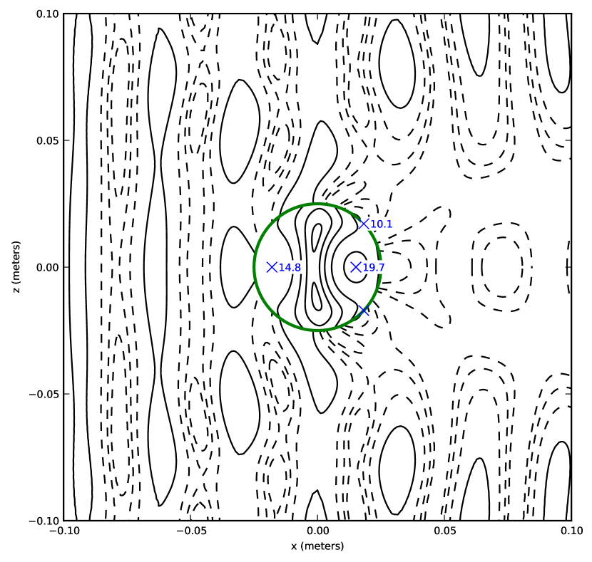
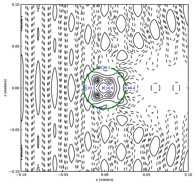
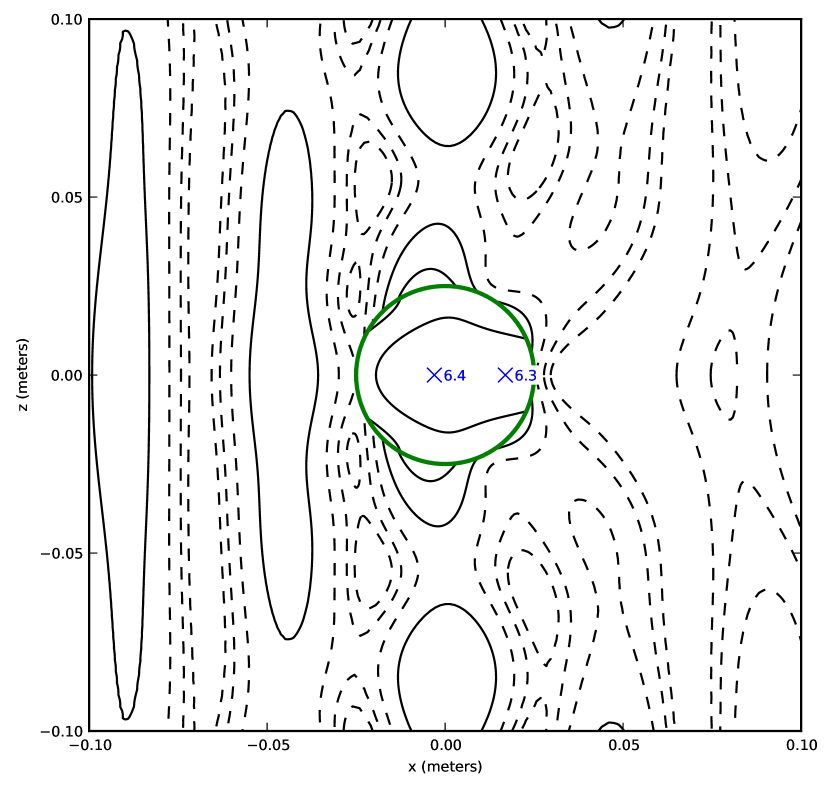
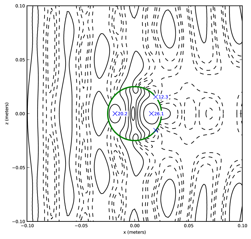
In order to choose sensible input frequencies in the face of the complex behaivor of the analytical solution, we first examine the average energy contained in the cylinder over one cycle as a function of frequency, normalized by the average energy contained in the incident wave over the same volume and time. The required integral of the solution in the radial direction is not readily computable analytically, so we use Romberg quadrature instead, applied recursively until the relative difference between the highest-order iterates at successive depths is less than $10^{-9}$. We also truncate the series solution to 35 terms in each direction, by which index the series terms have decreased to $10^{-9}$ or less of their typical magnitudes for low index at all frequencies below the Biot low-frequency validity cutoff, and are decaying rapidly. Figure 6 shows this normalized average energy content with and without viscosity, for open, sealed, and imperfect pore conditions. Based on this frequency response plot, we selected three frequencies that showed strong response for each combination of viscosity and interface permeability to test the convergence of our code. We chose these strongly-responding frequencies because they would be a more rigorous test of our numerical model: the solution is large within the cylinder, coinciding with the most distorted grid cells, and accurate handling of the transfer of energy and momentum across the interface is likely to be more important. Table 7 lists the cases chosen, and Figure 8 plots the energy density at the initial time for two selected cases. Similar plots for all cylindrical scatterer cases can be found in Appendix C.

Fig. 6: Frequency response plot for 5 cm diameter cylindrical scatterer composed of shale, with and without viscosity, for several interface discharge efficiencies $\eta_{d}$. The vertical axis is ratio of the average energy contained within the cylinder over one cycle to the average energy contained within an equal volume of the undisturbed incident wave. The circles indicate cases chosen for convergence evaluation of the mapped-grid poroelastic/fluid code. This plot goes up to a maximum frequency of one-third of the cutoff frequency for validity of low-frequency Biot theory; there is no barrier to modeling all the way up to the cutoff frequency, but the response curve becomes increasingly complicated beyond the portion shown here.

Table 7: Cylindrical scatterer cases chosen for convergence analysis. Note that the reference to “high” frequency here is relative to the scale of Figure 6; all cases are well below the cutoff frequency for validity of low-frequency Biot theory.

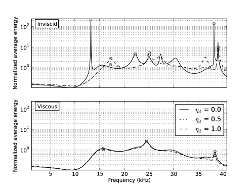
	Inviscid case frequency (kHz)				Viscous case frequency (kHz)
	Low	Mid	High		Low	Mid	High
$\eta_{d}=0$	13.25	22.25	38.20		15.70	24.55	38.39
$\eta_{d}=0.5$	17.25	25.02	39.03		15.80	24.54	38.35
$\eta_{d}=1$	17.30	25.09	39.04		15.80	24.54	38.35

The grid mapping used here deserves some discussion. It is closely related to the square-to-circle mappings of Calhoun, Helzel, and LeVeque [8], but the function defining the radius of curvature of the grid lines has been modified to improve solution quality. Based on experimentation, having concentric grid lines near the surface of the scatterer seems to reduce error, as does having as little grid line curvature as possible and as even a cell size as possible in the interior of the scatterer. Using these considerations as a guide, in the notation of Section 3.2 of [8] our grid mapping is defined by $D(d)=r_{1}d/\sqrt{2}$, $R(d)=r_{1}\left(\frac{9}{10}+d^{19}-\frac{9}{10}d^{20}\right)$. This mapping has $R^{\prime}(1)=r_{1}$ and $R^{\prime\prime}(1)=0$, giving very nearly concentric grid lines near the scatterer surface, and maintains a grid line radius of curvature of $\frac{9}{10}r_{1}$ or greater throughout the interior of the scatterer; the small variation in radius of curvature also helps keep the cell size relatively uniform. Note that even with these modifications, any grid of this type must contain some highly distorted cells, so it should be viewed as one of the worst reasonable cases that might be encountered. Figure 7a shows the mapping in action on a coarse grid.

(a) Cylindrical scatterer

(b) Femur model

Fig. 7: Grid mappings used for cylindrical scatterer and femur models, illustrated on a grid $120\times 120$ cells in total size. The thick green circles denote material boundaries. Only the upper-right quadrant of the distorted region is shown; the grid is rectilinear above and to the right of the region shown, while the parts below and to the left are reflections of the upper-right quadrant.

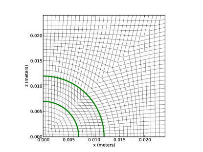
For each case in Table 7, we simulate for 1.25 cycles of the solution, with initial and boundary conditions set using the true solution as in the previous section. The time step is again chosen so that the global maximum CFL number is 0.9. We continue to measure error using the grid energy 1- and max-norms, but since the grid is not uniform we use an area-weighted grid energy 1-norm, computed as

$$\text{error 1-norm}=\frac{\sum_{i=1}^{N_{1}}\sum_{j=1}^{N_{2}}\kappa_{ij}\|\mbox{$\mathbf{Q}$}_{ij,\text{numerical}}-\mbox{$\mathbf{Q}$}_{ij,\text{true}}\|_{E}}{\sum_{i=1}^{N_{1}}\sum_{j=1}^{N_{2}}\kappa_{ij}},$$ (37)

where $N_{1}$ and $N_{2}$ are the numbers of grid cells in the computational $\xi_{1}$ and $\xi_{2}$ directions, and $\kappa_{ij}$ is the cell area ratio discussed in Section 3.1. This is meant to mimic the spatial average of the energy norm of the error. The simulation domain is a square 20 cm on a side, with the cylinder placed at the center. Since the grid mapping is simplest if we use grid dimensions that are a multiple of eight (the ratio of total domain size to cylinder radius), and since the smaller number of cases encourages us to devote more computing resources to each one, we increase the grid sizes used to test convergence to $128\times 128$, $256\times 256$, $512\times 512$, and $1024\times 1024$.

(a) Inviscid, $\eta_{d}=0$, 13.25 kHz, analytical

(b) Viscous, $\eta_{d}=1$, 38.35 kHz, analytical

(c) Inviscid, $\eta_{d}=0$, 13.25 kHz, numerical

(d) Viscous, $\eta_{d}=1$, 38.35 kHz, numerical

Fig. 8: Contour plots of energy density for the analytical solutions of selected test cases from Table 7 at time $t=0$, and the numerical solution on a $1024\times 1024$ grid after one cycle. Values are normalized by peak energy density of incident wave. Contours are placed at every power of 2, with dashed contours indicating negative powers; the lowest solid contour is at unit normalized energy density, with the adjacent dashed contour at $\frac{1}{2}$ and the adjacent solid contour at 2. The thick circle is the boundary of the cylinder. Maximum normalized energy densities inside the cylinder in the upper-left plot are 967 at the left edge, and 929 at the right. The numerical solutions closely match the analytical ones. Similar plots for the analytical solutions for all cases can be found in Appendix C.

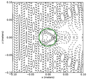
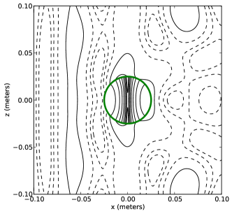
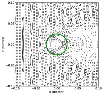
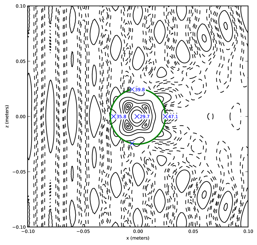
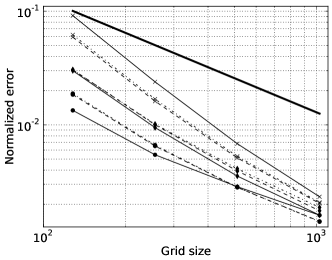
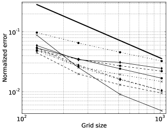
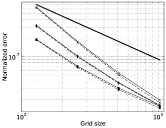
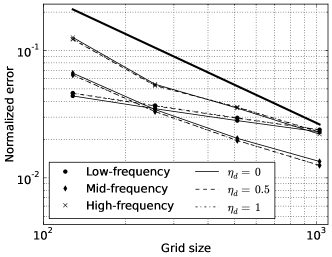
Figure 9 shows the results of these convergence tests. Convergence rates are degraded relative to the rectilinear grid results of Section 4.2. We achieve roughly first-order convergence at large grid sizes in the 1-norm, with faster convergence on coarser grids; in the max-norm, due to the compounding of error due to the nonsmooth grid mapping with operator splitting error and the omission of the second-order correction term at the surface of the scatterer, we typically achieve below first-order convergence, in some cases as low as order $\frac{1}{2}$. Relative errors on the finest grid are typically a few tenths of a percent in the 1-norm, and a few percent in the max-norm. The culprits for these poor convergence results are the highly-distorted, nearly triangular grid cells where the $45^{\circ}$ diagonals intersect the surface of the scatterer. These cells have very high error compared to all other cells in the model; moreover, any logically rectangular grid mapping of this type must produce such cells when it maps a rectangle on the computational grid to a circle on the physical grid. A polar grid could be used instead, but it would introduce difficulties at the pole, and would be difficult to generalize to model multiple scatterers or other additional geometry features. In future work, these problems might be ameliorated somewhat by aggressive use of adaptive mesh refinement — even though the convergence rate is slow, the error on these corner cells still decreases as the grid is refined, and heavy grid refinement could still have a reasonable computational cost if it is restricted to the vicinity of a few problem cells. Despite these problems, however, the bottom half of Figure 8 shows that on a fine grid, after one cycle of the periodic solution, the numerical solution returns very close to its proper value, without any significant artifacts visible. (Note that the numerical solutions shown in the figure were computed using the MC limiter, as opposed to the convergence results, which were computed without any limiter. The limiter was included because its use would be more typical for solving a problem whose solution is not already known.)

(a) 1-norm error for inviscid cases

(b) Max-norm error for inviscid cases

(c) 1-norm error for viscous cases

(d) Max-norm error for viscous cases

Fig. 9: Convergence behavior of cylindrical scatterer test cases. The thick black line is a first-order reference line. Error is normalized by the corresponding norm of the true solution on the computational grid.

5.2 Femur model

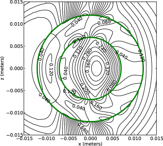
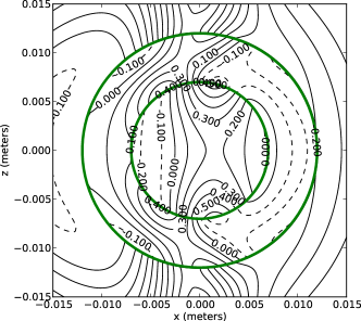
With the results of the previous sections providing reason to be confident in the accuracy of our code, we now turn to a model of a biological system. Specifically, we examine a highly simplified model of an adult human femur bone. This model is composed of an inner cylinder of marrow-filled cancellous bone of radius 7 mm, surrounded by a concentric cylindrical shell of cortical bone 5 mm thick. The outer shell is in turn surrounded by a fluid bath, with both the inner and outer walls of the shell taken to be impermeable to fluid flow. The properties used for both types of bone material are given in Table 1; the fluid bath is taken to be water with bulk modulus $2.25\,\text{GPa}$ and density $1000\,\text{kg}/\text{m}^{3}$. The initial condition is an acoustic pulse traveling in the $+x$ direction toward the bone. The pulse has a Gaussian profile with frequency width 100 kHz, and starts with its peak 15 mm away from the surface. While the pulse frequency width is well beyond the low-frequency Biot cutoff frequency, we intend this as a demonstration example only, as opposed to an accurate quantitative model. Since our model is linear, we give the incoming pulse a peak pressure of 1 Pa for simplicity. We model this concentric cylindrical geometry using a modification of the grid mapping used for the cylindrical scatterer, with the grid lines chosen to be concentric circles between the inner and outer radius of the cortical bone shell. Figure 7b shows the mapping on a coarse grid. The actual computational grid is $800\times 800$ cells. We use simple zero-order extrapolation to implement nonreflecting boundary conditions; the simulation time is too short for significant interaction between the reflected and transmitted waves from the bone and the boundaries of the domain in any case. Since, unlike the other test cases in this work, we are not attempting to isolate the convergence behavior of the wave-propagation algorithm here, we used the monotonized centered limiter for all waves in this computation.

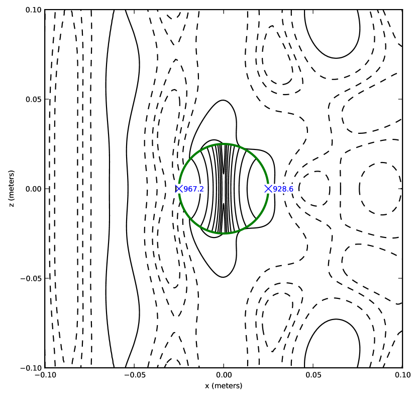
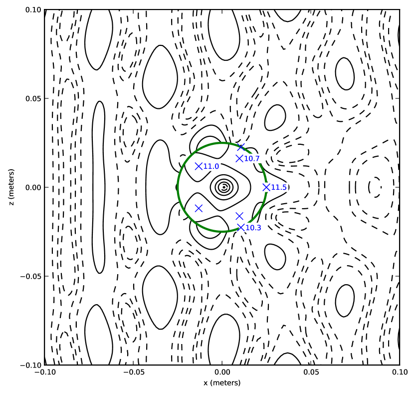
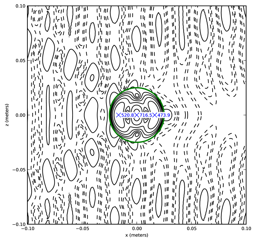
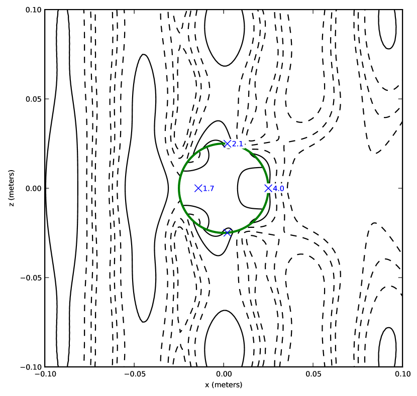
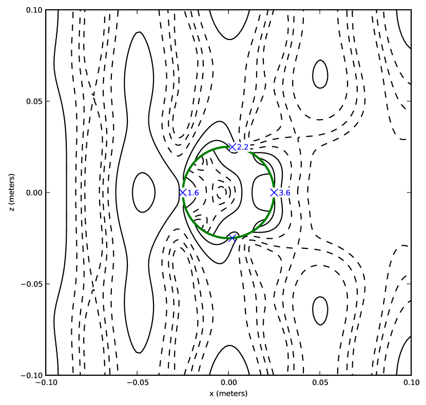
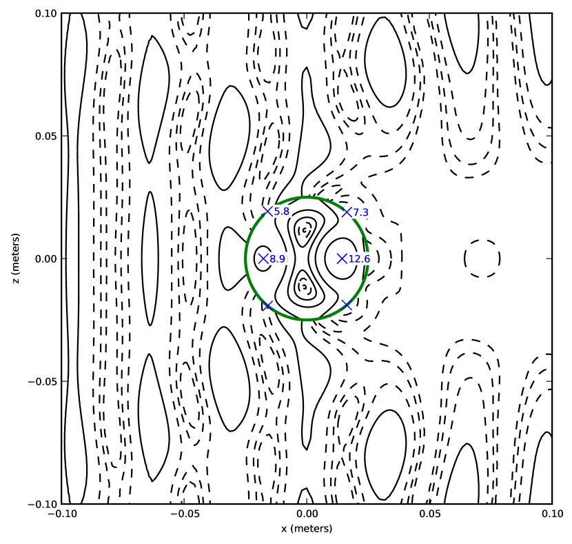
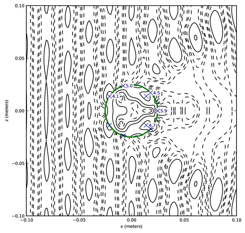
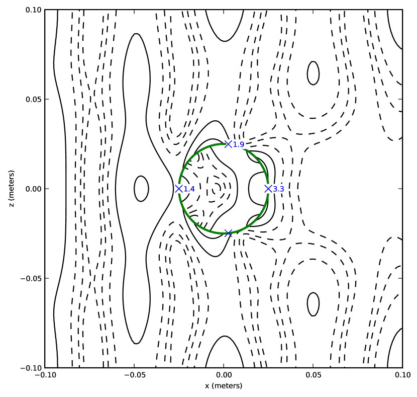
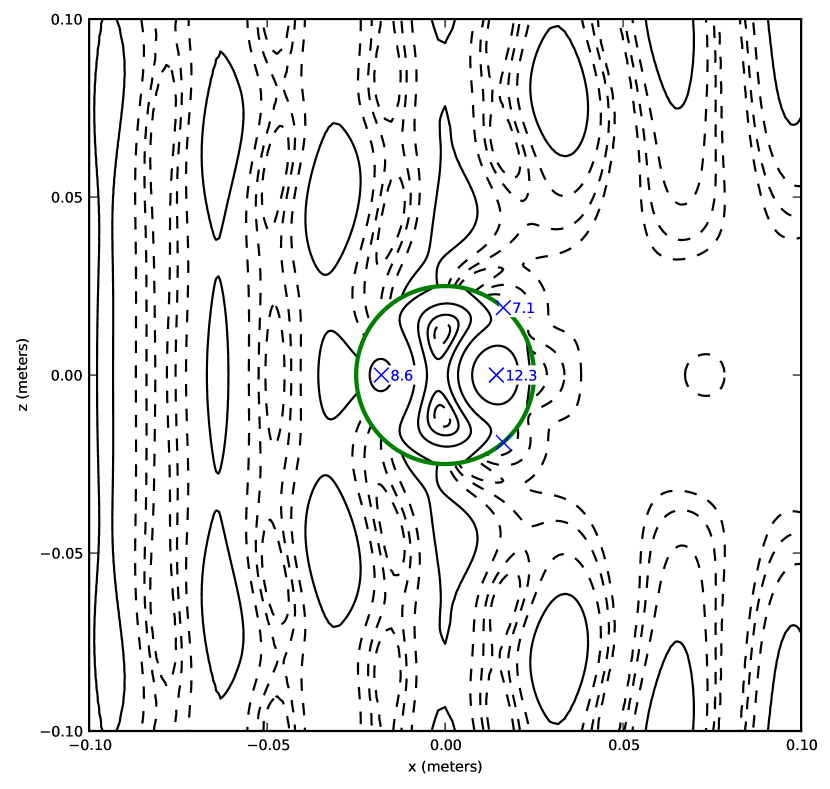
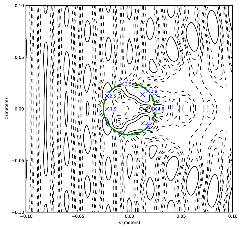
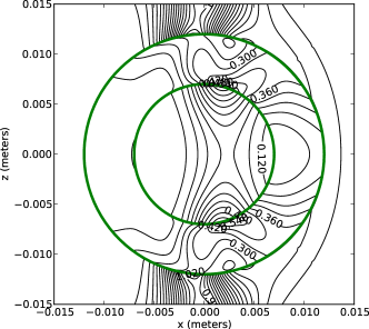
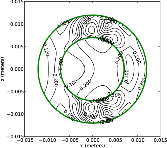
Figure 10 shows a few relevant quantities from this simulation, at a snapshot 18 $\mu$s after the start. We plot energy density normalized by the peak energy density of the incident pulse, for comparison with the cylindrical scatterer plots, as well as the maximum in-plane shear stress, as a general measure of the deformational load on the bone. We also plot some quantities that may be biologically relevant: the fluid pressure in the bone, and the magnitude of fluid flow velocity (the fluid volume flow rate $\mathbf{q}$ divided by porosity). The inclusion of the latter two is motivated by the review paper of Hillsley and Frangos [25], who identify interstitial fluid flow as relevant to osteogenesis. While the plots Figure 10 show some artifacts due to the highly distorted grid mapping — namely, the kinks in some of the contours along the lines of nearly triangular cells extending diagonally from the center of the circles — the solution looks qualitatively good overall. At the point shown in the solution, the leading fast P wavefront has passed entirely through the bone. Meanwhile, separate fast P and S waves from the initial impact of the pulse, visible in Figures 10a and 10b as the lobes coming off vertically and to the right from the top and bottom of the cancellous bone core, are still propagating through the cortical bone. There are local regions of high fluid velocity (Figure 10c), particularly in the cancellous bone but also associated with the fast P wave propagating around the cortical bone; there are also local regions of high or low fluid pressure, associated with a slow P wave to the left of the top and bottom of the cancellous core in Figure 10d, and with the reflection of the fast P wave off the right exterior surface of the cortical bone. The response of the pore fluids is hampered, though, by the impermeability of the bone surfaces, which prevents strong slow P waves from being excited by the incident wave.

(a) Normalized energy density

(b) Maximum in-plane shear stress (Pa)

(c) Fluid flow speed ($\mu$m/s)

(d) Pressure (Pa)

Fig. 10: Contour plots of various solution quantities in the femur model, 18 $\mu$s after the start of the simulation. The thick circles mark the boundaries between different media.

6 Summary and future work

We have developed a high-resolution finite volume method code to model wave propagation in two dimensions in systems of multiple orthotropic media and/or fluids. Our code is capable of using mapped grids to model curved interfaces, and can also model several standard interface conditions used for hydraulic contact with a poroelastic medium — specifically, open pores, sealed pores, or imperfect hydraulic contact. In order to correctly model interfaces between poroelastic materials and fluids, we have introduced a new transverse Riemann solution scheme that more carefully handles transverse updates to media goverened by different systems of equations. We have also found that in order to avoid having the poroelastic variables contaminate the solution in the fluid, at these interfaces we must omit the standard second-order correction term used in high-resolution finite volume methods. While it seems possible to generalize the second-order correction term to these cases, for now we accept the reduction in accuracy in the interface cells.

In order to verify our code, we examined its convergence for a variety of analytical solutions. We first investigated the effect of omitting the second-order correction term at an interface using simple plane wave solutions, by omitting the correction along a line through our computational domain. In the 1-norm we observed second-order convergence with error nearly as low as if the second-order term were present everywhere; in the max-norm, convergence was degraded to first-order, but the magnitude of the error was substantially lower than for a wholly first-order method. Following this, we tested the ability of our code to model interfaces between media by comparing its results to analytical solutions for a time-harmonic plane wave being reflected off and transmitted through a material interface — either between a fluid and a poroelastic medium or between two different poroelastic media. We achieved the convergence results that were to be expected from the plane wave tests: second-order convergence in 1-norm and first-order in the max-norm, demonstrating that our code can model wave reflection and transmission at an interface with reasonable accuracy.

Next, we evaluated the ability of our code to handle curved interfaces and mapped grids by applying it to a time-harmonic acoustic plane wave scattering off a poroelastic cylinder. Convergence results were substantially degraded, to not much better than first-order in the 1-norm, and to roughly order $\frac{1}{2}$ in the max-norm. The reason for this was the highly-distorted cells where the mapping function mapped the corners of a square in the computational domain to the surface of a circle in the physical domain. This type of problem is unavoidable when making a logically rectangular grid of this type, but these error results could be ameliorated somewhat in the future by aggressive use of adaptive mesh refinement at the problem cells; in any case, the numerical solution on a fine grid after one cycle closely matched the true solution. We also simulated a simplified model of a human femur bone in a water bath being struck by a pressure pulse; all three poroelastic waves contribute noticeably to the response of the bone, and localized regions of high stress, pressure, and fluid flow rate occur, which may be of interest biologically.

From here, there are several open directions for future work. The most obvious is development of a generalized second-order correction term that can be used at a material interface; an approach based on the Immersed Interface Method [35, 41, 42] seems effective, but formulating an appropriate limiting scheme for this case is not trivial. Another obvious extension is to three-dimensional models, in order to handle more interesting and realistic systems. The move to three dimensions is straightforward, but as always the increase in computational work from two dimensions to three is quite large. In particular, the number of transverse Riemann solves grows dramatically in three dimensions [31], which may necessitate use of dimensional splitting instead.

There are also opportunities for expansion of the frequency range in which our code is valid, and in which it achieves its optimal order of accuracy. While this paper has avoided the stiff regime identified in our previous work [33], it still represents an impediment to second-order convergence in cases where an otherwise reasonable grid and CFL number result in a timestep much longer than the characteristic dissipation time for the material; this might be alleviated by an improved Riemann solution process that takes into account the effect of the dissipation term on the evolution of the waves, possibly using the work of Hittinger and Roe [26] on Riemann solutions of hyperbolic systems with relaxation terms, or by using a semidiscrete numerical scheme with an exponential time-integrator [27] that more explicitly models the effect of the stiff relaxation term. Finally, while we model low-frequency Biot theory here, our code could be extended straightforwardly to higher-frequency poroelasticity models by the inclusion of additional memory variables to model the frequency-dependent kernel used for the generalization of Darcy’s law to high frequencies [36].

To aid in reproducibility, we provide all of the code used to generate the results here at
http://dx.doi.org/10.6084/m9.figshare.701483.

7 Acknowledgements

This work has benefited greatly from the direct input and advice of Prof. Randall J. LeVeque of the Department of Applied Mathematics, University of Washington, as well as from the clawpack simulation framework.

Appendix A Solution of the poroelastic eigenproblem

A.1 Equipartition of energy

A useful property that can be derived from the block structure of the system is that a simple plane wave of the homogeneous hyperbolic equation (3) carries equal amounts of kinetic and potential energy. To see this, note that a simple traveling plane wave solution has the form $\mbox{$\mathbf{Q}$}(x,z,t)=\mathbf{r}f(n_{x}x+n_{z}z-\lambda t)$, where $\mathbf{r}$ and $\lambda$ satisfy the eigenproblem

$$\breve{\mbox{$\mathbf{A}$}}\mathbf{r}=\lambda\mathbf{r},\quad\breve{\mbox{$\mathbf{A}$}}:=n_{x}\mbox{$\mathbf{A}$}+n_{z}\mbox{$\mathbf{B}$}.$$ (38)

For a traveling wave, we further assume $\lambda$ is nonzero. Dividing $\mathbf{r}$ into stress and velocity parts according to the block partitioning of the system, $\mathbf{r}=:\begin{pmatrix}\mathbf{r}_{s}^{T}&\mathbf{r}_{v}^{T}\end{pmatrix}^{T}$, this becomes a pair of equations,

$$\breve{\mbox{$\mathbf{A}$}}_{sv}\mathbf{r}_{v}=\lambda\mathbf{r}_{s},\quad\breve{\mbox{$\mathbf{A}$}}_{vs}\mathbf{r}_{s}=\lambda\mathbf{r}_{v},$$ (39)

or, multiplying through by $\mathbf{E}$,

$$\mbox{$\mathbf{E}$}_{s}\breve{\mbox{$\mathbf{A}$}}_{sv}\mathbf{r}_{v}=\lambda\mbox{$\mathbf{E}$}_{s}\mathbf{r}_{s},\quad\mbox{$\mathbf{E}$}_{v}\breve{\mbox{$\mathbf{A}$}}_{vs}\mathbf{r}_{s}=\lambda\mbox{$\mathbf{E}$}_{v}\mathbf{r}_{v}.$$ (40)

Now, multiply the first equation of (40) from the left by $\mathbf{r}_{s}^{T}$, giving

$$\mathbf{r}_{s}^{T}\mbox{$\mathbf{E}$}_{s}\breve{\mbox{$\mathbf{A}$}}_{sv}\mathbf{r}_{v}=\lambda\mathbf{r}_{s}^{T}\mbox{$\mathbf{E}$}_{s}\mathbf{r}_{s},$$ (41)

and notice the symmetry relation between blocks (due to $\mathbf{E}$$\mathbf{A}$ and $\mathbf{E}$$\mathbf{B}$ being symmetric as discussed in [33], and remaining symmetric when the state variable are permuted to the order used in this work),

$$\mbox{$\mathbf{E}$}_{s}\mbox{$\mathbf{A}$}_{sv}=(\mbox{$\mathbf{E}$}_{v}\mbox{$\mathbf{A}$}_{vs})^{T},\quad\mbox{$\mathbf{E}$}_{s}\mbox{$\mathbf{B}$}_{sv}=(\mbox{$\mathbf{E}$}_{v}\mbox{$\mathbf{B}$}_{vs})^{T}.$$ (42)

Using this symmetry relation and the eigenproblem (40), $\mathbf{r}_{s}^{T}\mbox{$\mathbf{E}$}_{s}\breve{\mbox{$\mathbf{A}$}}_{sv}=\mathbf{r}_{s}^{T}(\mbox{$\mathbf{E}$}_{v}\breve{\mbox{$\mathbf{A}$}}_{vs})^{T}=(\mbox{$\mathbf{E}$}_{v}\breve{\mbox{$\mathbf{A}$}}_{vs}\mathbf{r}_{s})^{T}=(\lambda\mbox{$\mathbf{E}$}_{v}\mathbf{r}_{v})^{T}$. Since we took $\lambda\neq 0$ for a traveling wave, we may divide it out; remembering that $\mbox{$\mathbf{E}$}_{v}$ is symmetric, we obtain

$$\mathbf{r}_{v}^{T}\mbox{$\mathbf{E}$}_{v}\mathbf{r}_{v}=\mathbf{r}_{s}^{T}\mbox{$\mathbf{E}$}_{s}\mathbf{r}_{s}.$$ (43)

Note that there is no need to distinguish between the ordinary transpose and the Hermitian here, since as demonstrated in [33] the eigenvectors are real-valued. Note also that there was no specific reference to the physics of poroelastic medium here, only to general algebraic properties of the system — it is easy to verify that the matrices for linear acoustics satisfy the same block symmetry relations, so the same $\mathbf{E}$-orthogonality and energy equipartition results hold for acoustics as well.

A.2 Solution of the eigenproblem

In order to solve the Riemann problem, we first need the eigenvalues and eigenvectors of the $\breve{\mbox{$\mathbf{A}$}}$ matrix on either side of the interface. For our poroelastic material of interest, let $(n_{1},n_{3})$ be the components of the unit normal to the Riemann solve interface, measured in the material principal coordinates. Then if we write the first-order system (2) in principal coordinates, $\breve{\mbox{$\mathbf{A}$}}$ is

$$\breve{\mbox{$\mathbf{A}$}}=n_{1}\mbox{$\mathbf{A}$}+n_{3}\mbox{$\mathbf{B}$},$$ (44)

where $\mathbf{A}$ and $\mathbf{B}$ are exactly as given in (4), (5), and (6). Furthermore, from the properties of $\mathbf{A}$ and $\mathbf{B}$, we know that $\mbox{$\mathbf{E}$}\breve{\mbox{$\mathbf{A}$}}$ is symmetric, and if we define $\breve{\mbox{$\mathbf{A}$}}_{sv}:=n_{1}\mbox{$\mathbf{A}$}_{sv}+n_{3}\mbox{$\mathbf{B}$}_{sv}$ and $\breve{\mbox{$\mathbf{A}$}}_{vs}:=n_{1}\mbox{$\mathbf{A}$}_{vs}+n_{3}\mbox{$\mathbf{B}$}_{vs}$, then $\mbox{$\mathbf{E}$}_{s}\breve{\mbox{$\mathbf{A}$}}_{sv}=(\mbox{$\mathbf{E}$}_{v}\breve{\mbox{$\mathbf{A}$}}_{vs})^{T}$.

In order to see how this helps us, let $\lambda$ and $\mathbf{r}$ be an eigenpair of $\breve{\mbox{$\mathbf{A}$}}$, so that $\breve{\mbox{$\mathbf{A}$}}\mathbf{r}=\lambda\mathbf{r}$. Since $\mathbf{E}$ is nonsingular, this is equivalent to the generalized eigenproblem

$$\mbox{$\mathbf{E}$}\breve{\mbox{$\mathbf{A}$}}\mathbf{r}=\lambda\mbox{$\mathbf{E}$}\mathbf{r}.$$ (45)

Dividing the eigenvector into stress and velocity blocks, $\mathbf{r}=:\begin{pmatrix}\mathbf{r}_{s}^{T}&\mathbf{r}_{v}^{T}\end{pmatrix}^{T}$, and referring back to section 2, we can rewrite the second equation of (40) as $(\mbox{$\mathbf{E}$}_{s}\breve{\mbox{$\mathbf{A}$}}_{sv})^{T}\mathbf{r}_{s}=\breve{\mbox{$\mathbf{A}$}}_{sv}^{T}\mbox{$\mathbf{E}$}_{s}\mathbf{r}_{s}=\lambda\mbox{$\mathbf{E}$}_{v}\mathbf{r}_{v}$. If we then multiply the first equation on the left by $\breve{\mbox{$\mathbf{A}$}}_{sv}^{T}$, we then get a $4\times 4$ symmetric-definite eigenproblem for $\lambda^{2}$ and $\mathbf{r}_{v}$:

$$\breve{\mbox{$\mathbf{A}$}}_{sv}^{T}\mbox{$\mathbf{E}$}_{s}\breve{\mbox{$\mathbf{A}$}}_{sv}\mathbf{r}_{v}=\lambda^{2}\mbox{$\mathbf{E}$}_{v}\mathbf{r}_{v}.$$ (46)

Aside from reducing the dimension of the eigenproblem, this also illustrates that the eigenvalues of this system come in positive and negative pairs – if $\lambda$ is an eigenvalue, then so is $-\lambda$.

While the reduction from an $8\times 8$ unsymmetric ordinary eigenproblem to a $4\times 4$ symmetric-definite generalized eigenproblem is already a substantial gain, further improvement is possible. First, factorize $\mbox{$\mathbf{E}$}_{v}$ as $\mbox{$\mathbf{E}$}_{v}=\mathbf{L}\mathbf{L}^{T}$, where $\mathbf{L}$ is upper-triangular; such an $\mathbf{L}$ can be found straightforwardly as

$$\mathbf{L}=\begin{pmatrix}\sqrt{\frac{\Delta_{1}}{m_{1}}}&0&\frac{\rho_{f}}{\sqrt{m_{1}}}&0\\ 0&\sqrt{\frac{\Delta_{3}}{m_{3}}}&0&\frac{\rho_{f}}{\sqrt{m_{3}}}\\ 0&0&\sqrt{m_{1}}&0\\ 0&0&0&\sqrt{m_{3}}\end{pmatrix}.$$ (47)

(We could choose many factorizations of $\mbox{$\mathbf{E}$}_{v}$, but the upper-triangular structure of $\mathbf{L}$ will be useful later. The $\Delta$ quantities are defined as $\Delta_{i}:=\rho m_{i}-\rho_{f}^{2}$.) Making the variable substitution $\mathbf{r}_{v}=\mathbf{L}^{-T}\mathbf{y}$, we arrive at the $4\times 4$ symmetric eigenproblem

$$\mathbf{M}_{4}\mathbf{y}=\lambda^{2}\mathbf{y},\quad\mathbf{M}_{4}:=\mathbf{L}^{-1}\breve{\mbox{$\mathbf{A}$}}_{sv}^{T}\mbox{$\mathbf{E}$}_{s}\breve{\mbox{$\mathbf{A}$}}_{sv}\mathbf{L}^{-T}.$$ (48)

As an aside, the way the matrix $\mathbf{M}_{4}$ is defined offers an additional opportunity to reduce the amount of computation performed during the Riemann solve. Substituting $\breve{\mbox{$\mathbf{A}$}}_{sv}=n_{1}\mbox{$\mathbf{A}$}_{sv}+n_{3}\mbox{$\mathbf{B}$}_{sv}$ into the definition of $\mathbf{M}_{4}$, we can reduce it to a quadratic form in $n_{1}$ and $n_{3}$ with matrix coefficients,

$$\mathbf{M}_{4}=n_{1}^{2}\mathbf{M}_{411}+n_{1}n_{3}\mathbf{M}_{413}+n_{3}^{2}\mathbf{M}_{433},$$ (49)

where

$$\mathbf{M}_{411} =\mathbf{L}^{-1}\mbox{$\mathbf{A}$}_{sv}^{T}\mbox{$\mathbf{E}$}_{s}\mbox{$\mathbf{A}$}_{sv}\mathbf{L}^{-T}$$ (50)

$$\mathbf{M}_{413} =\mathbf{L}^{-1}\mbox{$\mathbf{A}$}_{sv}^{T}\mbox{$\mathbf{E}$}_{s}\mbox{$\mathbf{B}$}_{sv}\mathbf{L}^{-T}+\mathbf{L}^{-1}\mbox{$\mathbf{B}$}_{sv}^{T}\mbox{$\mathbf{E}$}_{s}\mbox{$\mathbf{A}$}_{sv}\mathbf{L}^{-T}$$

$$\mathbf{M}_{433} =\mathbf{L}^{-1}\mbox{$\mathbf{B}$}_{sv}^{T}\mbox{$\mathbf{E}$}_{s}\mbox{$\mathbf{B}$}_{sv}\mathbf{L}^{-T}.$$

Since the matrices $\mathbf{M}_{411}$, $\mathbf{M}_{413}$, and $\mathbf{M}_{433}$ do not depend on the interface direction but only on the properties of the medium, they can be computed once for each material and retrieved when needed to form the full $\mathbf{M}_{4}$.

Finally, we can reduce the dimension of the eigenproblem even further by finding one of the eigenvectors explicitly and removing it from the computation. It is easy to verify that $\mathbf{r}_{v0}=\begin{pmatrix}0&0&-n_{3}&n_{1}\end{pmatrix}^{T}$ satisfies $\breve{\mbox{$\mathbf{A}$}}_{sv}\mathbf{r}_{v0}=0$; physically, $\mathbf{r}_{v0}$ corresponds to fluid flow parallel to the Riemann problem interface, which produces no propagating waves in invisicd Biot theory. This is in fact the only vector in the null space of $\breve{\mbox{$\mathbf{A}$}}_{sv}$, since the other three eigenvectors correspond to the three propagating waves with nonzero wave speeds $\lambda$. Thus $\mathbf{y}_{0}:=\mathbf{L}^{T}\mathbf{r}_{v0}/\|\mathbf{L}^{T}\mathbf{r}_{v0}\|_{2}$ is a null vector of $\mathbf{M}_{4}$. Now construct a $4\times 3$ matrix $\mathbf{Y}_{3}$ whose columns are orthonormal and all orthogonal to $\mathbf{y}_{0}$. (This is where the upper-triangular structure of $\mathbf{L}$ comes in handy, since it means that the first two components of $\mathbf{y}_{0}$ are zero, which makes this matrix easy to construct.) The matrix $\mathbf{Y}:=\begin{pmatrix}\mathbf{Y}_{3}&\mathbf{y}_{0}\end{pmatrix}$ is then an orthonormal matrix. Making the new variable substitution $\mathbf{y}=\mathbf{Y}\begin{pmatrix}\mathbf{u}^{T}&u_{0}\end{pmatrix}^{T}$ in (48) and multiplying from the left by $\mathbf{Y}^{T}$, we then get

$$\mathbf{Y}^{T}\mathbf{M}_{4}\mathbf{Y}\begin{pmatrix}\mathbf{u}\\ u_{0}\end{pmatrix}=\begin{pmatrix}\mathbf{Y}_{3}^{T}\mathbf{M}_{4}\mathbf{Y}_{3}&0\\ 0&0\end{pmatrix}\begin{pmatrix}\mathbf{u}\\ u_{0}\end{pmatrix}=\lambda^{2}\begin{pmatrix}\mathbf{u}\\ u_{0}\end{pmatrix}.$$ (51)

Since we are primarily concerned with propagating waves in the Riemann solution, we can ignore the possibility of $\lambda=0$, and need only find eigenvalues and eigenvectors of the $3\times 3$ matrix $\mathbf{M}_{3}:=\mathbf{Y}_{3}^{T}\mathbf{M}_{4}\mathbf{Y}_{3}$. We use the classic QR algorithm with Wilkinson shifts for this, following the implementation outlined in Golub and van Loan [23], which has the advantages of being fairly straightforward to implement and computing all the eigenvectors at once.

The QR algorithm also has another beneficial property for our Riemann solution process. It naturally produces eigenvectors with unit 2-norm, which is useful in the orthonormalization of the eigenvectors. Backing out the variable transformations above, we get $\mathbf{r}_{v}=\mathbf{L}^{-T}\mathbf{Y}_{3}\mathbf{u}$, so $\mathbf{r}_{v}^{T}\mbox{$\mathbf{E}$}_{v}\mathbf{r}_{v}=\mathbf{u}^{T}\mathbf{u}$. If we divide each eigenvector $\mathbf{u}$ by $\sqrt{2}$ after computing it with the QR algorithm, we get $\mathbf{r}_{v}^{T}\mbox{$\mathbf{E}$}_{v}\mathbf{r}_{v}=\frac{1}{2}$, and by the energy equipartition result (43), $\mathbf{r}^{T}\mbox{$\mathbf{E}$}\mathbf{r}=\mathbf{r}_{s}^{T}\mbox{$\mathbf{E}$}_{s}\mathbf{r}_{s}+\mathbf{r}_{v}^{T}\mbox{$\mathbf{E}$}_{v}\mathbf{r}_{v}=2\mathbf{r}_{v}^{T}\mbox{$\mathbf{E}$}_{v}\mathbf{r}_{v}=1$. This energy orthonormalization is helpful for calculating wave strengths in the common special case of a Riemann problem between identical poroelastic materials.

Once we have $\lambda^{2}$ and $\mathbf{r}_{v}$, we get $\lambda$ as either the positive or negative square root of $\lambda^{2}$; negative $\lambda$ values correspond to left-going waves, while positive $\lambda$ indicate right-going waves. Since we have excluded the null space of $\breve{\mbox{$\mathbf{A}$}}_{sv}$ when calculating these eigensolutions, no $\lambda$ thus obtained will be zero. Finally, we can use (39) to obtain $\mathbf{r}_{s}=\breve{\mbox{$\mathbf{A}$}}_{sv}\mathbf{r}_{v}/\lambda$, giving all the components of the eigenvector $\mathbf{r}$ measured in the principal axes of the material; we then transform $\mathbf{r}$ into the global computational axes to solve the Riemann problem.

Appendix B Analytic solution procedure for a time-harmonic plane wave train striking a flat interface

To obtain an analytic solution for a sinusoidal plane wave train striking a planar interface between two poroelastic media, or a poroelastic medium and a fluid, we first specify the angular frequency $\omega$ of the solution, the unit vector $\mathbf{p}$ in the propagation direction of the incident wave, and the wave family desired if the incident wave is in a poroelastic medium. Calculations will be done with a complex-valued solution for convenience; for actual use, we take the real part of this solution.

We assume an ansatz for the incident wave of the form

$$\mbox{$\mathbf{Q}$}_{\text{in}}(\mathbf{x},t)=\mathbf{V}_{\text{in}}\exp\left(i(k_{\text{in}}\mathbf{x}\cdot\mathbf{p}-\omega t)\right),$$ (52)

Substuting this into the PDE (2), which models both poroelasticity and acoustics depending on the choice of coefficient matrices, we obtain the eigenvalue problem

$$-i\omega\mathbf{V}_{\text{in}}+ik_{\text{in}}(p_{x}\mbox{$\mathbf{A}$}_{R}+p_{z}\mbox{$\mathbf{B}$}_{R})\mathbf{V}_{\text{in}}=\mbox{$\mathbf{D}$}_{R}\mathbf{V}_{\text{in}}.$$ (53)

Note that here $\mbox{$\mathbf{A}$}_{R}$ and $\mbox{$\mathbf{B}$}_{R}$ are taken to be in the global $x$-$z$ axes, rather than the material principal axes. The subscript $R$ denotes the side of the interface corresponding to the incident and reflected waves, as opposed to $T$, which will denote the side corresponding to the transmitted waves. We solve this eigenproblem for $k_{\text{in}}$ and $\mathbf{V}_{\text{in}}$, and select the appropriate solution for the desired wave family, if applicable. We typically scale the eigenvector $\mathbf{V}_{\text{in}}$ to have unit energy norm.

With the incident wave solution in hand, we turn to the reflected and transmitted waves. We expect a reflected or transmitted wave in every wave family in each medium, although some of these may be evanescent waves if the angle of incidence is shallow enough. While evanescent waves decay rapidly away from the interface, they are important near it and must be included in the solution if they occur. We assume that each reflected and transmitted wave has a similar complex exponential form to the incoming wave, but with wavevectors whose magnitude and direction are both unknown. Specifically, we take the ansatz

$$\mbox{$\mathbf{Q}$}_{(R,T)j}(\mathbf{x},t)=\mathbf{V}_{(R,T)j}\exp\left(i(\mathbf{k}_{(R,T)j}\cdot\mathbf{x}-\omega t)\right),$$ (54)

where $j$ indexes the wave family and $(R,T)$ may be either $R$ or $T$ — this equation holds for both the reflected and the transmitted waves. We then take the total solution field $\mbox{$\mathbf{Q}$}(\mathbf{x},t)$ to be

$$\mbox{$\mathbf{Q}$}(\mathbf{x},t)=\begin{cases}\mbox{$\mathbf{Q}$}_{\text{in}}(\mathbf{x},t)+\sum_{j=1}^{N_{R}}\mbox{$\mathbf{Q}$}_{Rj}(\mathbf{x},t),\quad&\text{$\mathbf{x}$ on incident side of interface,}\\ \sum_{j=1}^{N_{T}}\mbox{$\mathbf{Q}$}_{Tj}(\mathbf{x},t),\quad&\text{$\mathbf{x}$ on outgoing side of interface,}\end{cases}$$ (55)

where $N_{R}$ and $N_{T}$ are the numbers of reflected and transmitted waves.

At first glance, there seem to be too many unknowns to find a unique solution for each wave, but it is also necessary to satisfy the appropriate interface condition; denoting the incident and outgoing sides of the interface by the subscripts “in” and “out,” this condition becomes $\mathbf{C}_{\text{in}}\mbox{$\mathbf{Q}$}_{\text{in, total}}=\mathbf{C}_{\text{out}}\mbox{$\mathbf{Q}$}_{\text{out}}$, where $\mbox{$\mathbf{Q}$}_{\text{in, total}}$ and $\mbox{$\mathbf{Q}$}_{\text{out}}$ are the limits of the state vector approaching the interface from the incoming and outgoing sides, and $\mathbf{C}_{\text{in}}$ and $\mathbf{C}_{\text{out}}$ are the interface condition matrices of section 3.2.3. Writing $\mbox{$\mathbf{Q}$}_{\text{in, total}}$ and $\mbox{$\mathbf{Q}$}_{\text{out}}$ in terms of individual waves, we get

$$\mathbf{C}_{\text{in}}\left.\left(\mbox{$\mathbf{Q}$}_{\text{in}}(\mathbf{x},t)+\sum_{j=1}^{N_{R}}\mbox{$\mathbf{Q}$}_{Rj}(\mathbf{x},t)\right)\right|_{\text{at interface}}=\mathbf{C}_{\text{out}}\left.\sum_{j=1}^{N_{T}}\mbox{$\mathbf{Q}$}_{Tj}(\mathbf{x},t)\right|_{\text{at interface}}.$$ (56)

Now, let $\mathbf{t}$ be the unit tangent vector along the interface; without loss of generality assume that the interface runs through the origin of coordinates, and let $\xi$ measure distance along it from the origin. Factoring out the $\exp(-i\omega t)$ time dependence, the interface condition (56) becomes

$$\mathbf{C}_{\text{in}}\left(\mathbf{V}_{\text{in}}\exp(ik_{\text{in}}\mathbf{p}\cdot\mathbf{t}\,\xi)+\sum_{j=1}^{N_{R}}\mathbf{V}_{Rj}\exp(i\mathbf{k}_{Rj}\cdot\mathbf{t}\,\xi)\right)=\mathbf{C}_{\text{out}}\sum_{j=1}^{N_{T}}\mathbf{V}_{Tj}\exp(i\mathbf{k}_{Tj}\cdot\mathbf{t}\,\xi).$$ (57)

For this condition to hold at all points on the interface, it is necessary to have $\mathbf{k}_{(R,T)j}\cdot\mathbf{t}=k_{\text{in}}\mathbf{p}\cdot\mathbf{t}$ for every reflected and transmitted wave; we denote this common tangential component of the wavevector as $k_{t}$, and note that it is entirely specified by the direction and frequency of the incident wave.

Expressing (2) in coordinates tangential and normal to the interface, then applying it to the ansatz (54) and dividing out the exponential time and space depedence, we obtain for each outgoing wave

$$-i\omega\mathbf{V}_{(R,T)j}+ik_{t}\breve{\mbox{$\mathbf{A}$}}_{(R,T)}\mathbf{V}_{(R,T)j}+ik_{(R,T)nj}\breve{\mbox{$\mathbf{B}$}}_{(R,T)}\mathbf{V}_{(R,T)j}=\mbox{$\mathbf{D}$}_{(R,T)}\mathbf{V}_{(R,T)j}.$$ (58)

Here $\breve{\mbox{$\mathbf{A}$}}_{(R,T)}=t_{x}\mbox{$\mathbf{A}$}_{(R,T)}+t_{z}\mbox{$\mathbf{B}$}_{(R,T)}$ is the flux Jacobian in the tangential direction, and $\breve{\mbox{$\mathbf{B}$}}_{(R,T)}=-t_{z}\mbox{$\mathbf{A}$}_{(R,T)}+t_{x}\mbox{$\mathbf{B}$}_{(R,T)}$ is the flux Jacobian in the direction normal to the interface; $k_{(R,T)nj}$ is the component of the wavevector in the interface normal direction. The subscript $(R,T)$ is included as a reminder that the system matrices will in general be different on either side of the interface. Multiplying from the left by $\mbox{$\mathbf{E}$}_{(R,T)}$ to symmetrize and reorganizing, we obtain a complex symmetric generalized eigenproblem for each $k_{(R,T)nj}$ and its corresponding $\mathbf{V}_{(R,T)j}$:

$$\left(\omega\mbox{$\mathbf{E}$}_{(R,T)}-k_{t}\mbox{$\mathbf{E}$}_{(R,T)}\breve{\mbox{$\mathbf{A}$}}_{(R,T)}-i\mbox{$\mathbf{E}$}_{(R,T)}\mbox{$\mathbf{D}$}_{(R,T)}\right)\mathbf{V}_{(R,T)j}=k_{(R,T)nj}\mbox{$\mathbf{E}$}_{(R,T)}\breve{\mbox{$\mathbf{B}$}}_{(R,T)}\mathbf{V}_{(R,T)j}.$$ (59)

Because these represent reflected and transmitted waves, we choose the eigenvalues $k_{(R,T)nj}$ that correspond to waves propagating away from the interface (for pure real eigenvalues, for which we determine propagation direction from the sign of the normal energy flux $\mbox{$\mathbf{Q}$}^{H}\mbox{$\mathbf{E}$}\breve{\mbox{$\mathbf{B}$}}\mbox{$\mathbf{Q}$}$), or that decay away from the interface (for complex eigenvalues). As a practical note, $\breve{\mbox{$\mathbf{B}$}}$ is always singular, and for our formulation of acoustics the matrix on the left-hand side is also singular with some of its null space in common with $\breve{\mbox{$\mathbf{B}$}}$, so this eigenproblem presents numerical difficulties (see, for example, section 7.7.3 of Golub and van Loan [23]). To obtain an accurate solution, we found it necessary to make an additional change of variables to eliminate the null spaces of both matrices, then solve a smaller generalized eigenproblem with both matrices nonsingular. For the actual eigensolution, we used the eig command in Scipy [30], which in turn calls the LAPACK [1] routine ZGGEV.

Combined with $k_{t}$, these eigensolutions fully define the reflected and transmitted waves of (54) up to a scalar factor; because we have not yet determined that factor, we denote the eigenvectors found from (59) by $\mathbf{v}_{(R,T)j}$, and let $\mathbf{V}_{(R,T)j}=\beta_{(R,T)j}\mathbf{v}_{(R,T)j}$. To find these scalar factors, we return to (57) and divide out the common factor of $\exp(ik_{t}\xi)$ to obtain

$$\mathbf{C}_{\text{in}}\left(\mathbf{V}_{\text{in}}+\sum_{j=1}^{N_{R}}\beta_{Rj}\mathbf{v}_{Rj}\right)=\mathbf{C}_{\text{out}}\sum_{j=1}^{N_{T}}\beta_{Tj}\mathbf{v}_{Tj}.$$ (60)

Rearranging and casting in matrix form, we obtain a linear system for the $\beta$ values,

$$\begin{pmatrix}-\mathbf{C}_{\text{in}}\mathbf{v}_{R1}&\dots&-\mathbf{C}_{\text{in}}\mathbf{v}_{RN_{R}}&\mathbf{C}_{\text{out}}\mathbf{v}_{T1}&\dots&\mathbf{C}_{\text{out}}\mathbf{v}_{TN_{T}}\end{pmatrix}\begin{pmatrix}\beta_{R1}\\ \vdots\\ \beta_{RN_{R}}\\ \beta_{T1}\\ \vdots\\ \beta_{TN_{T}}\end{pmatrix}=\mathbf{C}_{\text{in}}\mathbf{V}_{\text{in}}.$$ (61)

Solving this system completes the information necessary to describe the reflected and transmitted wave fields, and allows us to compute the full solution field at any point and time.

Appendix C Gallery of energy density plots for cylindrical scatterer cases

This section contains plots of the energy densities at the initial time for all 18 cases selected for convergence investigation in Section 5 of the main paper. The plots here also include locations and values of maxima of the energy density within the scatterer, which were omitted from the main paper due to the difficulty of including them legibly in a small plot. The plotting is the same as in Figure 8 of the main paper: the plotted quantity is the energy density, normalized by the peak energy density of the incident wave, and contours are placed at powers of 2, with dashed contours indicating negative powers and solid indicating positive powers. The blue $\times$ symbols indicate the locations of maxima, with the adjacent labels giving the value at those maxima. Since the solutions are symmetric top-to-bottom, only the top or bottom maximum of a pair is labeled, not both.

Fig. 11: Inviscid, $\eta_{d}=0$, 13.25 kHz

Fig. 12: Inviscid, $\eta_{d}=0$, 22.25 kHz

Fig. 13: Inviscid, $\eta_{d}=0$, 38.20 kHz

Fig. 14: Inviscid, $\eta_{d}=0.5$, 17.25 kHz

Fig. 15: Inviscid, $\eta_{d}=0.5$, 25.02 kHz

Fig. 16: Inviscid, $\eta_{d}=0.5$, 39.03 kHz

Fig. 17: Inviscid, $\eta_{d}=1$, 17.30 kHz

Fig. 18: Inviscid, $\eta_{d}=1$, 25.09 kHz

Fig. 19: Inviscid, $\eta_{d}=1$, 39.04 kHz

Fig. 20: Viscous, $\eta_{d}=0$, 15.70 kHz

Fig. 21: Viscous, $\eta_{d}=0$, 24.55 kHz

Fig. 22: Viscous, $\eta_{d}=0$, 38.39 kHz

Fig. 23: Viscous, $\eta_{d}=0.5$, 15.80 kHz

Fig. 24: Viscous, $\eta_{d}=0.5$, 24.54 kHz

Fig. 25: Viscous, $\eta_{d}=0.5$, 38.35 kHz

Fig. 26: Viscous, $\eta_{d}=1$, 15.80 kHz

Fig. 27: Viscous, $\eta_{d}=1$, 24.54 kHz

Fig. 28: Viscous, $\eta_{d}=1$, 38.35 kHz

References

- [1] E. Anderson, Z. Bai, C. Bischof, S. Blackford, J. Demmel, J. Dongarra, J. Du Croz, A. Greenbaum, S. Hammarling, A. McKenney, and D. Sorensen, LAPACK Users’ Guide, Society for Industrial and Applied Mathematics, Philadelphia, PA, third ed., 1999.
- [2] M. J. Berger and R. J. LeVeque, Adaptive mesh refinement using wave-propagation algorithms for hyperbolic systems, SIAM Journal on Numerical Analysis, 35 (1998), pp. 2298–2316.
- [3] M. A. Biot, Theory of propagation of elastic waves in a fluid-saturated porous solid. I. Low-frequency range, Journal of the Acoustical Society of America, 28 (1956), pp. 168–178.
- [4] , Theory of propagation of elastic waves in a fluid-saturated porous solid. II. Higher frequency range, Journal of the Acoustical Society of America, 28 (1956), pp. 179–191.
- [5] , Mechanics of deformation and acoustic propagation in porous media, Journal of Applied Physics, 33 (1962), pp. 1482–1498.
- [6] T. Bourbié, O. Coussy, and B. Zinszner, Acoustics of Porous Media, Gulf Publishing Company, Houston, Texas, 1987.
- [7] J. L. Buchanan, R. P. Gilbert, A. Wirgin, and Y. S. Xu, Marine acoustics: direct and inverse problems, SIAM, Philadelphia, 2004.
- [8] D. A. Calhoun, C. Helzel, and R. J. LeVeque, Logically rectangular finite volume grids and methods for circular and spherical domains, SIAM Review, 50 (2008), pp. 723–752.
- [9] J. M. Carcione, Wave Fields in Real Media: Wave Propagation in Anisotropic, Anelastic, and Porous Media, Elsevier, Oxford, 2001.
- [10] J. M. Carcione, C. Morency, and J. E. Santos, Computational poroelasticity – a review, Geophysics, 75 (2010), pp. 75A229–75A243.
- [11] G. Chiavassa and B. Lombard, Time domain numerical modeling of wave propagation in 2D acoustic / porous media, arXiv preprint arXiv:1109.3281, (2011).
- [12] G. Chiavassa and B. Lombard, Time domain numerical modeling of wave propagation in 2D heterogeneous porous media, Journal of Computational Physics, 230 (2011), pp. 5288–5309.
- [13] S. C. Cowin, Bone poroelasticity, Journal of Biomechanics, 32 (1999), pp. 217–238.
- [14] S. C. Cowin and L. Cardoso, Fabric dependence of bone ultrasound, Acta of Bioengineering and Biomechanics, 12 (2010).
- [15] S. C. Cowin and M. M. Mehrabadi, Identification of the elastic symmetry of bone and other materials, Journal of Biomechanics, 22 (1989), pp. 503–515.
- [16] J. de la Puente, M. Dumbser, M. Käser, and H. Igel, Discontinuous Galerkin methods for wave propagation in poroelastic media, Geophysics, 73 (2008), pp. T77–T97.
- [17] H. Deresiewicz and R. Skalak, On uniqueness in dynamic poroelasticity, Bulletin of the Seismological Society of America, 53 (1963), pp. 783–788.
- [18] S. Feng and D. L. Johnson, High-frequency acoustic properties of a fluid/porous solid interface. I. New surface mode, Journal of the Acoustical Society of America, 74 (1983), pp. 906–914.
- [19] R. F. Gibson, Principles of Composite Material Mechanics, McGraw-Hill, New York, 1994.
- [20] R. P. Gilbert, P. Guyenne, and M. Y. Ou, A quantitative ultrasound model of the bone with blood as the interstitial fluid, Mathematical and Computer Modelling, 55 (2012), pp. 2029–2039.
- [21] R. P. Gilbert and Z. Lin, Acoustic field in a shallow, stratified ocean with a poro-elastic seabed, Zeitschrift für Angewandte Mathematik und Mechanik, 77 (1997), pp. 677–688.
- [22] R. P. Gilbert and M. Y. Ou, Acoustic wave propagation in a composite of two different poroelastic materials with a very rough periodic interface: a homogenization approach, International Journal for Multiscale Computational Engineering, 1 (2003), pp. 157–163.
- [23] G. H. Golub and C. F. van Loan, Matrix Computations, Johns Hopkins University Press, Baltimore, third ed., 1996.
- [24] B. Gurevich and M. Schoenberg, Interface conditions for Biot’s equations of poroelasticity, Journal of the Acoustical Society of America, 105 (1999), pp. 2585–2589.
- [25] M. V. Hillsley and J. A. Frangos, Review: Bone tissue engineering: The role of interstitial fluid flow, Biotechnology and Bioengineering, 43 (1994), pp. 573–581.
- [26] J. A. F. Hittinger and P. L. Roe, Asymptotic analysis of the Riemann problem for constant coefficient hyperbolic systems with relaxation, Zeitschrift für Angewandte Mathematik und Mechanik, 84 (2004), pp. 452–471.
- [27] M. Hochbruck and A. Ostermann, Exponential integrators, Acta Numerica, 19 (2010), pp. 209–286.
- [28] A. Hosokawa and T. Otani, Ultrasonic wave propagation in bovine cancellous bone, Journal of the Acoustical Society of America, 101 (1997), pp. 558–562.
- [29] E. R. Hughes, T. G. Leighton, and P. R. White, Investigation of an anisotropic tortuosity in a biot model ultrasonic propagation in cancellous bone, Journal of the Acoustical Society of America, 121 (2007), pp. 568–574.
- [30] E. Jones, T. Oliphant, P. Peterson, et al., SciPy: Open source scientific tools for Python, 2001–.
- [31] J. O. Langseth and R. J. LeVeque, A wave propagation method for three-dimensional hyperbolic conservation laws, Journal of Computational Physics, 165 (2000), pp. 126–166.
- [32] J. Laperre and W. Thys, Scattering of ultrasonic waves by an immersed porous cylinder, Acoustics Letters, 16 (1992), pp. 9–16.
- [33] G. I. Lemoine, M. Y. Ou, and R. J. LeVeque, High-resolution finite volume modeling of wave propagation in orthotropic poroelastic media, SIAM Journal on Scientific Computing, 35 (2013), pp. B176–B206.
- [34] R. J. LeVeque, Finite Volume Methods for Hyperbolic Problems, Cambridge University Press, New York, 2002.
- [35] Z. Li and K. Ito, The immersed interface method: Numerical solutions of PDEs involving interfaces and irregular domains, Society for Industrial and Applied Mathematics, Philadelphia, Pennsylvania, 2006.
- [36] J.-F. Lu and A. Hanyga, Wave field simulation for heterogeneous porous media with singular memory drag force, Journal of Computational Physics, 208 (2005), pp. 651–674.
- [37] J. H. Rosenbaum, Synthetic microseismograms: logging in porous formations, Geophysics, 39 (1974), pp. 14–32.
- [38] M. D. Sharma, Wave propagation across the boundary between two dissimilar poroelastic solids, Journal of Sound and Vibration, 314 (2008), pp. 657–671.
- [39] T. H. Smit, J. M. Huyghe, and S. C. Cowin, Estimation of the poroelastic parameters of cortical bone, Journal of Biomechanics, 35 (2002), pp. 829–835.
- [40] The clawpack authors, clawpack software. www.clawpack.org.
- [41] C. Zhang, The immersed interface method for elastic wave propagations in heterogeneous materials. Rice University Department of Computational and Applied Mathematics Report TR96-29, 1996.
- [42] C. Zhang and R. J. LeVeque, Immersed interface methods for wave equations with discontinuous coefficients, Wave Motion, 25 (1997), pp. 237–263.