Phase Transition and Thermal Order-by-Disorder in the Pyrochlore Quantum Antiferromagnet Er2Ti2O7: A High-Temperature Series Expansion Study
Abstract
Several rare earth magnetic pyrochlore materials are well modeled by a spin- quantum Hamiltonian with anisotropic exchange parameters . For the Er2Ti2O7 material, the were recently determined from high-field inelastic neutron scattering measurements. Here, we perform high-temperature () series expansions to compute the thermodynamic properties of this material using these . Comparison with experimental data show that the model describes the material very well including the finite temperature phase transition to an ordered phase at K. We show that high temperature expansions give identical results for different order parameter susceptibilities up to order in (presumably to all orders in ). Conversely, a non-linear susceptibility related to the power of the order parameter reveals a thermal order-by-disorder selection of the same non-colinear “ state” as found in Er2Ti2O7.
pacs:
74.70.-b,75.10.Jm,75.40.Gb,75.30.DsOrder-by-disorder (ObD) is a beautiful concept of central importance in the field of frustrated magnetism. Villain ; Shender Saddled with large accidental degeneracies, a subset of states, those that support the largest quantum and/or thermal fluctuations, may be selected to form true long-range order, thus turning on its head the conventional wisdom of “less fluctuations lead to more order”. While ObD has been discussed theoretically for over thirty years, and proposed to be at play in a number of experimental settings, most recently in cold atom systems, ObD_cold_atoms convincing demonstrations of ObD in real materials have remained scarce. Yildirim ; Savary The main reason for the paucity of confirmed ObD material examplars is that the classical degeneracies are typically not sufficiently symmetry-protected to rule out that some weak energetic perturbations are responsible for stabilizing the observed long-range order. An exception is the long-range order found in the pyrochlore antiferromagnet Er2Ti2O7. Champion_PRB ; Ruff_ETO_PRL ; Poole Two groups Savary ; Zhitomirsky have recently put forward a strong case for a robust highly protected classical degeneracy in that system, hence making the case for ObD much more compelling than in any previous examples.
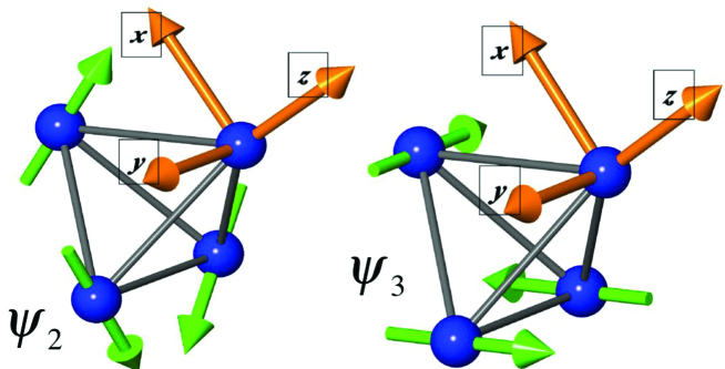
In an pyrochlore such as Er2Ti2O7, the ordered moments lie on average in an plane perpendicular to their local cubic direction. At the classical level, energetics further require a vanishing net magnetic moment on each elementary tetrahedron of the pyrochlore lattice. Particularly interesting is the fact that among all classically degenerate ground states that satisfy such zero tetrahedral moment configuration, the material orders at a critical temperature K in a ground state that breaks a discrete symmetry within the local plane – the so-called basis state of the irreducible representation (see Fig. 1). Champion_PRB ; Poole Since the original determination Champion_PRB of the long-range order in Er2Ti2O7, two rather puzzling questions had been identified: Firstly, how could the system order into a state that does not minimize the dipolar interactions, the so-called Palmer-Chalker state Palmer_Chalker which has each spin in its local plane? Secondly, what mechanism may lead to the selection, as opposed to the other basis vector of the two-dimensional manifold (see Fig.1), or even an arbitrary superposition of and arising from a spontaneous () global symmetry breaking?
Earlier studies had shown thermal Champion_PRB ; Champion_JPCM ; Stasiak and quantum Stasiak ObD selecting a state in a simplified pyrochlore antiferromagnetic model. More recent work found that anisotropic exchange can efficiently compete with dipolar interactions and lower the energy of below that of the Palmer-Chalker state. McClarty_ETO Building on these results, Savary et al. Savary showed that the classical degeneracies within are in fact immune to anisotropic bilinear spin-spin interactions of arbitrary form and range, leaving quantum ObD (q-ObD) as essentially but_VCFE the only plausible mechanism explaining the low-temperature state in Er2Ti2O7. A similar conclusion was reached in Ref. [Zhitomirsky, ]. The possible occurence of ObD in Er2Ti2O7 represents a potentially significant result in the field of highly frustrated magnetism.
While the arguments of Ref. Savary as per the symmetry-protection of degeneracy are compelling, there is still reason to worry whether the ordering mechanism in Er2Ti2O7 has indeed been fully unveiled. In particular, one may ask whether the model of Ref. Savary describes accurately the thermodynamic behavior of Er2Ti2O7 close to the transition and predict a K in accord with experiment. For example, since this was not investigated in Ref. Savary , a concern one might have is whether the model, for ignoring the long-range part of the dipole-dipole interactions dipoles_in_nn and other perturbations, does display a thermal ObD at in the correct state, rather than , which would then be inconsistent with experiments. double_transition Conversely, one may ask whether the experimentally observed state at low is the true ground state of the material or a metastable relic of the thermal ObD at . supp_mater Finally, the recent observation that there exists a tendency for rare-earth ions (e.g. R=Er3+ ) in R2Ti2O7 pyrochlore oxides to occupy the Ti4+ site at the 1% level, Ross_stuff hence generating effective random magnetic interactions, also raises concerns whether a plausible q-ObD at low temperatures smoothly merges to its thermal variant at .
The concerns above can only be alleviated by directly addressing, as we do in this paper, whether the model of Ref. [Savary, ] describes well the thermodynamic behavior of Er2Ti2O7 above . To do so, we use high-temperature expansions (HTE) and crystal-field theory to study the magnetic specific heat and susceptibility of the model. We also calculate order-parameter susceptibilities for and , finding that the model displays a continuous phase transition at a K close to the experimental value. By calculating a non-linear susceptibility, we show that order is indeed selected by thermal ObD. These results imply that the long-range part of the dipolar interactions neglected in Ref. [Savary, ] are not important above dipoles_in_nn and that the model of Ref. [Savary, ] is quantitatively accurate. We are thus rather confident that ObD, both thermal and quantum, cooperate in Er2Ti2O7 to select over the whole temperature range .
Model & method In a number of pyrochlore oxides Gardner , the single-ion crystal-field magnetic doublet ground state is separated from the lowest excited crystal-field energy levels by an energy gap that is large compared to the microscopic interactions, , between the ions. This is the case for Er2Ti2O7 for which K while K. In such a case, one can use an effective spin- Hamiltonian with bilinear anisotropic couplings, , to describe the interactions between ions, and where is the projection of onto the Hilbert space spanned by the single-ion ground doublets. On symmetry grounds, the nearest-neighbor can be parametrized by four exchange parameters as follows:
| (1) |
Here, refers to nearest-neighbor sites of the pyrochlore lattice, is a complex unimodular matrix, and Savary ; Ross . The quantization axis is along the local direction, and refers to the two orthogonal local directions. The were determined from fits to inelastic neutron scattering spectra in the field polarized state. Savary ; Js_values The magnetic properties of the system are described by the Zeeman Hamiltonian, added to , where is the angular momentum operator of Er3+, is the applied magnetic field, is the Bohr magneton and is the Er3+ Landé factor. Hz_form In this paper we investigate the thermodynamic properties of above and near using HTE. Series_book
We have computed series for the following quantities: (1) log of the partition function, , from which heat capacity and entropy are readily calculated; (2) uniform susceptibility as a linear response to a static applied external magnetic field; (3) linear order parameter susceptibilities, and , corresponding to and order, respectively; and (4) non-linear (4th and 6th order) order parameter cumulants associated with and long-range order. We discuss below the reason for calculating non-linear susceptibilities from these cumulants. supp_mater
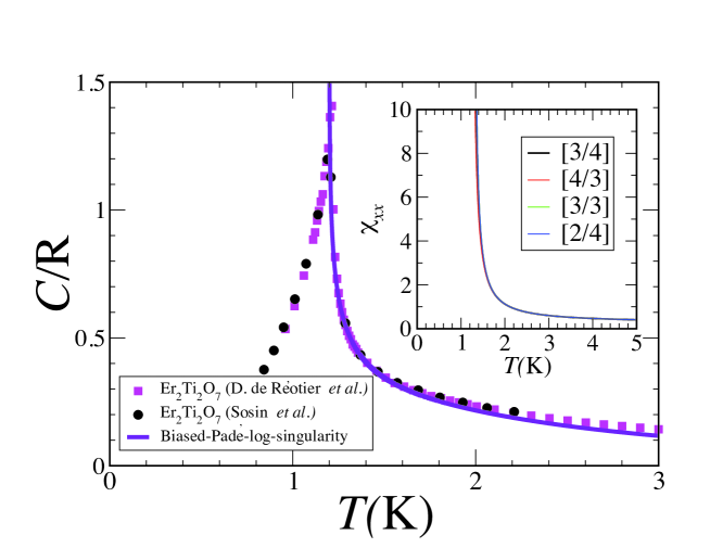
Demonstrating the validity of We first show evidence that the Hamiltonian (1) is consistent with a phase transition to long-range order in the components of the spins at a critical temperature K. To do so, we calculate high temperature series expansions for the order-parameter susceptibilities. We apply a field along the local ()-axis at all sites, and calculate the linear response order-parameter susceptibility, (). Detailed expressions can be found in the supplementary material supp_mater . As discussed in Refs. Savary ; Zhitomirsky , there is an emergent continuous symmetry in the model (1), which is only weakly lifted by higher order effects beyond classical ground state energetics. In the notation of Ref. Savary , this classical degeneracy can be parameterized by a continuous angle . Then, is the susceptibility for order (i.e. order) while is the susceptibility for order (i.e. order). We find that the two linear susceptibilities have identical high temperature series expansions to the order calculated (8th order in ). We believe that this result is true to all orders and the selection of order within the manifold must therefore only be manifest in non-linear order parameter susceptibilities. We return to this matter later. We study the singularities of the order-parameter susceptibility using d-log Padé approximants. Series_book Various estimated and critical exponents from near diagonal d-log Padé values, expressed in the form of ) sets, are , , and where is in Kelvin. Although the convergence is not excellent for this short series, we nevertheless conclude that the transition temperature is K. Given the large uncertainty in we cannot make a reliable estimate for , but its value is consistent with values known for -dimensional spin models. A plot of the order parameter susceptibility () versus temperature is shown in the inset of Fig. 2.
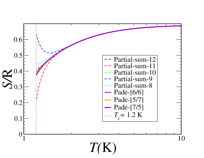
Next, we turn to a calculation of the specific heat, , and its comparison with experiments. We have calculated specific heat using both Numerical Linked Cluster (NLC) method Rigol ; Applegate ; Hayre and HTE. The two methods agree well at K. At lower temperatures, the HTE method is better as it allows us to analyze the behavior near the phase transition, where the correlation length diverges. Since we expect the system to display a three-dimensional universality class, for which the specific heat exponent is known to be very close to zero, we bias the analysis of the specific heat series to have a log singularity at K. The biased analysis shows good convergence with several approximants found to be very close to each other. A representative plot is shown together with experimental data in Fig. 2, where an excellent agreement with experimental data is seen. The phonon contributions are clearly seen to be negligible below K. The magnetic entropy above can be found in the supplementary material. supp_mater Its value at is reduced from the infinite temperature value by less than percent, not atypical of -dimensional critical points.
We now turn to the uniform magnetic susceptibility, which has been measured up to K. As shown in Fig. 4, this data shows a crossover from a high temperature Curie constant of to a low temperature Curie constant of , reflecting the evolution of the material from a system to an effective spin- system. To understand this susceptibility data, we use HTE to calculate the susceptibility for the effective spin- model with and -tensor components Hz_form from Ref. [Savary, ], but also the full single-ion susceptibility, , obtained by including all the crystal-field states of the crystal-field Hamiltonian of Er2Ti2O7. [Bertin, ] The latter is obtained by treating the infinitesimal magnetic field that couples to the non-interacting rare-earth ion with second order (degenerate) perturbation theory. White_book The single-ion susceptibility () then takes the form:
| (2) |
Here is the energy of the -th state of while and are the first and second order perturbation theory coefficient of the energy of the state, respectively. White_book ; Jensen_book is the Avogadro number and the vacuum permeability.
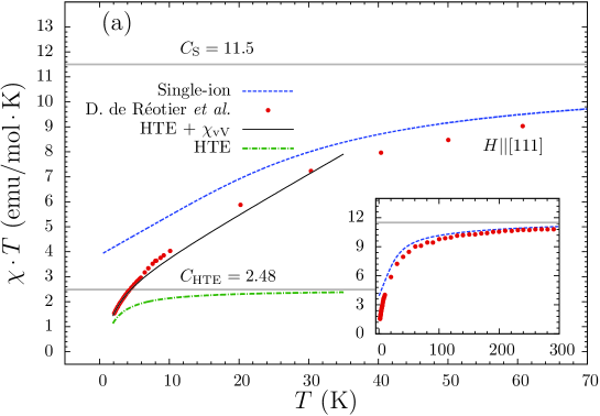
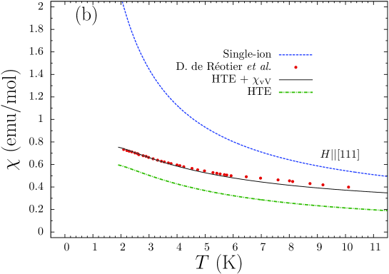
The inset of Fig. 3(a) shows a comparison of the measured susceptibility with . The agreement at high temperatures is apparent. The increasing disagreement between the experimental and the calculated as is reduced is caused by the progressive development of antiferromagnetic correlations which decrease the uniform susceptibility. The main plot shows that below about K, deviates significantly from the measured values. Also shown in Fig. 3(a) and Fig. 3(b) are comparisons with the susceptibility calculated by HTE for the projected spin- model (1) taken alone. The latter saturates to a Curie law form with at high temperatures. The HTE expansion considers AF correlations within the low-energy Hilbert space spanned by the single-ion crystal-field doublets of interacting Er3+ ions. These HTE calculations ignore the residual K temperature-independent contribution coming from the excited crystal-field states, which is the so-called van Vleck susceptibility, . White_book ; Jensen_book To compare experimental data with model calculations, we thus need to add to the HTE calculation results. As seen in Fig. 4(b), one obtains a very good agreement with the experimental data once is added.
Thermal ObD into Having demonstrated that the model in Eq. (1) describes the thermodynamic properties of the material above accurately, we now turn to the central question of thermal ObD at . We have already shown that the linear order-parameter susceptibility fails to distinguish between and order upon approaching from the paramagnetic phase. To further address this issue, we need to calculate non-linear order-parameter susceptibilities constructed from equal-time and power cumulants of the and order parameters in HTE. We find that the power cumulant is also identical for the two cases. However, the power of the order parameter does distinguish between and order (see Table VI in the supplementary materials supp_mater ). The necessity to compute a non-linear susceptibility that is order in the order-parameter to reveal the selection of vs can be understood on the basis that a order effective “potential”, , ( where and selects and , respectively) in the Ginzburg-Landau free-energy is dynamically generated by thermal and quantum fluctuations. Savary ; McClarty_ETO Starting at order , the non-linear order susceptibility for order (or ) gets larger than for for every () order considered. supp_mater This order susceptibility exposes a thermal order by disorder that coincides with the pattern of order selected at in the works of Savary et al.Savary and Zhitomirsky et al.Zhitomirsky (whose model is slightly different from the one we study).
Conclusion We have shown that the nearest-neighbor spin Hamiltonian (1), with exchange parameters determined from inelastic neutron scattering, Savary describes the thermodynamic properties of Er2Ti2O7 at , including the continuous phase transition at rather adequately. This was demonstrated through detailed comparison of calculated and experimental specific heat () and uniform susceptibility () data. While the nearest-neighbor part of the dipolar interactions is implicitly incorporated in the model, dipoles_in_nn it lacks such terms beyond nearest neighbors. In spite of that, the thermodynamic properties are described quite well. Similar conclusions were recently reached about a nearest-neighbor model determined by inelastic neutron scattering for the material Yb2Ti2O7. Ross ; Applegate ; Hayre
We have also shown that in the paramagnetic phase, the linear order-parameter susceptibility does not reveal the lifting of the manifold degeneracy. The selection of order is only evinced through a non-linear susceptibility that is order in the order-parameter. The thermal order-by-disorder identified in this paper was found to occur in the state, in agreement with experiments Champion_PRB ; Ruff_ETO_PRL ; Poole and with the quantum order-by-disorder calculations of Refs. [Savary, ; Zhitomirsky, ]. We thus conclude that the material Er2Ti2O7 presents a unique and convincing case of co-operating quantum and thermal order-by-disorder in a frustrated quantum antiferromagnet.
Acknowledgements.
We thank Behnam Javanparast, Anson Wong and Zhihao Hao for useful discussions. This work is supported in part by NSF grant number DMR-1004231 (RRPS), the NSERC of Canada, the Canada Research Chair program (M.G., Tier 1) and by the Perimeter Institute for Theoretical Physics.References
- (1) J. Villain, R. Bidaux, J.-P. Carton, and R. Conte, J. Phys. France 41, 1263 (1980).
- (2) E. F. Shender, Sov. Phys. JETP 56, 178 (1982).
- (3) R. Barnett, S. Powell, T. Grass, M. Lewenstein, and S. Das Sarma Phys. Rev. A 85, 023615 (2012), and references therein.
- (4) T. Yildirim, Turkish Journal of Physics 23, 47 (1999).
- (5) L. Savary, K. A. Ross, B. D. Gaulin, J. P. C. Ruff, and Leon Balents, Phys. Rev. Lett. 109, 167201 (2012).
- (6) J. D. M. Champion, M. J. Harris, P. C. W. Holdsworth, A. S. Wills, G. Balakrishnan, S. T. Bramwell, C. Čižmár, T. Fennell, J. S. Gardner, J. Lago, D. F. McMorrow, M. Orendáč, A. Orendáčová D. McK. Paul, R. I. Smith, M. T. F. Telling, and A. Wildes Phys. Rev. B 68, 020401 2004).
- (7) J. P. C. Ruff, J. P. Clancy, A. Bourque, M. A. White, M. Ramazanoglu, J. S. Gardner, Y. Qiu, J. R. D. Copley, M. B. Johnson, H. A. Dabkowska, and B. D. Gaulin Phys. Rev. Lett. 101, 147205 (2008).
- (8) A. Poole, A. S. Wills, and E. Lelièvre-Berna, Journal of Physics: Condensed Matter 19, 452201 (2007).
- (9) M. E. Zhitomirsky, M. V. Gvozdikova, P. C. W. Holdsworth, R. Moessner, Phys. Rev. Lett. 109, 077204 (2012).
- (10) S. E. Palmer and J. T. Chalker, Phys. Rev. B 62 488 (2000).
- (11) J. D. M. Champion and P. C. W. Holdsworth, Journal of Physics: Condensed Matter 16, S665 (2004).
- (12) P. Stasiak, P. A. McClarty, and M. J. P. Gingras, arXiv:1108.6053 (2011).
- (13) P. A. McClarty, S. H. Curnoe, and M. J. P. Gingras, Journal of Physics: Conference Series 145, 012032 (2009).
- (14) We omit here the tenuous energetic mechanism selection of discussed in Ref. [McClarty_ETO, ] and which involves a high-order van Vleck -like susceptibility.
- (15) The magnetostatic dipole-dipole interactions, written as , have their nearest-neighbor part implicitly incorporated in the parameters of in Eq. (1) and their contribution beyond nearest neighbors neglected.
- (16) It is possible in principle to have a different low-temperature state stabilized by q-ObD than the state found at that is selected by thermal ObD. For example, a double-transition sequence paramagnetic is observed in a classical Heisenberg pyrochlore antiferromagnet model with “indirect” Dzyaloshinskii-Moriya interactions. G.-W. Chern, arXiv:1008.3038 (2010).
- (17) See Supplementary Material.
- (18) K. A. Ross, Th. Proffen, H. A. Dabkowska, J. A. Quilliam, L. R. Yaraskavitch, J. B. Kycia, and B. D. Gaulin, Phys. Rev. B, 86, 174424 (2012).
- (19) J. S. Gardner, M. J. P. Gingras, and J. E. Greedan, Rev. Mod. Phys. 82, 53 (2010).
- (20) K. A. Ross, L. Savary, B. D. Gaulin and L. Balents, Phys. Rev. X 1, 021002 (2011).
- (21) The numerical values of those couplings are, (in Kelvin): , , and . The two largest couplings are of the type and the physics is thus very different from spin ice (see for example Ref.Ross ).
- (22) The components of entering in projected in the ground doublet are expressed as where are cartesian components and sum over repeated indices is implied. are the elements of the -tensor with principal axes along the local , and directions with eigenvalues and from Ref. [Savary, ].
- (23) J. Oitmaa, C. Hamer and W. Zheng, Series Expansion Methods for strongly interacting lattice models, Cambridge University Press (2006).
- (24) M. Rigol, T. Bryant and R. R. P. Singh, Phys. Rev. Lett. 97, 187202 (2006).
- (25) R. Applegate, N. R. Hayre, R. R. P. Singh, T. Lin, A. G. R. Day, and M. J. P. Gingras, Phys. Rev. Lett. 109, 097205 (2012).
- (26) N. R. Hayre, K. A. Ross, R. Applegate, T. Lin, R. R. P. Singh B. D. Gaulin, and M. J. P. Gingras, arXiv:1211.5934 (2012).
- (27) P. Dalmas de Réotier, A. Yaouanc, Y. Chapuis, S. H. Curnoe, B. Grenier, E. Ressouche, C. Marin, J. Lago, C. Baines, and S. R. Giblin, Phys. Rev. B 86, 104424 (2012).
- (28) S. S. Sosin, L. A. Prozorova, M. R. Lees, G. Balakrishnan, and O. A. Petrenko, Phys. Rev. B 82, 094428 (2010).
- (29) A. Bertin, Y. Chapuis, P. Dalmas de Réotier, and A Yaouanc. Journal of Physics: Condensed Matter 24, 256003 (2012).
- (30) R.M. White, Quantum Theory of Magnetism: Magnetic Properties of Materials, Springer Series in Solid-State Sciences. Springer (2010).
- (31) J. Jensen and A. R. Mackintosh, Rare Earth Magnetism, (Clarendon Press, Oxford, 1991).
- (32) The addition of pseudo-dipolar or indirect Dzyaloshinksii-Moriya interactions, such as those considered in Ref. [McClarty_ETO, ], renormalize the critical value of the magnetostatic dipolar interaction at which thermal ObD to occurs in Ref. [Stasiak, ] despite the ground state being Palmer-Chalker. Palmer_Chalker
- (33) A Monte Carlo study of a classical Heisenberg antiferromagnet model that interpolates between a face-centered cubic lattice and a pyrochlore found that the thermal order-by-disorder always overcomes the energetic selection down to the lowest temperature. [C. Pinettes, B. Canals, and C. Lacroix, Phys. Rev. B 66, 024422 (2002).]
- (34) We thank B. Gaulin, K. Ross and J. Ruff and K. Rule for correspondence on this matter.
I Supplemental Material
This section provides supplemental material to the main part of our paper. Firstly, we discuss the hypothetical situation when the thermal order-by-disorder can lead to a different long-range ordered state than the quantum order-by-disorder. Secondly, we provide some details regarding the high-temperature series expansion, in particular in regards to the order parameter linear and non-linear susceptibilities. Then we show the results for the temperature dependence of the magnetic entropy, , corresponding to the magnetic specific heat presented in the body of the paper. Finally, we provide tables for the high-temperature series expansion of various quantities of interest and referred to in the main text.
I.1 Metastability of States Selected by Thermal Order-by-Disorder
One may ask whether the long-range ordered state that is selected at the critical temperature differs from the zero-temperature ground state selected by quantum fluctuations. In case, thermal and quantum ObD are different, there is a possibility of metastability of the thermal ObD state at low temperatures. Thus, the concern here has to do with the kinetics in the real material rather than thermodynamics. Unlike natural proteins, extensively degenerate systems may lack funneled free-energy landscapes. As a result, configuration-space pathways and dynamical access to states may play a role in the specific long-range ordered phases experimentally realized. Ref. [Savary, ] finds a zero-point energy stabilization () of compared to of merely eV (a factor 1/30 of the reported smallest anisotropic exchange. Savary ) One may then ask whether the neglected interactions beyond nearest neighbors, in particular the dipolar interactions of magnitude 10 eV , dipoles_in_nn may have instead led to a ground state via quantum ObD. Meanwhile, thermal ObD, not considered in Ref. [Savary, ], may in fact be responsible for a transition into at , both in the material and in an amended version of the model of Ref. [Savary, ] that would incorporate interactions neglected therein. double_transition Following such a thermal ObD into in the material, a lower temperature ordering into , or even in the Palmer-Chalker state, may be dynamically inhibited, similar to what is found in Monte Carlo simulations of a pyrochlore antiferromagnet with weak dipolar interactions. Stasiak ; move_critical_dipole ; Pinettes In such a scenario, the model of Ref. Savary would seemingly predict the correct low-temperature state of Er2Ti2O7 but for the wrong reasons. To rule out the possibility of metastability of at low temperatures, one could cool down to a high-field phase and gradually lower the field at low temperatures to assess whether is still realized. To our knowledge, such an experiment has not been carried out. thx_field
I.2 Notes on High Temperature Series Expansion for Er2Ti2O7
We consider the Hamiltonian
| (3) |
Here is the exchange Hamiltonian defined in terms of local spin variables and exchange constants , , and . The next term is the Zeeman term arising from the applied external field which, for a field along , can be written in terms of local spin variables as
Here the subscripts , , and denote different sublattices and one needs to sum over all sites. The last two terms in the Hamiltonian are auxiliary field terms introduced for computational purposes.
| (5) |
and
| (6) |
All spins are defined in their local basis.
High temperature series expansions are calculated for the logarithm of the zero-field partition function , with given by
| (7) |
From the entropy and specific heat series follow by simple differentiation.
The zero field uniform susceptibility is calculated as the second derivative of the free energy with respect to the applied external magnetic field, , with .
| (8) |
In calculating from this equation, one obtains only the contribution from the interacting ions assumed to be in their single-ion crystal field ground states and neglecting any contribution from excited crystal field levels. To reach quantitative agreement with experiments, one needs to incorporate the residual low-temperature contribution to the susceptibility coming from the excited crystal field states. This is the so-called van Vleck susceptibility. White_book ; Jensen_book
To calculate the order-parameter susceptibility for , we set and calculate the second derivative of the free energy with respect to .
| (9) |
Similarly, for , order we set and take second derivative of free energy with respect to
| (10) |
Evidently the series for and are identical.
Non-linear susceptibilities do not appear to have linked-cluster property. Instead, higher order zero field cumulants were calculated by Linked cluster expansion. These are analogous to equal-time structure factors (rather than zero-frequency susceptibilities). Setting , we define for or the order-parameter operator
| (11) |
Then, the cumulants, , are:
| (12) |
| (13) |
and
| (14) |
Here, one should note that the bare moments and do not satisfy linked cluster property but the cumulants do. Since and are identical term by term, the difference is equal to the difference in the cumulants, .
II Temperature Dependence of the Magnetic Entropy,
The magnetic entropy function, , is shown in Fig. 4. We show the partial sums of the series from order 8 to order 12 as well as a few Padé approximants. At the critical temperature the entropy per mole in units of the perfect gas constant is around . In other words, it is reduced from the infinite temperature value, , by less than fifty percent. This is not unusual compared to typical three-dimensional phase transitions to long-range order. This indicates that the system is not highly frustrated with the development of a strongly correlated regime above . A similar conclusion was reached in Ref. [Savary, ] on the basis of a comparison between the mean-field critical temperature of the model, K, and the experimentally observed K
II.1 High-Temperature Series for Various Quantities
In this section, we provide the reader with tables of coefficients forthe high-temperature series of quantities of interest. Unless stated otherwise, the high-temperature series of a quantitity, , as a function of inverse temperature (with temperature in Kelvin), is expressed in the form
| (15) |
| Order | expansion coefficient |
|---|---|
| 0 | |
| 1 | |
| 2 | |
| 3 | |
| 4 | |
| 5 | |
| 6 | |
| 7 | |
| 8 | |
| 9 | |
| 10 | |
| 11 | |
| 12 | 3 |
| Order | expansion coefficient |
|---|---|
| 0 | |
| 1 | |
| 2 | |
| 3 | |
| 4 | |
| 5 | |
| 6 | |
| 7 | |
| 8 | |
| 9 | |
| 10 | |
| 11 | |
| 12 |
| Order | expansion coefficient |
|---|---|
| 0 | |
| 1 | |
| 2 | |
| 3 | |
| 4 | |
| 5 | |
| 6 | |
| 7 | |
| 8 |
| Order | expansion coefficient |
|---|---|
| 0 | |
| 1 | |
| 2 | |
| 3 | |
| 4 | |
| 5 | |
| 6 | |
| 7 | |
| 8 |
| Order | expansion coefficient |
|---|---|
| 0 | |
| 1 | |
| 2 | |
| 3 | |
| 4 | |
| 5 | |
| 6 | |
| 7 | |
| 8 |
| Order | expansion coefficient (-cumulant) | expansion coefficient (-cumulant) | difference |
|---|---|---|---|
| 0 | |||
| 1 | |||
| 2 | |||
| 3 | |||
| 4 | |||
| 5 | |||
| 6 | |||
| 7 | |||
| 8 |
| Order | expansion coefficient |
|---|---|
| 0 | |
| 1 | |
| 2 | |
| 3 | |
| 4 | |
| 5 | |
| 6 |