The Growth of Cool Cores and Evolution of Cooling Properties in a
Sample of 83 Galaxy Clusters at $0.3<z<1.2$ Selected from the SPT-SZ Survey

M. McDonald^$\dagger$^$\dagger$affiliation: Hubble Fellow ¹¹affiliation: Kavli Institute for Astrophysics and Space Research, Massachusetts Institute of Technology, 77 Massachusetts Avenue, Cambridge, MA 02139 , B. A. Benson²²affiliation: Kavli Institute for Cosmological Physics, University of Chicago, 5640 South Ellis Avenue, Chicago, IL 60637 ³³affiliation: Enrico Fermi Institute, University of Chicago, 5640 South Ellis Avenue, Chicago, IL 60637 , A. Vikhlinin⁴⁴affiliation: Harvard-Smithsonian Center for Astrophysics, 60 Garden Street, Cambridge, MA 02138 , B. Stalder⁴⁴affiliation: Harvard-Smithsonian Center for Astrophysics, 60 Garden Street, Cambridge, MA 02138 , L. E. Bleem²²affiliation: Kavli Institute for Cosmological Physics, University of Chicago, 5640 South Ellis Avenue, Chicago, IL 60637 ⁵⁵affiliation: Department of Physics, University of Chicago, 5640 South Ellis Avenue, Chicago, IL 60637 , T. de Haan⁶⁶affiliation: Department of Physics, McGill University, 3600 Rue University, Montreal, Quebec H3A 2T8, Canada , H. W. Lin⁷⁷affiliation: Caddo Parish Magnet High School, Shrevport, LA 71101 , K. A. Aird⁸⁸affiliation: University of Chicago, 5640 South Ellis Avenue, Chicago, IL 60637 , M. L. N. Ashby⁴⁴affiliation: Harvard-Smithsonian Center for Astrophysics, 60 Garden Street, Cambridge, MA 02138 , M. W. Bautz¹¹affiliation: Kavli Institute for Astrophysics and Space Research, Massachusetts Institute of Technology, 77 Massachusetts Avenue, Cambridge, MA 02139 , M. Bayliss⁴⁴affiliation: Harvard-Smithsonian Center for Astrophysics, 60 Garden Street, Cambridge, MA 02138 ⁹⁹affiliation: Department of Physics, Harvard University, 17 Oxford Street, Cambridge, MA 02138 , S. Bocquet¹⁰¹⁰affiliation: Department of Physics, Ludwig-Maximilians-Universität, Scheinerstr. 1, 81679 München, Germany ¹¹¹¹affiliation: Excellence Cluster Universe, Boltzmannstr. 2, 85748 Garching, Germany , M. Brodwin¹²¹²affiliation: Department of Physics and Astronomy, University of Missouri, 5110 Rockhill Road, Kansas City, MO 64110 , J. E. Carlstrom²²affiliation: Kavli Institute for Cosmological Physics, University of Chicago, 5640 South Ellis Avenue, Chicago, IL 60637 ⁵⁵affiliation: Department of Physics, University of Chicago, 5640 South Ellis Avenue, Chicago, IL 60637 ³³affiliation: Enrico Fermi Institute, University of Chicago, 5640 South Ellis Avenue, Chicago, IL 60637 ¹³¹³affiliation: Department of Astronomy and Astrophysics, University of Chicago, 5640 South Ellis Avenue, Chicago, IL 60637 ¹⁴¹⁴affiliation: Argonne National Laboratory, 9700 S. Cass Avenue, Argonne, IL, USA 60439 , C. L. Chang²²affiliation: Kavli Institute for Cosmological Physics, University of Chicago, 5640 South Ellis Avenue, Chicago, IL 60637 ³³affiliation: Enrico Fermi Institute, University of Chicago, 5640 South Ellis Avenue, Chicago, IL 60637 ¹⁴¹⁴affiliation: Argonne National Laboratory, 9700 S. Cass Avenue, Argonne, IL, USA 60439 , H. M. Cho¹⁵¹⁵affiliation: NIST Quantum Devices Group, 325 Broadway Mailcode 817.03, Boulder, CO, USA 80305 , A. Clocchiatti¹⁶¹⁶affiliation: Departamento de Astronomia y Astrosifica, Pontificia Universidad Catolica, Chile , T. M. Crawford²²affiliation: Kavli Institute for Cosmological Physics, University of Chicago, 5640 South Ellis Avenue, Chicago, IL 60637 ¹³¹³affiliation: Department of Astronomy and Astrophysics, University of Chicago, 5640 South Ellis Avenue, Chicago, IL 60637 , A. T. Crites²²affiliation: Kavli Institute for Cosmological Physics, University of Chicago, 5640 South Ellis Avenue, Chicago, IL 60637 ¹³¹³affiliation: Department of Astronomy and Astrophysics, University of Chicago, 5640 South Ellis Avenue, Chicago, IL 60637 , S. Desai¹⁰¹⁰affiliation: Department of Physics, Ludwig-Maximilians-Universität, Scheinerstr. 1, 81679 München, Germany ¹¹¹¹affiliation: Excellence Cluster Universe, Boltzmannstr. 2, 85748 Garching, Germany , M. A. Dobbs⁶⁶affiliation: Department of Physics, McGill University, 3600 Rue University, Montreal, Quebec H3A 2T8, Canada , J. P. Dudley⁶⁶affiliation: Department of Physics, McGill University, 3600 Rue University, Montreal, Quebec H3A 2T8, Canada , R. J. Foley⁴⁴affiliation: Harvard-Smithsonian Center for Astrophysics, 60 Garden Street, Cambridge, MA 02138 , W. R. Forman⁴⁴affiliation: Harvard-Smithsonian Center for Astrophysics, 60 Garden Street, Cambridge, MA 02138 , E. M. George¹⁷¹⁷affiliation: Department of Physics, University of California, Berkeley, CA 94720 , D. Gettings¹⁸¹⁸affiliation: Department of Astronomy, University of Florida, Gainesville, FL 32611 , M. D. Gladders²²affiliation: Kavli Institute for Cosmological Physics, University of Chicago, 5640 South Ellis Avenue, Chicago, IL 60637 ¹³¹³affiliation: Department of Astronomy and Astrophysics, University of Chicago, 5640 South Ellis Avenue, Chicago, IL 60637 , A. H. Gonzalez¹⁸¹⁸affiliation: Department of Astronomy, University of Florida, Gainesville, FL 32611 , N. W. Halverson¹⁹¹⁹affiliation: Department of Astrophysical and Planetary Sciences and Department of Physics, University of Colorado, Boulder, CO 80309 , F. W. High²²affiliation: Kavli Institute for Cosmological Physics, University of Chicago, 5640 South Ellis Avenue, Chicago, IL 60637 ¹³¹³affiliation: Department of Astronomy and Astrophysics, University of Chicago, 5640 South Ellis Avenue, Chicago, IL 60637 , G. P. Holder⁶⁶affiliation: Department of Physics, McGill University, 3600 Rue University, Montreal, Quebec H3A 2T8, Canada , W. L. Holzapfel¹⁷¹⁷affiliation: Department of Physics, University of California, Berkeley, CA 94720 , S. Hoover²²affiliation: Kavli Institute for Cosmological Physics, University of Chicago, 5640 South Ellis Avenue, Chicago, IL 60637 ³³affiliation: Enrico Fermi Institute, University of Chicago, 5640 South Ellis Avenue, Chicago, IL 60637 , J. D. Hrubes⁸⁸affiliation: University of Chicago, 5640 South Ellis Avenue, Chicago, IL 60637 , C. Jones⁴⁴affiliation: Harvard-Smithsonian Center for Astrophysics, 60 Garden Street, Cambridge, MA 02138 , M. Joy²⁰²⁰affiliation: Department of Space Science, VP62, NASA Marshall Space Flight Center, Huntsville, AL 35812 , R. Keisler²²affiliation: Kavli Institute for Cosmological Physics, University of Chicago, 5640 South Ellis Avenue, Chicago, IL 60637 ⁵⁵affiliation: Department of Physics, University of Chicago, 5640 South Ellis Avenue, Chicago, IL 60637 , L. Knox²¹²¹affiliation: Department of Physics, University of California, One Shields Avenue, Davis, CA 95616 , A. T. Lee¹⁷¹⁷affiliation: Department of Physics, University of California, Berkeley, CA 94720 ²²²²affiliation: Physics Division, Lawrence Berkeley National Laboratory, Berkeley, CA 94720 , E. M. Leitch²²affiliation: Kavli Institute for Cosmological Physics, University of Chicago, 5640 South Ellis Avenue, Chicago, IL 60637 ¹³¹³affiliation: Department of Astronomy and Astrophysics, University of Chicago, 5640 South Ellis Avenue, Chicago, IL 60637 , J. Liu¹⁰¹⁰affiliation: Department of Physics, Ludwig-Maximilians-Universität, Scheinerstr. 1, 81679 München, Germany ¹¹¹¹affiliation: Excellence Cluster Universe, Boltzmannstr. 2, 85748 Garching, Germany , M. Lueker¹⁷¹⁷affiliation: Department of Physics, University of California, Berkeley, CA 94720 ²³²³affiliation: California Institute of Technology, 1200 E. California Blvd., Pasadena, CA 91125 , D. Luong-Van⁸⁸affiliation: University of Chicago, 5640 South Ellis Avenue, Chicago, IL 60637 , A. Mantz²²affiliation: Kavli Institute for Cosmological Physics, University of Chicago, 5640 South Ellis Avenue, Chicago, IL 60637 , D. P. Marrone²⁴²⁴affiliation: Steward Observatory, University of Arizona, 933 North Cherry Avenue, Tucson, AZ 85721 , J. J. McMahon²⁵²⁵affiliation: Department of Physics, University of Michigan, 450 Church Street, Ann Arbor, MI, 48109 , J. Mehl²²affiliation: Kavli Institute for Cosmological Physics, University of Chicago, 5640 South Ellis Avenue, Chicago, IL 60637 ¹³¹³affiliation: Department of Astronomy and Astrophysics, University of Chicago, 5640 South Ellis Avenue, Chicago, IL 60637 ¹⁴¹⁴affiliation: Argonne National Laboratory, 9700 S. Cass Avenue, Argonne, IL, USA 60439 , S. S. Meyer²²affiliation: Kavli Institute for Cosmological Physics, University of Chicago, 5640 South Ellis Avenue, Chicago, IL 60637 ⁵⁵affiliation: Department of Physics, University of Chicago, 5640 South Ellis Avenue, Chicago, IL 60637 ³³affiliation: Enrico Fermi Institute, University of Chicago, 5640 South Ellis Avenue, Chicago, IL 60637 ¹³¹³affiliation: Department of Astronomy and Astrophysics, University of Chicago, 5640 South Ellis Avenue, Chicago, IL 60637 , E. D. Miller¹¹affiliation: Kavli Institute for Astrophysics and Space Research, Massachusetts Institute of Technology, 77 Massachusetts Avenue, Cambridge, MA 02139 , L. Mocanu²²affiliation: Kavli Institute for Cosmological Physics, University of Chicago, 5640 South Ellis Avenue, Chicago, IL 60637 ¹³¹³affiliation: Department of Astronomy and Astrophysics, University of Chicago, 5640 South Ellis Avenue, Chicago, IL 60637 , J. J. Mohr¹⁰¹⁰affiliation: Department of Physics, Ludwig-Maximilians-Universität, Scheinerstr. 1, 81679 München, Germany ¹¹¹¹affiliation: Excellence Cluster Universe, Boltzmannstr. 2, 85748 Garching, Germany ²⁶²⁶affiliation: Max-Planck-Institut für extraterrestrische Physik, Giessenbachstr. 85748 Garching, Germany , T. E. Montroy²⁷²⁷affiliation: Physics Department, Center for Education and Research in Cosmology and Astrophysics, Case Western Reserve University, Cleveland, OH 44106 , S. S. Murray⁴⁴affiliation: Harvard-Smithsonian Center for Astrophysics, 60 Garden Street, Cambridge, MA 02138 , D. Nurgaliev⁹⁹affiliation: Department of Physics, Harvard University, 17 Oxford Street, Cambridge, MA 02138 , S. Padin²²affiliation: Kavli Institute for Cosmological Physics, University of Chicago, 5640 South Ellis Avenue, Chicago, IL 60637 ¹³¹³affiliation: Department of Astronomy and Astrophysics, University of Chicago, 5640 South Ellis Avenue, Chicago, IL 60637 ²³²³affiliation: California Institute of Technology, 1200 E. California Blvd., Pasadena, CA 91125 , T. Plagge²²affiliation: Kavli Institute for Cosmological Physics, University of Chicago, 5640 South Ellis Avenue, Chicago, IL 60637 ¹³¹³affiliation: Department of Astronomy and Astrophysics, University of Chicago, 5640 South Ellis Avenue, Chicago, IL 60637 , C. Pryke²⁸²⁸affiliation: Physics Department, University of Minnesota, 116 Church Street S.E., Minneapolis, MN 55455 , C. L. Reichardt¹⁷¹⁷affiliation: Department of Physics, University of California, Berkeley, CA 94720 , A. Rest²⁹²⁹affiliation: Space Telescope Science Institute, 3700 San Martin Dr., Baltimore, MD 21218 , J. Ruel⁹⁹affiliation: Department of Physics, Harvard University, 17 Oxford Street, Cambridge, MA 02138 , J. E. Ruhl²⁷²⁷affiliation: Physics Department, Center for Education and Research in Cosmology and Astrophysics, Case Western Reserve University, Cleveland, OH 44106 , B. R. Saliwanchik²⁷²⁷affiliation: Physics Department, Center for Education and Research in Cosmology and Astrophysics, Case Western Reserve University, Cleveland, OH 44106 , A. Saro¹⁰¹⁰affiliation: Department of Physics, Ludwig-Maximilians-Universität, Scheinerstr. 1, 81679 München, Germany , J. T. Sayre²⁷²⁷affiliation: Physics Department, Center for Education and Research in Cosmology and Astrophysics, Case Western Reserve University, Cleveland, OH 44106 , K. K. Schaffer²²affiliation: Kavli Institute for Cosmological Physics, University of Chicago, 5640 South Ellis Avenue, Chicago, IL 60637 ³³affiliation: Enrico Fermi Institute, University of Chicago, 5640 South Ellis Avenue, Chicago, IL 60637 ³⁰³⁰affiliation: Liberal Arts Department, School of the Art Institute of Chicago, 112 S Michigan Ave, Chicago, IL 60603 , E. Shirokoff¹⁷¹⁷affiliation: Department of Physics, University of California, Berkeley, CA 94720 ²³²³affiliation: California Institute of Technology, 1200 E. California Blvd., Pasadena, CA 91125 , J. Song²⁵²⁵affiliation: Department of Physics, University of Michigan, 450 Church Street, Ann Arbor, MI, 48109 , R. Šuhada¹⁰¹⁰affiliation: Department of Physics, Ludwig-Maximilians-Universität, Scheinerstr. 1, 81679 München, Germany , H. G. Spieler²²²²affiliation: Physics Division, Lawrence Berkeley National Laboratory, Berkeley, CA 94720 , S. A. Stanford²¹²¹affiliation: Department of Physics, University of California, One Shields Avenue, Davis, CA 95616 ³¹³¹affiliation: Institute of Geophysics and Planetary Physics, Lawrence Livermore National Laboratory, Livermore, CA 94551 , Z. Staniszewski²⁷²⁷affiliation: Physics Department, Center for Education and Research in Cosmology and Astrophysics, Case Western Reserve University, Cleveland, OH 44106 , A. A. Stark⁴⁴affiliation: Harvard-Smithsonian Center for Astrophysics, 60 Garden Street, Cambridge, MA 02138 , K. Story²²affiliation: Kavli Institute for Cosmological Physics, University of Chicago, 5640 South Ellis Avenue, Chicago, IL 60637 ⁵⁵affiliation: Department of Physics, University of Chicago, 5640 South Ellis Avenue, Chicago, IL 60637 , A. van Engelen⁶⁶affiliation: Department of Physics, McGill University, 3600 Rue University, Montreal, Quebec H3A 2T8, Canada , K. Vanderlinde³²³²affiliation: Dunlap Institute for Astronomy & Astrophysics, University of Toronto, 50 St George St, Toronto, ON, M5S 3H4, Canada ³³³³affiliation: Department of Astronomy & Astrophysics, University of Toronto, 50 St George St, Toronto, ON, M5S 3H4, Canada , J. D. Vieira²²affiliation: Kavli Institute for Cosmological Physics, University of Chicago, 5640 South Ellis Avenue, Chicago, IL 60637 ⁵⁵affiliation: Department of Physics, University of Chicago, 5640 South Ellis Avenue, Chicago, IL 60637 ²³²³affiliation: California Institute of Technology, 1200 E. California Blvd., Pasadena, CA 91125 , R. Williamson²²affiliation: Kavli Institute for Cosmological Physics, University of Chicago, 5640 South Ellis Avenue, Chicago, IL 60637 ¹³¹³affiliation: Department of Astronomy and Astrophysics, University of Chicago, 5640 South Ellis Avenue, Chicago, IL 60637 , O. Zahn¹⁷¹⁷affiliation: Department of Physics, University of California, Berkeley, CA 94720 ³⁴³⁴affiliation: Berkeley Center for Cosmological Physics, Department of Physics, University of California, and Lawrence Berkeley National Labs, Berkeley, CA 94720 , and A. Zenteno¹⁰¹⁰affiliation: Department of Physics, Ludwig-Maximilians-Universität, Scheinerstr. 1, 81679 München, Germany ¹¹¹¹affiliation: Excellence Cluster Universe, Boltzmannstr. 2, 85748 Garching, Germany Email: mcdonald@space.mit.edu

Abstract

We present first results on the cooling properties derived from Chandra X-ray observations of 83 high-redshift ( $0.3<z<1.2$ ) massive galaxy clusters selected by their Sunyaev-Zel’dovich signature in the South Pole Telescope data. We measure each cluster’s central cooling time, central entropy, and mass deposition rate, and compare these properties to those for local cluster samples. We find no significant evolution from $z\sim 0$ to $z\sim 1$ in the distribution of these properties, suggesting that cooling in cluster cores is stable over long periods of time. We also find that the average cool core entropy profile in the inner $\sim$ 100 kpc has not changed dramatically since z $\sim$ 1, implying that feedback must be providing nearly constant energy injection to maintain the observed “entropy floor” at $\sim$ 10 keV cm². While the cooling properties appear roughly constant over long periods of time, we observe strong evolution in the gas density profile, with the normalized central density ( $\rho_{g,0}/\rho_{\textrm{crit}}$ ) increasing by an order of magnitude from $z\sim 1$ to $z\sim 0$ . When using metrics defined by the inner surface brightness profile of clusters, we find an apparent lack of classical, cuspy, cool-core clusters at $z>0.75$ , consistent with earlier reports for clusters at $z>0.5$ using similar definitions. Our measurements indicate that cool cores have been steadily growing over the 8 Gyr spanned by our sample, consistent with a constant, $\sim$ 150 M_⊙ yr^-1 cooling flow that is unable to cool below entropies of 10 keV cm² and, instead, accumulates in the cluster center. We estimate that cool cores began to assemble in these massive systems at $z_{\textrm{cool}}=1.0^{+1.0}_{-0.2}$ , which represents the first constraints on the onset of cooling in galaxy cluster cores. At high redshift ( $z\gtrsim 0.75$ ), galaxy clusters may be classified as “cooling flows” (low central entropy, cooling time) but not “cool cores” (cuspy surface brightness profile), meaning that care must be taken when classifying these high- $z$ systems. We investigate several potential biases that could conspire to mimic this cool core evolution and are unable to find a bias that has a similar redshift dependence and a substantial amplitude.

Subject headings:

galaxies: clusters: general – galaxies: clusters: intracluster medium – cosmology: early universe – X-rays: galaxies: clusters

1. Introduction

In the inner $\sim$ 100 kpc of a galaxy cluster, the hot (10 ${}^{7}-10^{8}$ K) intracluster medium is often sufficiently dense that the cooling time, which is roughly $t_{cool}\propto T_{\rm{x}}^{1/2}n_{e}^{-1}$ , is shorter than a Hubble time. In these so-called “cool core” clusters, cooling gas should sink toward the center of the cluster, establishing a cooling flow which could deposit as much as $\sim$ 1000 M_⊙ yr^-1 of cold gas onto the central brightest cluster galaxy (for a review, see Fabian, 1994). The fact that brightest cluster galaxies (hereafter BCGs) are rarely forming stars at such prodigious rates (with the exception of the newly-discovered Phoenix cluster; McDonald et al. 2012, 2013) is prime evidence that some form of feedback offsets this cooling. The most likely culprit is mechanical feedback from the central active galactic nucleus (AGN; see Churazov et al., 2001; McNamara & Nulsen, 2007, 2012; Fabian, 2012), although other heat sources such as particle heating (Mathews, 2009), blazars (Pfrommer et al., 2012), and mergers (Gómez et al., 2002) are also viable.

If the balance between energy input from feedback and energy loss due to cooling is not exact, one would expect a residual cooling flow to develop. There is substantial evidence for such “reduced cooling flows”. Clumps and filaments of cooling intracluster gas have been detected at 10⁶–10⁷ K in the cores of clusters via high resolution X-ray spectroscopy (e.g., Peterson & Fabian, 2006; Sanders et al., 2010) and OVI emission in the far ultraviolet (e.g., Bregman et al., 2001; Oegerle et al., 2001; Bregman et al., 2006). Sparks et al. (2012) recently reported evidence for 10⁵ K gas (as traced by the C IV $\lambda$ 1549Å emission line) in the core of the Virgo cluster. Warm (10⁴ K) gas is nearly ubiquitous in cool core clusters (e.g., Hu et al., 1985; Johnstone et al., 1987; Heckman et al., 1989; Crawford et al., 1999; Edwards et al., 2007; Hatch et al., 2007; McDonald et al., 2010, 2011a), as are both warm (e.g., Jaffe et al., 2005; Edge et al., 2010; Donahue et al., 2011; Lim et al., 2012) and cold (e.g., Edge, 2001; Edge & Frayer, 2003; Salomé & Combes, 2003; Salomé et al., 2008; Lim et al., 2008; McDonald et al., 2012a) molecular gas components. Finally, perhaps the most convincing evidence that a fraction of the cooling intracluster medium (ICM) is reaching low temperatures is the fact that nearly all cool core clusters have star-forming BCGs, with star formation rates that correlate with the ICM cooling rate (e.g., McNamara & O’Connell, 1989; O’Dea et al., 2008; Rafferty et al., 2008; Donahue et al., 2010; Hicks et al., 2010; McDonald et al., 2011b). Thus, while there is significant evidence that some form of feedback is offsetting a large fraction of energy loss due to cooling in the ICM, it is also clear that this balance is imperfect and likely to vary on both short (periodic outbursts) and long (evolution) timescales.

While the physical processes that conspire to prevent or allow the formation of a dense, cool core in the ICM are not fully understood, there has been significant effort towards understanding the overall properties of these systems. Early, large surveys, including those by White et al. (1997), Peres et al. (1998), and Allen (2000), have formed the basis of our understanding of cooling flows (or lack thereof). These studies established the distribution of cooling properties, including the mass deposition rate, the cooling radius, and the central cooling time, for large X-ray flux-limited samples of nearby galaxy clusters. These studies showed that, among other things, clusters with strong cooling signatures tend to have multi-phase (i.e., H $\alpha$ -emitting) gas, radio-loud BCGs, and cooling rates that correlate with the total X-ray luminosity. Studies mentioned in the previous paragraph have largely built upon these early, pioneering works to classify the cooling properties of the intracluster medium.

While the properties of nearby ( $z\lesssim 0.3$ ) cool core clusters are well documented, very little is presently known about how cooling flows have evolved. Early work by Donahue et al. (1992) reported that, while the general properties of cooling flows appear to be unchanged since $z\sim 0.3$ , cool cores were more common by roughly a factor of two at this epoch. More recently, utilizing higher quality data from the Chandra X-ray Observatory, as well as ground-based optical data, on much larger, more complete samples, various studies have found evidence that there may be a decline in the fraction of clusters harboring strong (cuspy) cool cores with increasing redshift (Vikhlinin et al., 2007; Santos et al., 2010; Samuele et al., 2011; McDonald, 2011). These studies all report cool core fractions $\lesssim$ 10% at $z\gtrsim 0.5$ , indicating that cool core clusters are a recent phenomenon. Indeed, only a small number of clusters with strong cool cores are known at $z>0.5$ (e.g., Siemiginowska et al., 2010; Russell et al., 2012; Santos et al., 2012; McDonald et al., 2012b). It has been suggested that, since most of these samples were drawn from early surveys with the ROSAT X-ray telescope, they may be biased against cool cores at high redshifts due to their point-like appearance compared to the ROSAT resolution. The fact that optically-selected samples (McDonald, 2011) show the same evolution suggests that such a bias may not be a serious issue.

One significant issue affecting our understanding of the evolution of ICM cooling is the lack of large samples of high-redshift clusters with a well understood selection. The South Pole Telescope (SPT; Carlstrom et al., 2011) recently completed a 2500 square degree survey that has discovered hundreds of massive, high-redshift clusters using the Sunyaev-Zel’dovich (SZ; Sunyaev & Zeldovich, 1972) effect. Unlike X-ray and optical surveys, which have strong surface brightness biases, the SPT selection is nearly redshift-independent (at $z>0.3$ , see Song et al., 2012; Reichardt et al., 2013) and, based on simulations, is not expected to be significantly biased by the presence of cool cores (Motl et al., 2005; Pipino & Pierpaoli, 2010, Lin et al. in prep). In principle, such a survey should be able to trace the evolution of cool cores in the most massive clusters out to $z>1$ . Indeed, Semler et al. (2012) showed, in a pilot study of 13 SPT-selected clusters, that there is a significant population of cool core clusters at $z>0.5$ , contrary to the majority of the results reported in the literature at the time. Furthermore, the most extreme cool core cluster known is at $z=0.597$ , the Phoenix cluster (SPT-CLJ2344-4243; McDonald et al., 2012b), and was discovered by the SPT. Taken together, these results suggest that ICM cooling has not changed drastically in the past $\sim$ 8 Gyr.

In this work, we expand significantly on Semler et al. (2012), presenting Chandra X-ray observations of 83 massive, SPT-selected clusters. The majority of these observations were completed as part of a recent Chandra X-ray Visionary Project (PI B. Benson). With these data we are able to address two outstanding questions about the evolution of the cooling intracluster medium: i) Were cool cores less common at $z>0.5$ ? and ii) How have the properties of cooling flows evolved in the most massive galaxy clusters over the past $\sim$ 8 Gyr? In §2 we present the sample, describing first the selection and observations, followed by the analysis. In §3 we present the major results of this work, following in spirit the early works of White et al. (1997) and Peres et al. (1998) which identified the cooling flow properties of low-redshift, X-ray selected clusters. The implications of these results are discussed in §4. Throughout this work, we assume H₀=70 km s^-1 Mpc^-1, $\Omega_{M}$ = 0.27, and $\Omega_{\Lambda}$ = 0.73.

2. Data and Analysis

2.1. Sample Definition

The clusters used in this work were selected based on their Sunyaev-Zel’dovich (SZ) signature in the 2500 deg² SPT-SZ survey. The SPT-SZ survey was completed in November 2011, producing maps in three frequency bands (95, 150, and 220 GHz), with a key science goal of discovering clusters via the SZ effect (Staniszewski et al., 2009; Vanderlinde et al., 2010; Williamson et al., 2011; Benson et al., 2013; Reichardt et al., 2013).

The clusters considered in this work have additionally been observed with the Chandra X-ray Observatory, with exposures typically sufficient to obtain $\sim$ 2000 X-ray source counts. The majority of the clusters have been observed through a Chandra X-ray Visionary Project to obtain X-ray imaging of the 80 clusters detected with the highest SZ significance ( $\xi$ ) in the first 2000 deg² of the 2500 deg² SPT-SZ survey at $z>0.4$ (hereafter B13; Benson et al. in prep.) While B13 analyze the full XVP sample, we exclude six of the 80 clusters only observed with XMM-Newton, which does not have sufficient angular resolution to resolve the cool cores in typical high-redshift clusters. In addition, we include nine clusters at $z>0.3$ also detected in the SPT-SZ survey that were observed by Chandra, a sub-sample that primarily consists of clusters observed either in previous Chandra GO and GTO proposals from the SPT-SZ collaboration, or in other proposals to observe SZ-selected clusters from the Atacama Cosmology Telescope (ACT; Marriage et al., 2011) and Planck (Planck Collaboration et al., 2011) collaborations. We note that every SPT-selected cluster that was targeted with Chandra yielded an X-ray detection – perhaps unsurprising due to the dependence of both techniques on a rich ICM.

The final sample used in this work, referred to hereafter as SPT-XVP, is summarized in Table 1. The sample consists of 83 clusters, spanning a redshift range of $0.3<z<1.2$ and a mass range of $\sim 2\times 10^{14}<$ M ${}_{500}<20\times 10^{14}$ M ${}_{\odot}/h_{70}$ . The clusters were all identified in the SPT-SZ survey maps with a SPT detection significance, $\xi$ , spanning a range from $5.7<\xi<43$ . As was done in Vanderlinde et al. (2010), we predict the SPT survey completeness using cosmological and scaling relation constraints of the $\xi$ -mass relation. We assume the $\Lambda$ CDM cosmological constraints from Reichardt et al. (2013) when using a CMB data set and the SPT cluster catalog. At our median redshift of $z\sim 0.7$ , the SPT-XVP sample is expected to be $\sim$ 50% complete at $M_{500}=4\times 10^{14}M_{\odot}/h_{70}$ and nearly 100% complete at $6\times 10^{14}M_{\odot}/h_{70}$ . These completeness thresholds are nearly redshift independent, varying by $\lesssim$ 15% over the redshift range of the sample.

Name	$\alpha$ [^∘]	$\delta$ [^∘]	OBSIDs
SPT-CLJ0000-5748	0.250	-57.809	9335
SPT-CLJ0013-4906	3.331	-49.116	13462
SPT-CLJ0014-4952	3.690	-49.881	13471
SPT-CLJ0033-6326	8.469	-63.444	13483
SPT-CLJ0037-5047	9.447	-50.788	13493
SPT-CLJ0040-4407	10.208	-44.132	13395
SPT-CLJ0058-6145	14.586	-61.768	13479
SPT-CLJ0102-4603	15.677	-46.072	13485
SPT-CLJ0102-4915	15.734	-49.266	12258
SPT-CLJ0123-4821	20.796	-48.358	13491
SPT-CLJ0142-5032	25.546	-50.540	13467
SPT-CLJ0151-5954	27.857	-59.908	13480
SPT-CLJ0156-5541	29.042	-55.698	13489
SPT-CLJ0200-4852	30.141	-48.872	13487
SPT-CLJ0212-4657	33.108	-46.950	13464
SPT-CLJ0217-5245	34.304	-52.763	12269
SPT-CLJ0232-5257	38.202	-52.953	12263
SPT-CLJ0234-5831	38.677	-58.523	13403
SPT-CLJ0236-4938	39.258	-49.637	12266
SPT-CLJ0243-5930	40.865	-59.515	13484,15573
SPT-CLJ0252-4824	43.212	-48.415	13494
SPT-CLJ0256-5617	44.106	-56.298	13481,14448
SPT-CLJ0304-4401	46.067	-44.033	13402
SPT-CLJ0304-4921	46.067	-49.357	12265
SPT-CLJ0307-5042	46.961	-50.705	13476
SPT-CLJ0307-6225	46.830	-62.436	12191
SPT-CLJ0310-4647	47.634	-46.785	13492
SPT-CLJ0324-6236	51.053	-62.598	12181,13137,13213
SPT-CLJ0330-5228	52.728	-52.473	0893
SPT-CLJ0334-4659	53.547	-46.996	13470
SPT-CLJ0346-5439	56.733	-54.649	12270
SPT-CLJ0348-4515	57.075	-45.247	13465
SPT-CLJ0352-5647	58.241	-56.798	13490,15571
SPT-CLJ0406-4805	61.731	-48.082	13477
SPT-CLJ0411-4819	62.814	-48.320	13396
SPT-CLJ0417-4748	64.347	-47.813	13397
SPT-CLJ0426-5455	66.520	-54.918	13472
SPT-CLJ0438-5419	69.575	-54.322	12259
SPT-CLJ0441-4855	70.451	-48.924	13475,14371,14372
SPT-CLJ0446-5849	71.514	-58.830	13482,15560
SPT-CLJ0449-4901	72.275	-49.025	13473
SPT-CLJ0456-5116	74.118	-51.278	13474
SPT-CLJ0509-5342	77.339	-53.704	9432
SPT-CLJ0528-5300	82.023	-52.998	11747,11874,12092,13126
SPT-CLJ0533-5005	83.406	-50.096	11748,12001,12002
SPT-CLJ0542-4100	85.709	-41.000	0914
SPT-CLJ0546-5345^a	86.655	-53.759	9332,9336
SPT-CLJ0551-5709	87.896	-57.147	11743,11871
SPT-CLJ0555-6406	88.864	-64.105	13404
SPT-CLJ0559-5249	89.933	-52.827	12264,13116,13117
SPT-CLJ0616-5227	94.144	-52.453	12261,13127
SPT-CLJ0655-5234	103.974	-52.568	13486
SPT-CLJ2031-4037	307.966	-40.623	13517
SPT-CLJ2034-5936	308.537	-59.605	12182
SPT-CLJ2035-5251	308.793	-52.855	13466
SPT-CLJ2043-5035	310.823	-50.592	13478
SPT-CLJ2106-5844^b	316.518	-58.743	12180
SPT-CLJ2135-5726	323.912	-57.439	13463
SPT-CLJ2145-5644	326.468	-56.749	13398
SPT-CLJ2146-4632	326.645	-46.549	13469
SPT-CLJ2148-6116	327.181	-61.279	13488
SPT-CLJ2218-4519	334.746	-45.316	13501
SPT-CLJ2222-4834	335.712	-48.577	13497
SPT-CLJ2232-5959	338.141	-59.998	13502
SPT-CLJ2233-5339	338.319	-53.654	13504
SPT-CLJ2236-4555	339.219	-45.930	13507,15266
SPT-CLJ2245-6206	341.260	-62.116	13499
SPT-CLJ2248-4431	342.183	-44.530	4966
SPT-CLJ2258-4044	344.706	-40.740	13495
SPT-CLJ2259-6057	344.752	-60.960	13498
SPT-CLJ2301-4023	345.471	-40.389	13505
SPT-CLJ2306-6505	346.734	-65.090	13503
SPT-CLJ2325-4111	351.302	-41.196	13405
SPT-CLJ2331-5051	352.963	-50.865	9333
SPT-CLJ2335-4544	353.785	-45.739	13496
SPT-CLJ2337-5942	354.352	-59.706	11859
SPT-CLJ2341-5119	355.300	-51.329	11799
SPT-CLJ2342-5411	355.692	-54.185	11741,11870,12014,12091
SPT-CLJ2344-4243^c	356.183	-42.720	13401
SPT-CLJ2345-6405	356.250	-64.099	13500
SPT-CLJ2352-4657	358.068	-46.960	13506
SPT-CLJ2355-5055	358.948	-50.928	11746
SPT-CLJ2359-5009	359.933	-50.170	9334,11742,11864,11997
Table 1. Summary of Chandra X-ray observations. Positions listed
here are of the X-ray centroid (§2.2). The fourth column provides
the observational IDs from the Chandra X-ray Observatory.
^a: Brodwin et al. (2010)
^b: Foley et al. (2011)
^c: McDonald et al. (2012b)

2.2. Data Reduction and Analysis

Our basic data reduction and analysis follows closely that outlined in Vikhlinin et al. (2005) and Andersson et al. (2011). Briefly, this procedure includes filtering for background flares, applying the latest calibration corrections, and determining the appropriate blank sky background. In addition to using blank-sky backgrounds, we simultaneously model additional background components from Galactic sources as well as unresolved cosmic X-ray background (CXB) sources in off-source regions. Point sources were identified using an automated routine following a wavelet decomposition technique (Vikhlinin et al., 1998), and then visually inspected. Clumpy, asymmetric substructure was masked by hand, and excluded in calculations of the global temperature. The center of the cluster was chosen by iteratively measuring the centroid in a 250–500 kpc annulus. This choice, rather than the peak of emission, can play a significant role in whether or not the cluster is ultimately classified as a cool core or not – a subject we will return to in §4.

Global cluster properties (L_X,500, M₅₀₀, T_X,500, M_g,500) used in this work are derived in B13, following closely the procedures described in Andersson et al. (2011). For each of these quantities, the subscript refers to the quantity measured within R₅₀₀ – the radius within which the average enclosed density is 500 times the critical density. We estimate R₅₀₀ by requiring the measured quantities (T_X, M_g, Y_X) to satisfy a set of scaling relations between T_X,500, M_g,500, and Y_X,500 and M₅₀₀ (Vikhlinin et al., 2009). Each of these three scaling relations are individually satisfied by iteratively adjusting R₅₀₀. In this paper, we use R₅₀₀ from the Y_X–M relation only. Further details on both the data reduction and the derivation of global X-ray properties can be found in Vikhlinin et al. (2005) and Andersson et al. (2011), respectively.

2.3. Surface Brightness Profiles and Concentration Measurements

The surface brightness profile for each cluster, extracted in the energy range 0.7–2.0 keV, is measured in a series of 20 annuli, with the outer radii for each annulus defined as:

r_{i}=1.5\textrm{R}_{500}\left(\frac{i}{20}\right)^{1.5}~{}~{}~{}i=1...n~{}.

(1)

Following the techniques described in Vikhlinin et al. (2006), we correct these surface brightness profiles for spatial variations in temperature, metallicity, and the telescope effective area. Calibrated surface brightness profiles (see Appendix A) are expressed as a projected emission measure integral, $\int n_{e}n_{p}dl$ , where $n_{e}$ and $n_{p}$ are the electron and proton densities, respectively. We model the calibrated surface brightness profile with a modified beta model:

n_{e}n_{p}=n_{0}^{2}\frac{(r/r_{c})^{-\alpha}}{(1+r^{2}/r_{c}^{2})^{3\beta-\alpha/2}}\frac{1}{(1+r^{3}/r_{s}^{3})^{\epsilon/3}},

(2)

where $n_{0}$ is the core density, and $r_{c}$ and $r_{s}$ are scaling radii of the core and extended components, following Vikhlinin et al. (2006). This 3-dimensional model is numerically projected along the line of sight, yielding a model emission measure profile that is fit to the data. We estimate the 3-dimensional gas density assuming $n_{e}=Zn_{p}$ and $\rho_{g}=m_{p}n_{e}A/Z$ , where $A=1.397$ and $Z=1.199$ are the average nuclear charge and mass, respectively, for a plasma with metal abundance 30% of solar (0.3 $Z_{\odot}$ ). The calibrated surface brightness profiles and best-fit projected gas density models for the full sample are shown in Appendix A.

In recent studies of high-redshift cool core clusters (e.g., Vikhlinin et al., 2007; Santos et al., 2008, 2010; Semler et al., 2012), the presence of a cool core has been quantified solely by the central cuspiness of the surface brightness profile. While measuring the central deprojected temperature and cooling time typically requires $>$ 10,000 X-ray counts, the surface brightness profile can often be constrained in the central region with as few as $\sim$ 500 counts, making this an inexpensive method of classifying cool cores. To classify a sample of high-redshift clusters as cool core or non-cool core, Vikhlinin et al. (2007) defined a “cuspiness” parameter,

\alpha\equiv\left.\frac{d\log\rho_{g}}{d\log r}\right|_{r=0.04\textrm{R}_{500}}

(3)

This parameter has been shown to correlate well with the central cooling time for galaxy clusters at $z\sim 0$ (Vikhlinin et al., 2007; Hudson et al., 2010). Vikhlinin et al. (2007) showed that $\alpha$ was typically higher for a low-redshift sample of clusters ( $z<0.5$ ), suggesting a rapid evolution in cool core strength (Vikhlinin et al., 2007). While easily measurable, this parameter has the drawback that it assumes that the cool core radius evolves at the same rate as the cluster radius (R₅₀₀).

An alternative measure of the surface brightness cuspiness is the “concentration” parameter, as defined by Santos et al. (2008):

c_{SB}\equiv\frac{F_{0.5-5.0\rm{keV}}(r<40~{}\rm{kpc})}{F_{0.5-5.0\rm{keV}}(r<400~{}\rm{kpc})},

(4)

where $F_{0.5-5.0\rm{keV}}$ is the X-ray flux in the energy bandpass 0.5–5.0 keV. This value can range from $\sim$ 0 (no flux peak), to 1 (all flux in central 40 kpc). This choice of parameter is relatively insensitive to redshift effects, such as worsening spatial resolution, reduced counts, and $k$ -corrections (Santos et al., 2008), but has the potential drawback that it assumes no evolution in the cooling radius.

We will use both the full 3-dimensional density profile ( $n_{e}(r)$ ), as well as the commonly-used single-parameter estimates of profile peakedness ( $\alpha$ , $c_{SB}$ ) to trace the evolution of cool cores in this unique sample.

2.4. Deprojecting Radial X-ray Profiles

2.4.1 $\rho_{g}(r)$ , $\Phi(r)$ , T ${}_{X}(r)$

Many recent works have verified the presence, or lack, of high-redshift cool cores via surface brightness quantities, as discussed in the previous section. We wish to extend this analysis further and quantify the cooling properties of the ICM. With only $\sim$ 2000 X-ray counts per cluster, we cannot perform a full temperature and density deprojection analysis, as is typically done at low redshift (e.g., Vikhlinin et al., 2006; Sun et al., 2009). Instead, motivated by earlier studies with the Einstein X-ray observatory (White et al., 1997; Peres et al., 1998), we combine our knowledge of the X-ray surface brightness and a coarse temperature profile with assumptions about the underlying dark matter distribution to produce best-guess 3-dimensional temperature profiles. This procedure, which will be described in complete detail in an upcoming paper (McDonald et al. in prep), is summarized below.

First, a 3-bin temperature profile is derived by extracting X-ray spectra in logarithmically-spaced annuli over the range $0<r<\rm{R}_{500}$ . These spectra were fit in xspec (Arnaud, 1996) with a combined phabs(mekal) model²²2http://heasarc.gsfc.nasa.gov/docs/xanadu/xspec/manual/
XspecModels.html. In cases requiring additional background components, as determined from off-source regions of the field (see B13 for more details), an additional mekal (Galactic) or bremss (CXB) component was used, with temperatures fixed to 0.18 keV and 40 keV, respectively. For the source model, we fix the abundance to $0.3Z_{\odot}$ and the hydrogen absorbing column, n_H, to the average from the Leiden-Argentine-Bonn survey (Kalberla et al., 2005). The resulting temperature profiles for the full sample are shown in Appendix A.

In order to model the underlying dark matter potential, we use a generalized Navarro-Frenk-White (GNFW; Zhao, 1996; Wyithe et al., 2001) profile:

\rho_{D}=\frac{\rho_{D,0}}{(r/r_{s})^{\beta_{D}}(1+r/r_{s})^{3-\beta_{D}}},

(5)

where $\rho_{D,0}$ is the central dark matter density, $r_{s}$ is a scale radius related to the halo concentration by $C=\rm{R}_{200}/r_{s}$ , and $\beta_{D}$ is the inner slope of the dark matter profile. This model is similar to the NFW (Navarro et al., 1997) profile at large radii, but has a free “cuspiness” parameter at small radii. We estimate the initial values of $\rho_{D,0}$ and $r_{s}$ using the measured M₅₀₀ and the mass-concentration relation (Duffy et al., 2008).

Given an assumed 3-dimensional functional form of both the dark matter (Eq. 5) and gas density profiles (§2.3, Eq. 2), and further assuming a negligible contribution from stars to the total mass, we can derive the 3-dimensional temperature profile by combining hydrostatic equilibrium,

\frac{d\textrm{P}}{dr}=-\frac{\textrm{GM}(r)\rho(r)}{r^{2}},

(6)

with the ideal gas law (P $=n_{T}k$ T, where $n_{T}=n_{e}+n_{p}$ ). This temperature profile is projected along the line of sight (weighted by $n_{e}^{2}$ T^1/2), producing a 2-dimensional temperature profile which is compared to the data, allowing a calculation of $\chi^{2}$ . We repeat this process, varying both the normalization of the GNFW halo ( $\rho_{D,0}$ ), and thus the total dark matter mass, as well as the inner slope ( $\beta_{D}$ ), while requiring that the mass–concentration (Duffy et al., 2008) and M₅₀₀–P₅₀₀ (Nagai et al., 2007) relations are always satisfied (removing $r_{s}$ and P₅₀₀ as free parameters), until a stable minimum in the $\chi^{2}$ ( $\rho_{D,0}$ , $\beta_{D}$ ) plane is found. The net result of this process is a 3-dimensional model of the gas density, gas temperature, and gravitational potential for each cluster (see Appendix A).

2.4.2 $t_{\textrm{cool}}(r)$ , K $(r)$ , Ṁ $(r)$

While a centrally-concentrated surface brightness profile is an excellent indicator that the ICM is cooling rapidly (e.g., Hudson et al., 2010), we ultimately would like to quantify, in an absolute sense, the strength of this cooling. Classically, clusters have been identified as “cooling flows” if the cooling time in the central region is less than the age of the Universe, with the cooling time defined as:

t_{\textrm{cool}}=\frac{3}{2}\frac{n_{T}k\rm{T}}{n_{e}n_{H}\Lambda(\rm{T,Z})},

(7)

where $\Lambda(\rm{T,Z})$ is the cooling function for an optically-thin plasma (Sutherland & Dopita, 1993). Similarly, the specific entropy of the gas is defined as:

\textrm{K}=\frac{k\textrm{T}}{n_{e}^{2/3}}.

(8)

Both the central cooling time and central entropy are smallest in the centers of cool core clusters, and are distributed bimodally over the full cluster population (e.g., Cavagnolo et al., 2009; Hudson et al., 2010). In nearby, well-studied clusters, the central cooling time and entropy are well-defined, as both of these functions tend to flatten at radii less than $\sim$ 10 kpc. However, for lower signal-to-noise data, the measurement of central cooling time is strongly dependent on the choice of bin size (see e.g., White et al., 1997; Peres et al., 1998), and inwards extrapolation can be risky if a flattening of the surface brightness profile is not observed due to poor spatial sampling. For this work, we choose as our central bin $r<0.012\textrm{R}_{500}$ ( $r\lesssim 10$ kpc), which roughly corresponds to the first data point in our surface brightness profiles. While these quantities are not truly “central”, this choice allows us to avoid the increasingly large uncertainty associated with extrapolating our temperature and density fits as $r\rightarrow 0$ .

Following White et al. (1997), we estimate the classical mass deposition rate, Ṁ(r), using the following formula:

\frac{d\textrm{M}}{dt}(r_{i})=\frac{\textrm{L}_{X}(r_{i})-(\Delta\phi(r_{i})+\Delta h(r_{i}))\dot{\textrm{M}}(<r_{i-1})}{h(r_{i})+f(r_{i})\Delta\phi(r_{i})},

(9)

where L ${}_{X}(r_{i})$ is the X-ray luminosity in shell $i$ , $\Delta\phi(r_{i})$ is the change in the gravitational potential across shell $i$ , $h(r_{i})$ is the temperature in units of energy per particle mass, $h(r_{i})=\frac{5}{2}(k$ T $(i)/\mu m_{p})$ , and $f(r_{i})$ is the fraction of the shell that the gas crosses before dropping out of the flow. This equation calculates the cooling rate due to X-ray radiation ( $\frac{dM}{dt}\propto\frac{L_{X}}{kT}$ ) corrected for the gravitational work done on the gas as it falls inwards towards the center of the cluster’s gravitational potential. There are currently no constraints on what $f(r_{i})$ should be, so we choose the mid-point ( $f(r_{i})=0.5$ ). We note that varying $f(r_{i})$ from 0 to 1 typically alters the estimate of $d$ M $/dt$ by only $\sim$ 5%. We integrate the mass deposition rate out to the radius at which the cooling time equals the age of the Universe at the epoch of the cluster. The resulting $\frac{dM}{dt}(r<r_{cool}$ ) represents the time-averaged cooling rate if the cluster as we currently observe it has been in equilibrium for all time. We note that, by this definition, our sample ought to have overall smaller cooling radii due to the fact that these high-redshift clusters have had less time to cool than their low-redshift counterparts.

2.5. Comparing Aperture and 3-D Model Temperatures

In previous studies (e.g., Hudson et al., 2010), the central entropy and cooling time are calculated from a combination of 3-dimensional, central electron density, $n_{e,0}$ , and a 2-dimensional, aperture temperature measured in some small aperture (e.g., $r\lesssim 0.05$ R₅₀₀). For clusters with only $\sim$ 2000 X-ray counts, this central aperture may only contain $\sim$ 100 counts, making the estimate of a central temperature complicated. However, in cool core clusters, where a significant fraction of the flux originates from this small aperture, we can measure a reliable temperature and compare to our 3-dimensional models described above.

In Figure 1, we show the measured spectroscopic temperature (kT_0,2D) in an aperture of $r<0.1$ R₅₀₀ (with AGN masked), where the outer radius was chosen to maximize the number of X-ray counts, while still capturing the central temperature drop in cool core clusters, following the universal profile shown in Vikhlinin et al. (2006). The modeled 3-dimensional temperature profile was projected onto this same aperture (kT_0,3D) to enable a fair comparison of the two quantities. While the uncertainty in the 2-D temperature for these small X-ray apertures is high, there appears to be good agreement between the models and data (reduced $\chi^{2}$ = 87.2/83), suggesting that this technique is able to recover the “true” central temperature of the cluster.

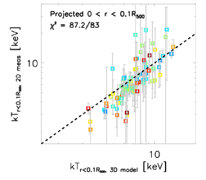
Refer to caption — Figure 1.— Comparison of 2-dimensional spectroscopic temperatures measured in an aperture of $r<0.1$ R₅₀₀ (with AGN masked) to the 3-dimensional model temperature projected onto the same annulus. The one-to-one correspondence (dashed line) between the data and models suggest that our mass-modeling approach (§2.4) yields reliable estimates of the central temperature for clusters that are relaxed. Point color corresponds to redshift, from $z=0.3$ (blue) to $z=1.2$ (red), indicating that the scatter in this plot is largely independent of redshift.

Based on this agreement, we feel confident extrapolating inwards into a regime without sufficient X-ray counts to measure the spectroscopic temperature and proceed throughout §3 utilizing the central ( $r<0.012$ R₅₀₀), deprojected model temperatures to calculate $t_{\textrm{cool},0}$ and K₀. In §4 we will return to the comparison between 2-D and 3-D quantities to determine the dependence of our results on this extrapolation and our choice of models.

3. Results

This sample represents the largest and most complete sample of galaxy clusters with X-ray observations at $z\gtrsim 0.4$ . Given the depth of our X-ray exposures, combined with the high angular resolution of the Chandra X-ray Observatory, we are in a unique position to study the evolution of cooling in the ICM for similar-mass clusters over timescales of $\sim$ 8 Gyr. In this section we will present the broad results of this study, drawing comparisons to samples of nearby clusters (e.g., White et al., 1997; Vikhlinin et al., 2006, 2009; Cavagnolo et al., 2009; Hudson et al., 2010). The interpretation of these results, as well as systematic errors that may affect them, are discussed in §4.

3.1. Cooling Time and Entropy Profiles

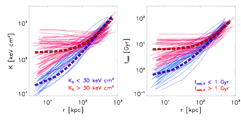
In Figure 2, we present the radial entropy and cooling time profiles for our full sample, based on the deprojection procedures described in §2.4. For comparison, we show the average entropy profiles for low-redshift cool core and non-cool core clusters from Cavagnolo et al. (2009). Perhaps surprisingly, there is no qualitative difference in the entropy profiles between this sample of high-redshift, massive, SZ-selected clusters and the low-redshift sample of groups and clusters presented in Cavagnolo et al. (2009).

Naively, one might expect the mean central entropy to decrease with time, as clusters have had more time to cool. However, the similarity between low-redshift clusters and this sample, which has a median redshift of 0.63 and a median age nearly half of the $z\sim 0$ sample, indicates that the entropy and cooling time profiles are unchanging. This suggests that the characteristic entropy and cooling time profiles, having minimal core entropies of $\sim$ 10 keV cm² and cooling radii of $\sim$ 100 kpc, were established at earlier times than we are probing with this sample ( $z\gtrsim 1$ ).

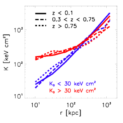
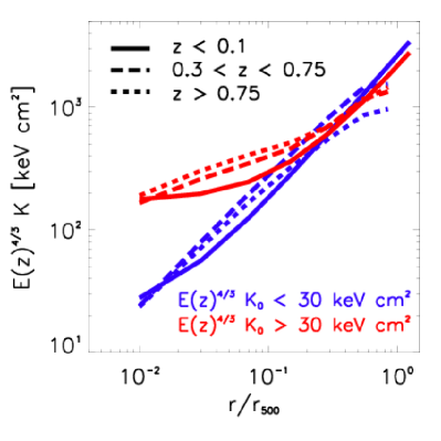
In order to look for evolution in the entropy profile, we plot in Figure 3 the average entropy profile for cool core (K ${}_{0}<30$ keV cm²) and non-cool core (K ${}_{0}>30$ keV cm²) clusters in the SPT-XVP sample, divided into two redshift bins corresponding to $z<0.75$ and $z>0.75$ . These are compared to the average profiles from Cavagnolo et al. (2009), for clusters at $z\lesssim 0.1$ . In general, the average profiles are indistinguishable in the inner few hundred kiloparsecs, with high-redshift clusters having slightly higher entropy at small radii ( $r\lesssim 200$ kpc) than their low-redshift counterparts. At larger radii, the profiles vary according to the self-similar E $(z)^{4/3}$ scaling (Pratt et al., 2010). These results suggest that the outer entropy profile is following the gravitational collapse of the cluster, while the inner profile has some additional physics governing its evolution, most likely baryonic cooling. The mild central entropy evolution in the right panel of Figure 3 could be thought of as the effect of “forcing” an evolutionary scaling in a regime where the profile is unevolving

The combination of Figures 2 and 3 suggests that the cooling properties of the intracluster medium in the inner $\sim$ 200 kpc have remained relatively constant over timescales of $\sim$ 8 Gyr. The short cooling times at these radii imply that the core entropy profile should change on short timescales. The fact that this is not observed suggests that some form of feedback has offset cooling on these exceptionally long timescales, keeping the central entropy at a constant value. There is evidence that mechanical feedback from AGN is stable over such long periods of time (Hlavacek-Larrondo et al., 2012), perhaps maintaining the observed entropy floor of 10 keV cm² since $z\sim 1.2$ .

3.2. Distribution of Central Entropy, Cooling Time, and Cooling Rate

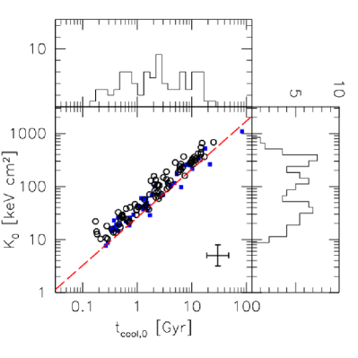
In Figure 4, we compare the derived central entropy and cooling time (see §2.4 for details on deriving central quantities) for the SPT-XVP sample to those for the low-redshift clusters in the Chandra Cluster Cosmology Project (hereafter CCCP; Vikhlinin et al., 2006, 2009). Overall, we find excellent agreement between the two samples. While it is unsurprising that these two quantities are correlated, due to their similar dependence on both T_X and n_e, the normalization and distribution of points along the sequence is reassuring. Both the SPT-XVP and the CCCP clusters have a slightly higher normalization than found by Hudson et al. (2010), which can be accounted for by the fact that both of these samples target more massive clusters. Indeed, Hudson et al. (2010) showed that the scatter about the $t_{\textrm{cool},0}$ –K₀ correlates with the cluster temperature, with high-T_X clusters lying above the relation and low-T_X groups lying below the relation. Similar to previous low-redshift studies (e.g., Cavagnolo et al., 2009; Hudson et al., 2010), we see hints of multiple peaks in both $t_{\textrm{cool},0}$ and K₀, with minima at $\sim$ 1 Gyr and 50 keV cm², respectively (e.g., Cavagnolo et al., 2009; Hudson et al., 2010). This threshold, separating cool core from non-cool core clusters, appears to be unchanged between the low-redshift and high-redshift samples. We will return to this point in §3.3.

In Figure 5, we plot the distribution of mass deposition rates, $d$ M $/dt$ , for our SPT-selected sample. We show the integrated cooling rate within two radii: $r$ ( $t_{\textrm{cool}}=t_{\textrm{Univ}})$ and $r(t_{\textrm{cool}}=7.7$ Gyr). The former is more physically motivated, representing the amount of gas that has had time to cool since the cluster formed. The latter is motivated by the desire to have the definition of the cooling radius be independent of redshift – the choice of a 7.7 Gyr timescale is arbitrary and was chosen simply to conform with the literature (e.g., O’Dea et al., 2008).

We find that clusters at high- $z$ have overall smaller time-averaged cooling rates, which is unsurprising given that they have had less time to cool. If we remove this factor by instead computing the cooling rate within a non-evolving aperture ( $r[t_{\textrm{cool}}=7.7$ Gyr]), we find no significant difference between the mass deposition rates measured in intermediate redshift ( $0.4<z<0.75$ ) and high redshift ( $0.75<z<1.1$ ) clusters. These sub-samples have median mass deposition rates of 49 M_⊙ yr^-1 and 57 M_⊙ yr^-1 (excluding non-cooling systems), respectively. For comparison, we also show the distribution of cooling rates for nearby clusters from White et al. (1997), for which the distribution is cut off at $d$ M $/dt$ $\lesssim$ 50 M_⊙ yr^-1 due to poorer sampling and, thus, reduced sensitivity to modest cooling rates. However, as evidenced by the cumulative distribution, at $d$ M $/dt$ $>$ 50 M_⊙ yr^-1 the three samples are nearly identical, suggesting very little evolution in the rate of cooling in the ICM over timescales of $\sim$ 8 Gyr.

3.3. Evolution of Cooling Flow Properties

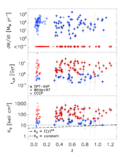
Figures 3 and 5 suggest that the cooling properties of the ICM vary little from $z\sim 0$ to $z\sim 1$ . In order to directly quantify this, we show in Figure 6 the evolution of $d$ M $/dt$ , K₀, and $t_{\textrm{cool},0}$ with redshift. For each quantity, we separate cool core and non-cool core clusters using the following thresholds: dM/dt $>0$ M_⊙ yr^-1, K ${}_{0}<30$ keV cm², and $t_{\textrm{cool},0}<1$ Gyr. This figure more clearly shows that there is very little, if any, evolution in the cooling properties of SPT-selected clusters over the range $0.3<z<1.2$ . We compare the range of $d$ M $/dt$ , K₀, and t_c,0 observed for these clusters to samples of nearby clusters from White et al. (1997) and the CCCP and find no appreciable change. The entropy floor, at K ${}_{0}\sim 10$ keV cm², is constant over the full redshift range of our sample, consistent with earlier work by Cavagnolo et al. (2009) which covered clusters at $0<z\lesssim 0.5$ . The data are also consistent with the self-similar expectation ( $E(z)^{4/3}$ ; Pratt et al., 2010), which predicts only a factor of $\sim$ 1.6 change in central entropy from $z=1$ to $z=0$ . This self-similar evolution is based on gravity alone – the fact that it is an adequate representation of the data in the central $\sim$ 100 kpc of clusters, where cooling processes should be responsible for shaping the entropy profile, suggests that cooling is offset exceptionally well over very long over the past $\sim$ 7 Gyr. In the absence of feedback, cool core clusters at $z\sim$ 1 should have $K_{0}\rightarrow 0$ in $<$ 1 Gyr.

3.4. Evolution of Cluster Surface Brightness Profiles

Figures 2–6 suggest that there is little change in the ICM cooling properties in the cores of X-ray- and SZ-selected clusters since $z\sim 1.2$ , in agreement with earlier studies at lower redshift (e.g., Cavagnolo et al., 2009). However, Several recent studies have argued that there are fewer cool core clusters at high redshift (Vikhlinin et al., 2007; Santos et al., 2008, 2010) based on measurements of surface brightness concentration, suggesting that “cool cores” and “cooling flows” may not have the same evolution and, thus, are not necessarily coupled at high redshift as they are now.

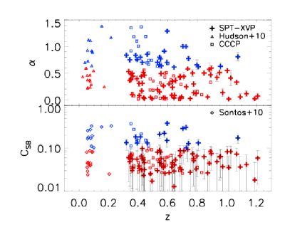
In Figure 7, we duplicate the analyses of Vikhlinin et al. (2007), Santos et al. (2008), and Semler et al. (2012) in order to look for evolution in the cool core properties. We find that the number of galaxy clusters classified as “cool core” by both $\alpha$ and $c_{SB}$ (see §2.3) decreases with redshift, from $\sim$ 40% at $z\sim 0$ to $\sim$ 10% at $z\gtrsim 0.75$ . These results confirm the evolution in cool core strength reported by Vikhlinin et al. (2007) and Santos et al. (2008) for X-ray selected samples, however the evolution appears to be a bit slower for the SZ-selected sample, with several strong cool cores in the range $0.5<z<0.75$ (Semler et al., 2012). The higher fraction of “moderate” cool cores in Figure 7 at higher redshift in consistent with recent work by Santos et al. (2010). All samples agree that there is a lack of strong, classical cool cores at $z>0.75$ , which seems to be in opposition to the results presented in Figures 2–6 which suggest no evolution in the cooling properties. One possible explanation for this discrepancy is that both the concentration parameter, $c_{SB}$ , and the cuspiness parameter, $\alpha$ , (see eqs. 3 & 4) assume no evolution in the scale radius of the cool core: $c_{SB}$ assumes a radius of 40 kpc, while $\alpha$ uses $0.04$ R₅₀₀.

To further investigate the surface brightness evolution, we move away from single-parameter measures of surface brightness concentration and, instead, directly compare the X-ray surface brightness profiles for low- and high-redshift clusters in Figure 8. At $z<0.75$ , we confirm that, overall, clusters with low central entropy (K ${}_{0}<30$ keV cm²) have more centrally-concentrated surface brightness profiles than those with high central entropy (K ${}_{0}>30$ keV cm²). However, at high redshift ( $z>0.75$ ) we find a lack of strongly-concentrated clusters, with only a weak increase in concentration for the clusters with low central entropy, consistent with earlier studies of distant X-ray-selected clusters (e.g., Vikhlinin et al., 2007; Santos et al., 2008, 2010). This difference in surface brightness concentration is not a result of increased spatial resolution for low-redshift clusters – the difference in spatial resolution between the centers of these redshift bins is only $\sim$ 30%.

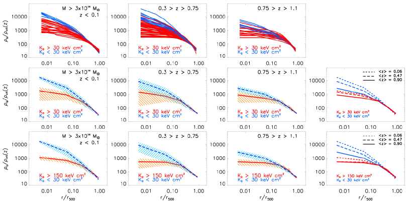This result becomes even more dramatic when the data are deprojected into gas density, rather than surface brightness, and including $z\sim 0$ clusters for comparison. In Figure 9, we compare the ICM gas density profiles for the sample presented in this work to a low-redshift sample (Chandra Cluster Cosmology Project; Vikhlinin et al., 2009). We restrict the low-redshift sample to clusters with M ${}_{500}>3\times 10^{14}$ M_⊙, in order to approximate the SPT-selection cut. This comparison is particularly appropriate since our reduction and analysis pipeline is identical to that used by Vikhlinin et al. (2009). Figure 9 shows that the 3-dimensional gas density profiles become more centrally concentrated with decreasing redshift, with nearly an order of magnitude difference in central gas density between cool core clusters at $z\sim 0.1$ and $z\sim 0.9$ . On the contrary, non-cooling clusters (K ${}_{0}>30$ keV cm²) experience no appreciable evolution in the central physical density over the same timescale. The combination of Figures 8 and 9 seem to suggest that the dense cores which are associated with cooling flows have built up slowly over the past $\sim$ 8 Gyr. This scenario would explain the lack of centrally-concentrated, or “cuspy”, clusters at high redshift.

4. Discussion

Figures 2–9 present an interesting story. The cooling properties of the intracluster medium in the most massive galaxy clusters appear to be relatively constant – that is, classical cooling rates are not getting any higher and central entropies are not getting any lower – since $z\sim 1.2$ . Over the same timescale, the central gas density has increased by roughly an order of magnitude in clusters exhibiting cooling signatures, leading to considerably more concentrated surface brightness profiles in low-redshift cool core clusters. Below, we discuss potential explanations for these results, along with systematics that may be confusing the issue.

4.1. The Origin of Cool Cores

The results presented thus far suggest that the dense cores associated with cooling flow clusters were not as pronounced $\sim$ 8 Gyr ago, despite the fact that clusters at these early times had similar cooling rates and central entropy (Figure 6). We propose that these cores have grown over time as a direct result of cooling flows being halted by feedback. In this scenario, gas from larger radii cools and flows inwards, but it hits a “cooling floor” at $\sim$ 10 keV cm², below which cooling is less efficient. This floor is likely a result of some form of feedback, with the most promising explanation currently being mechanical energy injection from the central AGN (e.g., Fabian, 2012; McNamara & Nulsen, 2012). This concept of a cooling floor is supported by observations. Peterson & Fabian (2006) show, using high resolution X-ray spectroscopy of nearby galaxy clusters, that gas at temperatures less than $\sim$ 1/3 of the ambient ICM temperature is cooling orders of magnitude less effectively than predicted. Further, in agreement with Cavagnolo et al. (2009), we show in Figure 6 that there is a lower entropy limit in the cores of galaxy clusters of $\sim$ 10 keV cm² which is roughly constant over the range $0<z<1.2$ . The fact that the ICM appears unable to cool efficiently below $\sim$ 1/3 of the ambient temperature, or $\sim$ 10 keV cm², implies that, if material is indeed flowing into the cluster core, then we should observe a build up of low-entropy gas in the core.

To test this hypothesis, we measure the “cool core mass” for all clusters in our sample with K ${}_{0}<30$ keV cm². The cool core mass is defined as:

\textrm{M}_{cool}=4\pi\int_{0}^{0.1\textrm{R}_{500}}(\rho_{g}-\left<\rho_{g,\textrm{NCC}}\right>)r^{2}dr,

(10)

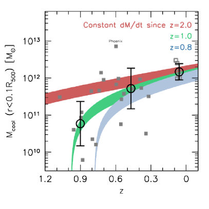
where $\left<\rho_{g,\textrm{NCC}}\right>$ represents the median non-cool core (K ${}_{0}>150$ keV cm²) density profile (Figure 9) and the outer radius of 0.1R₅₀₀ is roughly where the uncertainty in $\rho_{g}$ is similar in scale to the difference between the median cool core and non-cool core profiles. In Figure 10, we plot the cool core mass, M_cool, versus redshift for the full sample of SPT-XVP clusters with K ${}_{0}<30$ keV cm², including 5 nearby ( $z<0.1$ ) clusters from Vikhlinin et al. (2006). We find a rapid evolution in the total cool core mass, with an order of magnitude increase in M_cool between $z\sim 1$ and $z\sim 0.5$ . As we show in Figure 10, the median growth is fully consistent with a constant cooling flow since $z=1$ with $d$ M $/dt$ = 150 M_⊙ yr^-1. The range of cool core masses is consistent with cooing flowing initiating at $0.8\lesssim z\lesssim 2$ , providing the first constraints on the onset of cooling in galaxy clusters.

Figure 10 suggests that cool cores at $z\sim 0$ are a direct result of long-standing cooling flows (Figure 5) coupled with a constant entropy floor (Figure 6) – most likely the result of AGN feedback. The long-standing balance between cooling and feedback prevents gas from cooling completely and, instead, leads to an accumulation of cool gas in the core of the cluster.

This simple evolutionary scenario, which we offer as an explanation for the increase in central gas density in clusters from $z\sim 1$ to $z\sim 0.5$ , is based on a sample of massive (M ${}_{500}>2\times 10^{14}$ M_⊙), rich galaxy clusters. While the cooling rate (dM/dt) is proportional to cluster mass (White et al., 1997), there is no evidence that the presence of a cool core is dependent on whether the host is a rich galaxy cluster or a poor group (McDonald et al., 2011a). Thus, if these trends hold at $z\gg 0.1$ , we would expect future surveys of low-mass, high-redshift clusters, via optical (e.g., LSST; Tyson, 2002) or X-ray (e.g., eRosita; Predehl et al., 2007) detection, to see a similar decline in the cuspiness of cool cores at high redshift. At this point, however, such an extrapolation to lower masses is purely speculative.

4.2. The Evolution of ICM Cooling

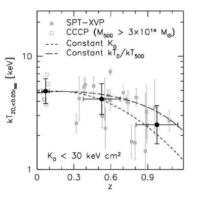
In Figure 6, we show that there is no measurable evolution in the minimum central entropy, K₀, over the range $0.3<z<1.2$ . Coupled with the apparent increase in central density, this would imply that cool cores today are warmer than their high- $z$ counterparts. Since a detailed spatial comparison, such as we did for density, is more challenging with a spectroscopically-measured quantity, we reduce the problem to a single measurement of “central” temperature. Here we define the central temperature as the spectroscopically-measured temperature within 0.05R₅₀₀, with central point sources masked. We consider here only systems with K ${}_{0}<30$ keV cm², which are the most centrally concentrated systems in our sample, allowing us to use a smaller aperture than in Figure 1.

In Figure 11, we see that, indeed, for clusters classified as cool core on the basis of their central entropy (K ${}_{0}<30$ keV cm²), central temperature increases with decreasing redshift. The slope of this relation is equally consistent with the expected self-similar evolution, as well as what is required to have no evolution in K₀ over this redshift interval (dashed line, see also Figure 6). This figure seems to suggest that there may be some additional heating in low-redshift cluster cores above the self-similar expectation, perhaps resulting from AGN feedback. However, we stress that these data are insufficient to distinguish between these two scenarios, and so we defer any further speculation on the evolution of the central temperature to an upcoming paper which will perform a careful stacking analysis of these clusters.

The combined evidence presented in §4.1 and §4.2 support the scenario that cooling material has been gradually building up in cluster cores over the last $\sim$ 8 Gyr, but has been prevented from completely cooling by an almost perfectly balanced heating source. While at first glance it would appear that the amount of energy injected by feedback must increase rapidly to offset increased cooling (L ${}_{\textrm{cool}}\propto n_{e}^{2}$ T^1/2), much of this is offset by the fact that the gravitational potential in the core is increasing, leading to more heating as cooling material falls into the potential well. So, while cool cores are becoming denser with decreasing redshift, the actual cooling rates, and by extension the energy needed for feedback to offset cooling, have remained nearly constant since $z\sim 1$ .

Recent observations of the “Phoenix Cluster” (McDonald et al., 2012b, 2013) suggest that some clusters may undergo episodes of runaway cooling, perhaps before the feedback responsible for establishing the cooling flow was fully established, or that the feedback mechanism is strongly episodic.

4.3. The Cool Core / Cooling Flow Fraction

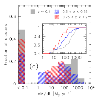
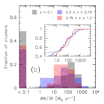
Much effort has recently focused on determining the fraction of high-redshift clusters which harbor a cool core (Vikhlinin et al., 2007; Santos et al., 2008, 2010; Samuele et al., 2011; McDonald, 2011; Semler et al., 2012). However, based on the results of this paper, we now know that the inferred evolution in the cool core fraction depends strongly on the criteria that are used to classify cool cores. In Figure 12 we demonstrate this point, showing that the measured fraction of high- $z$ cool cores is drastically different if the classification of cool cores is based on the presence of cooling (K₀, t ${}_{\textrm{cool},0}$ , $d$ M $/dt$ ; $\sim$ 35%) or cooled ( $\alpha$ , c_SB; $\sim$ 5%) gas. This figure shows that, at high redshift, it is important to differentiate between “cooling flows” and “cool cores” when classifying galaxy clusters as cooling or not – a distinction which is unnecessary in nearby clusters.

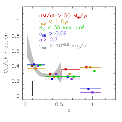
Figure 12 shows that the fraction of strongly-cooling clusters ( $d$ M $/dt>50$ M_⊙ yr^-1, K ${}_{0}<35$ keV cm², $t_{\textrm{cool},0}<1$ Gyr) undergoes little evolution over the range $0.3<z<1.2$ . This is qualitatively apparent in Figure 6. The fraction of strongly-cooling clusters increases from 25 ${}^{+11}_{-5}$ % to 35 ${}^{+10}_{-10}$ %, consistent at the $1\sigma$ level with no change. This figure shows that, not only is the rate at which the ICM is cooling roughly constant since $z\sim 1$ (Figure 5 and 6), but the fraction of clusters which experience strong cooling is also nearly constant over similar timescales.

It is also worth noting here the overall agreement in Figure 12 between the evolution of ICM cooling inferred from X-ray properties (this work) and optical properties (McDonald, 2011) at $z\leq 0.5$ . The latter sample was drawn from optically-selected catalogues, and used emission-line nebulae as a probe of ICM cooling. This overall agreement suggests that the evolution of cooling properties is relatively independent of how the clusters are selected (optical vs SZ). The steep rise in the cooling fraction at $z<0.5$ was interpreted by McDonald (2011) as being due to timing – we are seeing clusters transitioning from “weak” to “strong” cool cores as the central cooling time drops over time.

4.4. Potential Biases

While the observed cool core evolution presented here is interesting, it may suffer from a combination of several biases in both the sample selection and in the analysis. Below we address four biases and quantify their effects on the observed cool core evolution.

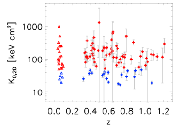
4.4.1 3-Dimensional Mass Modeling

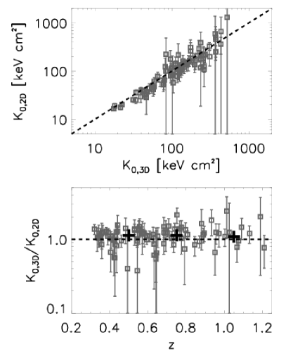
The results presented thus far rely on our ability to estimate the central temperature based on assumptions about the dark matter halo and hydrostatic equilibrium (see §2.3). While we established in §2.5 that these estimates are reliable, it is worthwhile to investigate whether any of the observed evolutionary trends are due to this approach. In Figure 13, we compare the central entropy calculated using a 2-dimensional, spectroscopically-measured temperature (see §2.5) to our 3-dimensional model calculation. We find very good one-to-one agreement between these two quantities, with the scatter being uncorrelated with redshift. This suggests that the observed lack of evolution in K₀ is not a result of our modeling technique. We further demonstrate this in Figure 14, showing the evolution of the central entropy based on the 2-dimensional central temperature. Comparing to low-redshift clusters from the CCCP, with K_0,2D calculated in the same way, we confirm the lack of evolution in the central entropy from Figure 6 over the range $0<z<1.2$ .

4.4.2 Increased SZ Signal in Cool Cores

In the central regions of cool core clusters, the increased density leads to a substantial increase in the inner pressure profile (Planck Collaboration et al., 2012). This should, in turn, lead to an increase in the SZ detection significance, biasing SZ-selected samples towards detecting clusters with dense cores. However, given the small relative volume and mass of cool cores to the rest of the cluster, we expect this bias to be small. This bias was first quantified via detailed numerical simulations by Motl et al. (2005). These authors found that integrated SZ quantities were relatively unbiased. In simulations that allowed unrestricted radiative cooling, the logarithmic slope, $\alpha$ , of the $M_{500}-y_{SZ}$ relation increased by $\sim$ 7.5% over their non-cooling counterparts. It is well understood that galaxy clusters which are simulated without feedback or star formation become too centrally concentrated (the “over-cooling problem”; Balogh et al., 2001), so this represents the upper limit of the SZ bias due to the presence of ICM cooling. When Motl et al. (2005) include star formation and stellar feedback – which yields the most realistic-looking cool core clusters – the difference in $\alpha$ between cooing and non-cooling clusters is reduced to $\sim$ 1%. The relatively small bias of SZ integrated quantities was confirmed by Pipino & Pierpaoli (2010), who explicitly simulated the bias for a SPT-like survey and found that, at masses above $\sim 2\times 10^{14}$ M_⊙, the observed fraction of non-cool cores with the SPT should be nearly identical to the true fraction. In an upcoming publication (Lin et al. in prep), we further show that this small bias is nearly redshift independent. Thus, while there is a small bias in the SZ signal due to the presence of a low-entropy core, we do not expect this bias to seriously alter our results, due both to its small magnitude and weak redshift dependence.

4.4.3 X-ray Centroid Determination

In §2.2 we describe our method of determining the cluster center, which is based on the X-ray emission in an annulus of 250–500 kpc. This method, which reduces scatter in X-ray scaling relations by finding the large-scale center rather than what may be the displaced core, will yield less centrally-concentrated density profiles than if we chose the X-ray peak as the cluster center. Regardless of how the center is defined, we can investigate how our choice can affect the resulting density profile.

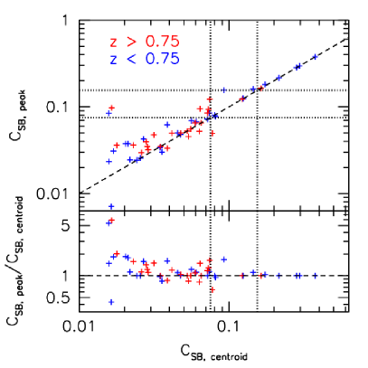
In Figure 15, we compare the measured surface brightness concentration (c_SB; Santos et al., 2008) based on our large-scale centroid and the X-ray peak. This figure confirms that, for relaxed strong cool cores, the X-ray peak and the large-scale centroid are nearly equivalent. By switching to c_SB,peak, the number of high- $z$ strong cool cores (c ${}_{SB}>0.155$ ) would remain constant at 1, while the number of low- $z$ strong cool cores would increase from 5 to 7. Repeating this exercise for moderate cool cores ( $0.075<c_{SB}<0.155$ ) we find increases of 5 (from 1 to 6) and 2 (from 3 to 5) for high and low redshift clusters, respectively. This large difference is primarily due to the arbitrary definition of moderate cool cores – if we switched to a threshold of 0.07 rather than 0.075, the number of high- $z$ clusters which would be re-classified as moderate cool cores by re-defining the center would decrease from 5 to 2. Perhaps most importantly, the increase in c_SB resulting from changing the center to the X-ray peak appears to have no dependence on redshift, as the lower panel of Figure 15 demonstrates. Thus, while the choice of center certainly affects the shape of the density profile, there is no evidence that this could result in low- $z$ clusters being measured to be more centrally concentrated than their high- $z$ counterparts.

4.4.4 Radio-Loud and Star-forming BCGs

There is a strong correlation in the local Universe between the presence of a cool core and radio emission from the BCG (Sun, 2009), which may conspire to fill in the SZ signal for the strongest cool cores. Intuitively, this bias should tend to be strongest for nearby clusters (since the SZ signal is nearly redshift independent, but radio flux is not), which would lead to a bias against detecting strong cool cores at low redshift with the SZ effect. This is exactly the opposite of what we observe – the strongest cool cores in our sample are all at $z<0.75$ , with a general lack of such systems at high redshift. We can further quantify this bias by appealing to Figure 3 from Sayers et al. (2013), which presents a correlation between radio flux density and the SZ bias for Bolocam, which has a similar frequency coverage to SPT. This figure demonstrates that a 140 GHz flux density of $>$ 0.5 mJy is required to produce more than a 1% change in the SZ S/N measurement. Assuming a typical radio luminosity for strong cool cores of 10³² erg s^-1 Hz^-1 (Sun, 2009), and a spectral index of $\alpha=-0.8$ , we find a typical 140 GHz flux at $z=0.3$ of 0.9 mJy, corresponding to an SZ bias of $\sim 3$ %. While there certainly may be systems with higher radio luminosity in this sample, we note that this bias becomes substantially weaker with increasing redshift. This conclusion qualitatively agrees with estimates from radio observations of clusters which found that correlated radio emission is negligible relative to the SZ signal at 150 GHz for typical clusters in the SPT mass and redshift range (Lin et al., 2009; Sehgal et al., 2010) Thus, we conclude that radio-loud BCGs should not substantially bias our sample against cool core clusters, and certainly can not drive the observed growth of cool cores that we observe.

The most star-forming BCG in this sample is in the Phoenix cluster (SPT-CLJ2344-4243; McDonald et al., 2012b, 2013), with a star formation rate of $\sim$ 800 M_⊙ yr^-1. In McDonald et al. (2012b) we demonstrated that, at 1.5mm and 2.0mm, the flux of this source would be $\sim$ 0.5 mJy and $\sim$ 0.1 mJy, respectively. This is significantly lower than the detection limit of the SPT ( $\sim$ 20 mJy), suggesting that star formation has a negligible effect on the SZ signal. Since the other 82 clusters in this sample have significantly lower star formation rates, we conclude that star-forming BCGs are not biasing our selection for or against cool cores.

4.4.5 X-ray Underluminous Clusters

If there is a population of galaxy clusters at high-z which meet our mass threshold (M ${}_{500}>2\times 10^{14}$ M_⊙) but are gas-poor ( $f_{gas}\ll 0.125$ ) and, as a result, go undetected in the SPT survey, then our estimate of the cool core fraction (e.g., Figure 12) would be biased high. Such “X-ray underluminous” clusters have been identified in large optical surveys, and may be the result of either delayed assembly of the ICM or strong interactions that strip a substantial fraction of the hot gas. However, these systems are, in general, lower mass than the clusters which we consider here. Indeed, Koester et al. (2007) show, using a sample of 13,823 optically-selected galaxy clusters, that there is a near 1-to-1 correspondence between optically-selected and X-ray selected clusters at the high mass end, with the fraction of X-ray underluminous clusters increasing with decreasing cluster richness. Thus, assuming we can extrapolate this to high redshift, we do not expect that our results are seriously biased by the presence of a significant population of massive, high-redshift, gas-poor galaxy clusters.

5. Summary

We present X-ray observations of 83 massive SZ-selected clusters from the 2500 deg² South Pole Telescope SZ (SPT-SZ) survey, which includes the first results of a large Chandra X-ray Observatory program to observe the 80 most-significant clusters detected at $z>0.4$ from the first 2000 deg² of the SPT-SZ survey. This uniformly-selected sample provides a unique opportunity to study the evolution of the cooling intracluster medium in clusters from $z=0.3$ to $z=1.2$ .

We find no evolution in the cooling properties of the intracluster medium over this large redshift range, with the average entropy and cooling time profiles remaining roughly constant in the inner $\sim$ 100 kpc despite the outer profile ( $r>200$ kpc) following self-similar evolution. The distribution of the central entropy (K₀), central cooling time ( $t_{cool,0}$ ), and mass deposition rate ( $d$ M $/dt$ ) in cool core clusters remains unchanged from $z=0$ to $z=1.2$ . Further, the fraction of clusters experiencing strong cooling ( $\sim$ 30%) has not changed significantly over the 8 Gyr sampled here. The fact that the cooling properties of galaxy clusters are not evolving suggests that feedback is balancing cooling on very long ( $\sim$ 8 Gyr) timescales.

We observe a strong evolution in the central density of galaxy clusters over this same timescale, with the average $\rho_{g,0}$ / $\rho_{crit}$ increasing by a factor of $\sim$ 10 in this same redshift interval. We find a general lack of centrally concentrated cool cores at $z>0.75$ , consistent with earlier reports of a lack of cool cores at high redshift from X-ray surveys. We show that this steady growth of cool cores from $z>1$ to $z=0$ is consistent with a cooling flow of $\sim$ 150 M_⊙ yr^-1 which is unable to reach entropies below 10 keV cm², leading to an accumulation of cool gas in the central $\sim$ 100 kpc. In order to build cool cores of the observed masses at $z\sim 0$ , we estimate that cooling flows would need to begin at $0.8<z<2.0$ in most massive galaxy clusters. This work represents the first observations of galaxy clusters that span a broad enough redshift range and are sufficiently well-selected to track the growth of cool cores from their formation. These measurements give further evidence that stable, long-standing feedback is required to both halt cooling of the ICM to low temperatures and grow cool, dense cores.

This dataset, which contains dozens of new clusters, both cooling and non-cooling, at $0.3<z<1.2$ will prove invaluable for understanding the complex interplay between cooling and feedback in galaxy cluster cores, the formation and evolution of galaxy clusters, and the growth of massive central galaxies in cluster cores.

Acknowledgements

M. M. acknowledges support by NASA through a Hubble Fellowship grant HST-HF51308.01-A awarded by the Space Telescope Science Institute, which is operated by the Association of Universities for Research in Astronomy, Inc., for NASA, under contract NAS 5-26555. The South Pole Telescope program is supported by the National Science Foundation through grant ANT-0638937. Partial support is also provided by the NSF Physics Frontier Center grant PHY-0114422 to the Kavli Institute of Cosmological Physics at the University of Chicago, the Kavli Foundation, and the Gordon and Betty Moore Foundation. Support for X-ray analysis was provided by NASA through Chandra Award Numbers 12800071, 12800088, and 13800883 issued by the Chandra X-ray Observatory Center, which is operated by the Smithsonian Astrophysical Observatory for and on behalf of NASA. Galaxy cluster research at Harvard is supported by NSF grant AST-1009012 and at SAO in part by NSF grants AST-1009649 and MRI-0723073. Argonne National Laboratory’s work was supported under U.S. Department of Energy contract DE-AC02-06CH11357.

References

Allen (2000) Allen, S. W. 2000, MNRAS, 315, 269
Andersson et al. (2011) Andersson, K., Benson, B. A., Ade, P. A. R., et al. 2011, ApJ, 738, 48
Arnaud (1996) Arnaud, K. A. 1996, in Astronomical Society of the Pacific Conference Series, Vol. 101, Astronomical Data Analysis Software and Systems V, ed. G. H. Jacoby & J. Barnes, 17–+
Balogh et al. (2001) Balogh, M. L., Pearce, F. R., Bower, R. G., & Kay, S. T. 2001, MNRAS, 326, 1228
Benson et al. (2013) Benson, B. A., de Haan, T., Dudley, J. P., et al. 2013, ApJ, 763, 147
Bregman et al. (2006) Bregman, J. N., Fabian, A. C., Miller, E. D., & Irwin, J. A. 2006, ApJ, 642, 746
Bregman et al. (2001) Bregman, J. N., Miller, E. D., & Irwin, J. A. 2001, ApJ, 553, L125
Brodwin et al. (2010) Brodwin, M., Ruel, J., Ade, P. A. R., et al. 2010, ApJ, 721, 90
Carlstrom et al. (2011) Carlstrom, J. E., Ade, P. A. R., Aird, K. A., et al. 2011, PASP, 123, 568
Cavagnolo et al. (2009) Cavagnolo, K. W., Donahue, M., Voit, G. M., & Sun, M. 2009, ApJS, 182, 12
Churazov et al. (2001) Churazov, E., Brüggen, M., Kaiser, C. R., Böhringer, H., & Forman, W. 2001, ApJ, 554, 261
Crawford et al. (1999) Crawford, C. S., Allen, S. W., Ebeling, H., Edge, A. C., & Fabian, A. C. 1999, MNRAS, 306, 857
Donahue et al. (2011) Donahue, M., de Messières, G. E., O’Connell, R. W., et al. 2011, ApJ, 732, 40
Donahue et al. (1992) Donahue, M., Stocke, J. T., & Gioia, I. M. 1992, ApJ, 385, 49
Donahue et al. (2010) Donahue, M., Bruch, S., Wang, E., et al. 2010, ApJ, 715, 881
Duffy et al. (2008) Duffy, A. R., Schaye, J., Kay, S. T., & Dalla Vecchia, C. 2008, MNRAS, 390, L64
Edge (2001) Edge, A. C. 2001, MNRAS, 328, 762
Edge & Frayer (2003) Edge, A. C., & Frayer, D. T. 2003, ApJ, 594, L13
Edge et al. (2010) Edge, A. C., Oonk, J. B. R., Mittal, R., et al. 2010, A&A, 518, L46
Edwards et al. (2007) Edwards, L. O. V., Hudson, M. J., Balogh, M. L., & Smith, R. J. 2007, MNRAS, 379, 100
Fabian (1994) Fabian, A. C. 1994, ARA&A, 32, 277
Fabian (2012) —. 2012, ArXiv e-prints, arXiv:1204.4114
Foley et al. (2011) Foley, R. J., Andersson, K., Bazin, G., et al. 2011, ApJ, 731, 86
Gómez et al. (2002) Gómez, P. L., Loken, C., Roettiger, K., & Burns, J. O. 2002, ApJ, 569, 122
Hatch et al. (2007) Hatch, N. A., Crawford, C. S., & Fabian, A. C. 2007, MNRAS, 380, 33
Heckman et al. (1989) Heckman, T. M., Baum, S. A., van Breugel, W. J. M., & McCarthy, P. 1989, ApJ, 338, 48
Hicks et al. (2010) Hicks, A. K., Mushotzky, R., & Donahue, M. 2010, ApJ, 719, 1844
Hlavacek-Larrondo et al. (2012) Hlavacek-Larrondo, J., Fabian, A. C., Edge, A. C., et al. 2012, MNRAS, 421, 1360
Hu et al. (1985) Hu, E. M., Cowie, L. L., & Wang, Z. 1985, ApJS, 59, 447
Hudson et al. (2010) Hudson, D. S., Mittal, R., Reiprich, T. H., et al. 2010, A&A, 513, A37
Jaffe et al. (2005) Jaffe, W., Bremer, M. N., & Baker, K. 2005, MNRAS, 360, 748
Johnstone et al. (1987) Johnstone, R. M., Fabian, A. C., & Nulsen, P. E. J. 1987, MNRAS, 224, 75
Kalberla et al. (2005) Kalberla, P. M. W., Burton, W. B., Hartmann, D., et al. 2005, A&A, 440, 775
Koester et al. (2007) Koester, B. P., McKay, T. A., Annis, J., et al. 2007, ApJ, 660, 239
Lim et al. (2008) Lim, J., Ao, Y., & Dinh-V-Trung. 2008, ApJ, 672, 252
Lim et al. (2012) Lim, J., Ohyama, Y., Chi-Hung, Y., Dinh-V-Trung, & Shiang-Yu, W. 2012, ApJ, 744, 112
Lin et al. (2009) Lin, Y.-T., Partridge, B., Pober, J. C., et al. 2009, ApJ, 694, 992
Marriage et al. (2011) Marriage, T. A., Acquaviva, V., Ade, P. A. R., et al. 2011, ApJ, 737, 61
Mathews (2009) Mathews, W. G. 2009, ApJ, 695, L49
McDonald (2011) McDonald, M. 2011, ApJ, 742, L35
McDonald et al. (2013) McDonald, M., Benson, B., Veilleux, S., Bautz, M. W., & Reichardt, C. L. 2013, ApJ, 765, L37
McDonald et al. (2011a) McDonald, M., Veilleux, S., & Mushotzky, R. 2011a, ApJ, 731, 33
McDonald et al. (2010) McDonald, M., Veilleux, S., Rupke, D. S. N., & Mushotzky, R. 2010, ApJ, 721, 1262
McDonald et al. (2011b) McDonald, M., Veilleux, S., Rupke, D. S. N., Mushotzky, R., & Reynolds, C. 2011b, ApJ, 734, 95
McDonald et al. (2012a) McDonald, M., Wei, L. H., & Veilleux, S. 2012a, ApJ, 755, L24
McDonald et al. (2012b) McDonald, M., Bayliss, M., Benson, B. A., et al. 2012b, Nature, 488, 349
McNamara & Nulsen (2007) McNamara, B. R., & Nulsen, P. E. J. 2007, ARA&A, 45, 117
McNamara & Nulsen (2012) —. 2012, New Journal of Physics, 14, 055023
McNamara & O’Connell (1989) McNamara, B. R., & O’Connell, R. W. 1989, AJ, 98, 2018
Motl et al. (2005) Motl, P. M., Hallman, E. J., Burns, J. O., & Norman, M. L. 2005, ApJ, 623, L63
Nagai et al. (2007) Nagai, D., Kravtsov, A. V., & Vikhlinin, A. 2007, ApJ, 668, 1
Navarro et al. (1997) Navarro, J. F., Frenk, C. S., & White, S. D. M. 1997, ApJ, 490, 493
O’Dea et al. (2008) O’Dea, C. P., Baum, S. A., Privon, G., et al. 2008, ApJ, 681, 1035
Oegerle et al. (2001) Oegerle, W. R., Cowie, L., Davidsen, A., et al. 2001, ApJ, 560, 187
Peres et al. (1998) Peres, C. B., Fabian, A. C., Edge, A. C., et al. 1998, MNRAS, 298, 416
Peterson & Fabian (2006) Peterson, J. R., & Fabian, A. C. 2006, Phys. Rep., 427, 1
Pfrommer et al. (2012) Pfrommer, C., Chang, P., & Broderick, A. E. 2012, ApJ, 752, 24
Pipino & Pierpaoli (2010) Pipino, A., & Pierpaoli, E. 2010, MNRAS, 404, 1603
Planck Collaboration et al. (2011) Planck Collaboration, Aghanim, N., Arnaud, M., et al. 2011, A&A, 536, A10
Planck Collaboration et al. (2012) Planck Collaboration, Ade, P. A. R., Aghanim, N., et al. 2012, ArXiv e-prints, arXiv:1207.4061
Pratt et al. (2010) Pratt, G. W., Arnaud, M., Piffaretti, R., et al. 2010, A&A, 511, A85
Predehl et al. (2007) Predehl, P., Andritschke, R., Bornemann, W., et al. 2007, in Society of Photo-Optical Instrumentation Engineers (SPIE) Conference Series, Vol. 6686, Society of Photo-Optical Instrumentation Engineers (SPIE) Conference Series
Rafferty et al. (2008) Rafferty, D. A., McNamara, B. R., & Nulsen, P. E. J. 2008, ApJ, 687, 899
Reichardt et al. (2013) Reichardt, C. L., Stalder, B., Bleem, L. E., et al. 2013, ApJ, 763, 127
Russell et al. (2012) Russell, H. R., Fabian, A. C., Taylor, G. B., et al. 2012, MNRAS, 422, 590
Salomé & Combes (2003) Salomé, P., & Combes, F. 2003, A&A, 412, 657
Salomé et al. (2008) Salomé, P., Combes, F., Revaz, Y., et al. 2008, A&A, 484, 317
Samuele et al. (2011) Samuele, R., McNamara, B. R., Vikhlinin, A., & Mullis, C. R. 2011, ApJ, 731, 31
Sanders et al. (2010) Sanders, J. S., Fabian, A. C., Smith, R. K., & Peterson, J. R. 2010, MNRAS, 402, L11
Santos et al. (2008) Santos, J. S., Rosati, P., Tozzi, P., et al. 2008, A&A, 483, 35
Santos et al. (2010) Santos, J. S., Tozzi, P., Rosati, P., & Böhringer, H. 2010, A&A, 521, A64+
Santos et al. (2012) Santos, J. S., Tozzi, P., Rosati, P., Nonino, M., & Giovannini, G. 2012, A&A, 539, A105
Sayers et al. (2013) Sayers, J., Mroczkowski, T., Czakon, N. G., et al. 2013, ApJ, 764, 152
Sehgal et al. (2010) Sehgal, N., Bode, P., Das, S., et al. 2010, ApJ, 709, 920
Semler et al. (2012) Semler, D. R., Šuhada, R., Aird, K. A., et al. 2012, ArXiv e-prints, arXiv:1208.3368
Siemiginowska et al. (2010) Siemiginowska, A., Burke, D. J., Aldcroft, T. L., et al. 2010, ApJ, 722, 102
Song et al. (2012) Song, J., Zenteno, A., Stalder, B., et al. 2012, ArXiv e-prints, arXiv:1207.4369
Sparks et al. (2012) Sparks, W. B., Pringle, J. E., Carswell, R. F., et al. 2012, ApJ, 750, L5
Staniszewski et al. (2009) Staniszewski, Z., Ade, P. A. R., Aird, K. A., et al. 2009, ApJ, 701, 32
Sun (2009) Sun, M. 2009, ApJ, 704, 1586
Sun et al. (2009) Sun, M., Voit, G. M., Donahue, M., et al. 2009, ApJ, 693, 1142
Sunyaev & Zeldovich (1972) Sunyaev, R. A., & Zeldovich, Y. B. 1972, Comments on Astrophysics and Space Physics, 4, 173
Sutherland & Dopita (1993) Sutherland, R. S., & Dopita, M. A. 1993, ApJS, 88, 253
Tyson (2002) Tyson, J. A. 2002, in Society of Photo-Optical Instrumentation Engineers (SPIE) Conference Series, Vol. 4836, Society of Photo-Optical Instrumentation Engineers (SPIE) Conference Series, ed. J. A. Tyson & S. Wolff, 10–20
Vanderlinde et al. (2010) Vanderlinde, K., Crawford, T. M., de Haan, T., et al. 2010, ApJ, 722, 1180
Vikhlinin et al. (2007) Vikhlinin, A., Burenin, R., Forman, W. R., et al. 2007, in Heating versus Cooling in Galaxies and Clusters of Galaxies, ed. H. Böhringer, G. W. Pratt, A. Finoguenov, & P. Schuecker , 48–+
Vikhlinin et al. (2006) Vikhlinin, A., Kravtsov, A., Forman, W., et al. 2006, ApJ, 640, 691
Vikhlinin et al. (2005) Vikhlinin, A., Markevitch, M., Murray, S. S., et al. 2005, ApJ, 628, 655
Vikhlinin et al. (1998) Vikhlinin, A., McNamara, B. R., Forman, W., et al. 1998, ApJ, 498, L21
Vikhlinin et al. (2009) Vikhlinin, A., Burenin, R. A., Ebeling, H., et al. 2009, ApJ, 692, 1033
White et al. (1997) White, D. A., Jones, C., & Forman, W. 1997, MNRAS, 292, 419
Williamson et al. (2011) Williamson, R., Benson, B. A., High, F. W., et al. 2011, ApJ, 738, 139
Wyithe et al. (2001) Wyithe, J. S. B., Turner, E. L., & Spergel, D. N. 2001, ApJ, 555, 504
Zhao (1996) Zhao, H. 1996, MNRAS, 278, 488

Appendix A Temperature and Density Profiles – Data and Models

Below, we show the X-ray data for all 83 clusters presented in this work. For each cluster, we show a smoothed X-ray image (0.5–5.0 keV), a surface brightness profile (§2.3), and a 3-bin projected temperature profile (§2.4). On both the surface brightness and temperature profiles, we overlay (gray curve) the best-fit models from our mass-modeling technique (§2.4). These images demonstrate the ability of our algorithm to accurately predict the central temperature given only a coarse temperature profile combined with a well-sampled gas density profile and assumptions about the dark matter halo. With few exceptions, this technique provides an excellent fit to the projected temperature profiles, regardless of whether the cluster is relaxed (e.g., SPT-CLJ2344-4243) or disturbed (e.g., SPT-CLJ0542-4100).

Appendix B Cool Core / Cooling Flow Properties

Below we provide cool core and cooling flow properties for the full sample of 83 galaxy clusters at $0.3<z<1.2$ . A complete description of how these values were measured is presented in §2. As in §2–§4, we use the subscript “0” to represent the measured quantity in our smallest annulus: $r<0.012{\rm R}_{500}$ . All of these data are deprojected, using our mass-modeling technique described in §3.

(1)	(2)	(3)	(4)	(5)	(6)	(7)	(8)	(9)
Cluster Name	$n_{e,0}$	kT₀	c_SB	$\alpha$	K₀	$t_{\textrm{cool},0}$	$d$ M $/dt_{7.7}$	$d$ M $/dt_{\textrm{Univ}}$
	[cm^-3]	[keV]			[keV cm²]	[Gyr]	[M_⊙ yr^-1]	[M_⊙ yr^-1]
SPT-CLJ0000-5748	0.164 ${}^{+0.004}_{-0.004}$	4.2 $\pm$ 0.6	0.29 ${}^{+0.03}_{-0.04}$	1.00 $\pm$ 0.04	14.1 ${}^{+2.2}_{-2.1}$	0.18 ${}^{+0.03}_{-0.03}$	437.3 ${}^{+68.1}_{-51.9}$	437.3 ${}^{+68.1}_{-51.9}$
SPT-CLJ0013-4906	0.007 ${}^{+0.000}_{-0.000}$	8.0 $\pm$ 1.6	0.03 ${}^{+0.00}_{-0.02}$	0.09 $\pm$ 0.01	229.8 ${}^{+50.9}_{-49.5}$	6.83 ${}^{+1.57}_{-1.51}$	–	33.3 ${}^{+8.5}_{-5.6}$
SPT-CLJ0014-4952	0.004 ${}^{+0.000}_{-0.000}$	7.4 $\pm$ 0.9	0.03 ${}^{+0.00}_{-0.01}$	0.03 $\pm$ 0.00	309.6 ${}^{+42.1}_{-41.2}$	11.44 ${}^{+1.63}_{-1.58}$	–	–
SPT-CLJ0033-6326	0.042 ${}^{+0.002}_{-0.002}$	2.3 $\pm$ 1.4	0.08 ${}^{+0.01}_{-0.03}$	0.77 $\pm$ 0.06	19.2 ${}^{+12.4}_{-11.8}$	0.47 ${}^{+0.31}_{-0.29}$	57.1 ${}^{+87.8}_{-21.5}$	83.1 ${}^{+127.8}_{-31.4}$
SPT-CLJ0037-5047	0.009 ${}^{+0.001}_{-0.001}$	5.1 $\pm$ 7.3	0.08 ${}^{+0.03}_{-0.04}$	0.41 $\pm$ 0.14	115.7 ${}^{+183.8}_{-161.9}$	3.67 ${}^{+6.13}_{-5.08}$	0.0 ${}^{+-0.0}_{-0.0}$	0.0 ${}^{+-0.0}_{-0.0}$
SPT-CLJ0040-4407	0.018 ${}^{+0.000}_{-0.000}$	7.5 $\pm$ 1.9	0.07 ${}^{+0.00}_{-0.02}$	0.38 $\pm$ 0.04	108.0 ${}^{+29.9}_{-28.9}$	2.34 ${}^{+0.67}_{-0.64}$	86.2 ${}^{+29.6}_{-17.6}$	159.8 ${}^{+54.9}_{-32.5}$
SPT-CLJ0058-6145	0.031 ${}^{+0.001}_{-0.001}$	2.4 $\pm$ 1.7	0.06 ${}^{+0.00}_{-0.02}$	0.63 $\pm$ 0.06	24.0 ${}^{+18.5}_{-17.8}$	0.64 ${}^{+0.51}_{-0.48}$	25.4 ${}^{+70.3}_{-10.8}$	15.2 ${}^{+42.1}_{-6.4}$
SPT-CLJ0102-4603	0.025 ${}^{+0.001}_{-0.001}$	0.9 $\pm$ 0.5	0.07 ${}^{+0.01}_{-0.02}$	0.66 $\pm$ 0.09	10.3 ${}^{+6.1}_{-5.8}$	0.29 ${}^{+0.18}_{-0.16}$	58.7 ${}^{+74.1}_{-21.0}$	58.7 ${}^{+74.1}_{-21.0}$
SPT-CLJ0102-4915	0.009 ${}^{+0.000}_{-0.000}$	16.2 $\pm$ 2.3	0.03 ${}^{+0.01}_{-0.01}$	0.06 $\pm$ 0.00	364.6 ${}^{+54.5}_{-53.8}$	7.10 ${}^{+1.09}_{-1.07}$	–	–
SPT-CLJ0123-4821	0.004 ${}^{+0.000}_{-0.000}$	7.3 $\pm$ 1.5	0.04 ${}^{+0.00}_{-0.02}$	0.09 $\pm$ 0.04	276.3 ${}^{+61.9}_{-60.1}$	9.77 ${}^{+2.28}_{-2.18}$	–	–
SPT-CLJ0142-5032	0.005 ${}^{+0.000}_{-0.000}$	8.5 $\pm$ 1.7	0.03 ${}^{+0.00}_{-0.02}$	0.06 $\pm$ 0.01	307.7 ${}^{+70.5}_{-67.7}$	10.03 ${}^{+2.43}_{-2.29}$	–	–
SPT-CLJ0151-5954	0.004 ${}^{+0.000}_{-0.000}$	6.2 $\pm$ 2.8	0.04 ${}^{+0.00}_{-0.02}$	0.02 $\pm$ 0.02	264.9 ${}^{+130.5}_{-123.3}$	10.62 ${}^{+5.46}_{-5.02}$	–	–
SPT-CLJ0156-5541	0.008 ${}^{+0.000}_{-0.000}$	9.7 $\pm$ 2.5	0.06 ${}^{+0.00}_{-0.02}$	0.07 $\pm$ 0.06	238.6 ${}^{+70.9}_{-66.9}$	6.06 ${}^{+1.92}_{-1.76}$	–	–
SPT-CLJ0200-4852	0.017 ${}^{+0.000}_{-0.000}$	7.0 $\pm$ 3.0	0.05 ${}^{+0.00}_{-0.02}$	0.52 $\pm$ 0.05	105.5 ${}^{+48.6}_{-47.0}$	2.42 ${}^{+1.14}_{-1.09}$	–	2.4 ${}^{+1.9}_{-0.7}$
SPT-CLJ0212-4657	0.004 ${}^{+0.000}_{-0.000}$	8.2 $\pm$ 2.4	0.04 ${}^{+0.00}_{-0.02}$	0.04 $\pm$ 0.01	340.7 ${}^{+108.6}_{-104.5}$	12.14 ${}^{+4.03}_{-3.81}$	–	–
SPT-CLJ0217-5245	0.019 ${}^{+0.000}_{-0.000}$	1.6 $\pm$ 1.5	0.06 ${}^{+0.00}_{-0.02}$	0.75 $\pm$ 0.04	21.8 ${}^{+21.3}_{-20.7}$	0.73 ${}^{+0.72}_{-0.69}$	5.8 ${}^{+100.7}_{-2.8}$	5.8 ${}^{+100.7}_{-2.8}$
SPT-CLJ0232-5257	0.020 ${}^{+0.001}_{-0.001}$	1.6 $\pm$ 0.8	0.04 ${}^{+0.00}_{-0.02}$	0.64 $\pm$ 0.05	21.3 ${}^{+12.2}_{-11.6}$	0.70 ${}^{+0.41}_{-0.38}$	40.4 ${}^{+46.6}_{-14.1}$	40.4 ${}^{+46.6}_{-14.1}$
SPT-CLJ0234-5831	0.058 ${}^{+0.001}_{-0.001}$	5.7 $\pm$ 0.6	0.18 ${}^{+0.01}_{-0.03}$	0.80 $\pm$ 0.05	38.1 ${}^{+4.4}_{-4.3}$	0.63 ${}^{+0.08}_{-0.08}$	427.8 ${}^{+46.7}_{-38.4}$	427.8 ${}^{+46.7}_{-38.4}$
SPT-CLJ0236-4938	0.011 ${}^{+0.000}_{-0.000}$	3.1 $\pm$ 1.7	0.06 ${}^{+0.00}_{-0.02}$	0.54 $\pm$ 0.04	61.8 ${}^{+35.9}_{-35.0}$	2.20 ${}^{+1.30}_{-1.25}$	2.2 ${}^{+2.8}_{-0.8}$	2.2 ${}^{+2.8}_{-0.8}$
SPT-CLJ0243-5930	0.015 ${}^{+0.000}_{-0.000}$	6.4 $\pm$ 1.9	0.05 ${}^{+0.00}_{-0.02}$	0.35 $\pm$ 0.05	104.3 ${}^{+31.9}_{-31.1}$	2.55 ${}^{+0.80}_{-0.77}$	15.2 ${}^{+6.2}_{-3.4}$	15.2 ${}^{+6.2}_{-3.4}$
SPT-CLJ0252-4824	0.008 ${}^{+0.000}_{-0.000}$	2.3 $\pm$ 1.0	0.03 ${}^{+0.00}_{-0.02}$	0.44 $\pm$ 0.06	58.6 ${}^{+26.5}_{-25.7}$	2.47 ${}^{+1.15}_{-1.09}$	2.3 ${}^{+1.7}_{-0.7}$	2.3 ${}^{+1.7}_{-0.7}$
SPT-CLJ0256-5617	0.004 ${}^{+0.000}_{-0.000}$	14.2 $\pm$ 3.1	0.04 ${}^{+0.00}_{-0.02}$	0.04 $\pm$ 0.01	547.9 ${}^{+130.1}_{-125.9}$	14.71 ${}^{+3.64}_{-3.47}$	–	–
SPT-CLJ0304-4401	0.003 ${}^{+0.000}_{-0.000}$	10.1 $\pm$ 2.4	0.02 ${}^{+0.01}_{-0.01}$	0.04 $\pm$ 0.01	441.8 ${}^{+112.6}_{-109.6}$	14.72 ${}^{+3.88}_{-3.73}$	–	–
SPT-CLJ0304-4921	0.055 ${}^{+0.001}_{-0.001}$	4.0 $\pm$ 0.8	0.13 ${}^{+0.01}_{-0.02}$	0.76 $\pm$ 0.03	28.0 ${}^{+5.6}_{-5.5}$	0.53 ${}^{+0.11}_{-0.11}$	139.0 ${}^{+31.9}_{-21.9}$	194.7 ${}^{+44.7}_{-30.7}$
SPT-CLJ0307-5042	0.007 ${}^{+0.000}_{-0.000}$	7.2 $\pm$ 2.2	0.05 ${}^{+0.00}_{-0.02}$	0.16 $\pm$ 0.05	204.9 ${}^{+67.4}_{-65.6}$	6.31 ${}^{+2.13}_{-2.05}$	–	–
SPT-CLJ0307-6225	0.003 ${}^{+0.000}_{-0.000}$	6.4 $\pm$ 1.2	0.03 ${}^{+0.00}_{-0.02}$	0.04 $\pm$ 0.01	322.7 ${}^{+66.6}_{-64.1}$	13.91 ${}^{+3.04}_{-2.87}$	–	–
SPT-CLJ0310-4647	0.025 ${}^{+0.001}_{-0.001}$	3.1 $\pm$ 1.1	0.06 ${}^{+0.00}_{-0.02}$	0.51 $\pm$ 0.05	35.9 ${}^{+14.4}_{-13.7}$	0.97 ${}^{+0.40}_{-0.38}$	26.3 ${}^{+15.3}_{-7.1}$	13.9 ${}^{+8.1}_{-3.7}$
SPT-CLJ0324-6236	0.025 ${}^{+0.001}_{-0.001}$	3.5 $\pm$ 1.7	0.09 ${}^{+0.02}_{-0.03}$	0.44 $\pm$ 0.07	40.8 ${}^{+21.6}_{-20.7}$	1.05 ${}^{+0.57}_{-0.54}$	49.3 ${}^{+48.8}_{-16.4}$	49.3 ${}^{+48.8}_{-16.4}$
SPT-CLJ0330-5228	0.008 ${}^{+0.000}_{-0.000}$	1.5 $\pm$ 0.7	0.03 ${}^{+0.00}_{-0.02}$	0.47 $\pm$ 0.05	37.1 ${}^{+16.2}_{-15.9}$	1.63 ${}^{+0.72}_{-0.71}$	20.6 ${}^{+15.2}_{-6.1}$	20.6 ${}^{+15.2}_{-6.1}$
SPT-CLJ0334-4659	0.057 ${}^{+0.001}_{-0.001}$	4.3 $\pm$ 0.6	0.18 ${}^{+0.01}_{-0.03}$	0.84 $\pm$ 0.03	29.4 ${}^{+4.4}_{-4.2}$	0.53 ${}^{+0.08}_{-0.08}$	73.9 ${}^{+11.4}_{-8.7}$	73.9 ${}^{+11.4}_{-8.7}$
SPT-CLJ0346-5439	0.037 ${}^{+0.001}_{-0.001}$	1.5 $\pm$ 0.8	0.08 ${}^{+0.01}_{-0.02}$	0.71 $\pm$ 0.04	13.7 ${}^{+7.3}_{-7.0}$	0.37 ${}^{+0.20}_{-0.19}$	104.0 ${}^{+105.5}_{-34.8}$	104.0 ${}^{+105.5}_{-34.8}$
SPT-CLJ0348-4515	0.015 ${}^{+0.000}_{-0.000}$	2.4 $\pm$ 1.5	0.06 ${}^{+0.00}_{-0.02}$	0.50 $\pm$ 0.05	40.7 ${}^{+26.0}_{-25.0}$	1.39 ${}^{+0.91}_{-0.86}$	20.1 ${}^{+31.2}_{-7.6}$	20.1 ${}^{+31.2}_{-7.6}$
SPT-CLJ0352-5647	0.015 ${}^{+0.000}_{-0.000}$	2.7 $\pm$ 1.5	0.07 ${}^{+0.02}_{-0.03}$	0.43 $\pm$ 0.05	44.2 ${}^{+25.4}_{-24.5}$	1.46 ${}^{+0.86}_{-0.81}$	23.8 ${}^{+28.5}_{-8.4}$	23.8 ${}^{+28.5}_{-8.4}$
SPT-CLJ0406-4805	0.025 ${}^{+0.001}_{-0.001}$	3.1 $\pm$ 2.5	0.09 ${}^{+0.01}_{-0.03}$	0.66 $\pm$ 0.07	36.5 ${}^{+30.4}_{-28.9}$	0.98 ${}^{+0.84}_{-0.78}$	9.9 ${}^{+36.2}_{-4.3}$	9.9 ${}^{+36.2}_{-4.3}$
SPT-CLJ0411-4819	0.005 ${}^{+0.000}_{-0.000}$	7.8 $\pm$ 1.9	0.03 ${}^{+0.00}_{-0.02}$	0.05 $\pm$ 0.01	274.3 ${}^{+74.5}_{-71.9}$	9.18 ${}^{+2.60}_{-2.47}$	–	–
SPT-CLJ0417-4748	0.086 ${}^{+0.002}_{-0.002}$	6.3 $\pm$ 0.8	0.21 ${}^{+0.02}_{-0.03}$	0.80 $\pm$ 0.03	32.5 ${}^{+4.5}_{-4.4}$	0.45 ${}^{+0.07}_{-0.06}$	517.0 ${}^{+74.2}_{-57.7}$	517.0 ${}^{+74.2}_{-57.7}$
SPT-CLJ0426-5455	0.003 ${}^{+0.000}_{-0.000}$	8.9 $\pm$ 15.1	0.03 ${}^{+0.00}_{-0.02}$	0.04 $\pm$ 0.01	407.6 ${}^{+718.4}_{-688.2}$	14.77 ${}^{+26.46}_{-24.83}$	0.0 ${}^{+-0.0}_{-0.0}$	0.0 ${}^{+-0.0}_{-0.0}$
SPT-CLJ0438-5419	0.023 ${}^{+0.000}_{-0.000}$	8.9 $\pm$ 1.5	0.07 ${}^{+0.00}_{-0.02}$	0.44 $\pm$ 0.03	110.3 ${}^{+19.4}_{-19.1}$	2.08 ${}^{+0.38}_{-0.37}$	91.7 ${}^{+18.3}_{-13.1}$	207.4 ${}^{+41.3}_{-29.5}$
SPT-CLJ0441-4855	0.047 ${}^{+0.001}_{-0.001}$	3.4 $\pm$ 1.0	0.13 ${}^{+0.02}_{-0.03}$	0.62 $\pm$ 0.03	26.1 ${}^{+7.7}_{-7.5}$	0.55 ${}^{+0.17}_{-0.16}$	230.1 ${}^{+89.1}_{-50.2}$	154.7 ${}^{+59.9}_{-33.7}$
SPT-CLJ0446-5849	0.004 ${}^{+0.001}_{-0.001}$	7.6 $\pm$ 2.1	0.02 ${}^{+0.00}_{-0.02}$	0.03 $\pm$ 0.02	286.9 ${}^{+110.5}_{-95.5}$	9.95 ${}^{+4.41}_{-3.58}$	–	–
SPT-CLJ0449-4901	0.004 ${}^{+0.000}_{-0.000}$	9.8 $\pm$ 5.8	0.03 ${}^{+0.00}_{-0.02}$	0.12 $\pm$ 0.06	358.9 ${}^{+223.3}_{-215.3}$	11.14 ${}^{+7.09}_{-6.72}$	–	–
SPT-CLJ0456-5116	0.008 ${}^{+0.000}_{-0.000}$	10.8 $\pm$ 5.7	0.04 ${}^{+0.00}_{-0.02}$	0.24 $\pm$ 0.05	264.5 ${}^{+146.4}_{-142.4}$	6.32 ${}^{+3.57}_{-3.42}$	–	–
SPT-CLJ0509-5342	0.056 ${}^{+0.001}_{-0.001}$	3.7 $\pm$ 1.1	0.13 ${}^{+0.01}_{-0.03}$	0.86 $\pm$ 0.02	25.0 ${}^{+7.7}_{-7.6}$	0.48 ${}^{+0.15}_{-0.15}$	39.2 ${}^{+16.3}_{-8.9}$	39.2 ${}^{+16.3}_{-8.9}$
SPT-CLJ0528-5300	0.018 ${}^{+0.001}_{-0.001}$	2.0 $\pm$ 1.3	0.07 ${}^{+0.02}_{-0.03}$	0.50 $\pm$ 0.06	29.2 ${}^{+19.3}_{-18.5}$	0.97 ${}^{+0.65}_{-0.62}$	9.6 ${}^{+16.2}_{-3.7}$	9.6 ${}^{+16.2}_{-3.7}$
SPT-CLJ0533-5005	0.020 ${}^{+0.001}_{-0.001}$	1.0 $\pm$ 1.1	0.04 ${}^{+0.01}_{-0.03}$	0.57 $\pm$ 0.12	13.5 ${}^{+16.2}_{-15.0}$	0.41 ${}^{+0.51}_{-0.46}$	15.2 ${}^{+146.9}_{-8.0}$	9.1 ${}^{+87.8}_{-4.8}$
SPT-CLJ0542-4100	0.025 ${}^{+0.000}_{-0.000}$	11.3 $\pm$ 4.4	0.01 ${}^{+0.01}_{-0.01}$	0.61 $\pm$ 0.04	133.8 ${}^{+54.3}_{-52.9}$	2.17 ${}^{+0.90}_{-0.87}$	2.0 ${}^{+1.2}_{-0.5}$	2.0 ${}^{+1.2}_{-0.5}$
SPT-CLJ0546-5345	0.020 ${}^{+0.001}_{-0.001}$	5.3 $\pm$ 2.6	0.07 ${}^{+0.01}_{-0.02}$	0.33 $\pm$ 0.05	70.4 ${}^{+37.6}_{-36.1}$	1.69 ${}^{+0.93}_{-0.88}$	168.2 ${}^{+169.4}_{-56.2}$	37.3 ${}^{+37.6}_{-12.5}$
SPT-CLJ0551-5709	0.005 ${}^{+0.000}_{-0.000}$	9.3 $\pm$ 2.5	0.03 ${}^{+0.00}_{-0.02}$	0.17 $\pm$ 0.05	329.4 ${}^{+91.8}_{-89.7}$	10.26 ${}^{+2.93}_{-2.84}$	–	–
SPT-CLJ0555-6406	0.009 ${}^{+0.000}_{-0.000}$	5.4 $\pm$ 1.9	0.04 ${}^{+0.00}_{-0.02}$	0.31 $\pm$ 0.05	128.3 ${}^{+48.7}_{-47.2}$	4.06 ${}^{+1.58}_{-1.51}$	–	4.8 ${}^{+2.7}_{-1.3}$
SPT-CLJ0559-5249	0.008 ${}^{+0.000}_{-0.000}$	3.5 $\pm$ 1.0	0.03 ${}^{+0.00}_{-0.01}$	0.30 $\pm$ 0.04	90.1 ${}^{+25.7}_{-25.2}$	3.48 ${}^{+1.01}_{-0.99}$	4.2 ${}^{+1.6}_{-0.9}$	4.2 ${}^{+1.6}_{-0.9}$
SPT-CLJ0616-5227	0.024 ${}^{+0.000}_{-0.000}$	4.6 $\pm$ 1.1	0.09 ${}^{+0.01}_{-0.03}$	0.44 $\pm$ 0.05	56.6 ${}^{+14.6}_{-14.2}$	1.35 ${}^{+0.36}_{-0.35}$	247.1 ${}^{+78.3}_{-47.9}$	158.2 ${}^{+50.2}_{-30.7}$
SPT-CLJ0655-5234	0.005 ${}^{+0.000}_{-0.000}$	18.2 $\pm$ 11.9	0.04 ${}^{+0.00}_{-0.02}$	0.09 $\pm$ 0.06	655.7 ${}^{+458.4}_{-434.8}$	15.41 ${}^{+11.13}_{-10.29}$	–	–
SPT-CLJ2031-4037	0.016 ${}^{+0.000}_{-0.000}$	12.2 $\pm$ 2.4	0.05 ${}^{+0.00}_{-0.02}$	0.37 $\pm$ 0.04	189.8 ${}^{+39.9}_{-38.9}$	3.43 ${}^{+0.75}_{-0.72}$	35.8 ${}^{+8.7}_{-5.9}$	97.6 ${}^{+23.7}_{-15.9}$
SPT-CLJ2034-5936	0.026 ${}^{+0.001}_{-0.001}$	3.7 $\pm$ 3.6	0.06 ${}^{+0.00}_{-0.02}$	0.51 $\pm$ 0.05	41.9 ${}^{+41.9}_{-40.2}$	1.04 ${}^{+1.06}_{-1.00}$	56.2 ${}^{+1323.3}_{-27.5}$	28.0 ${}^{+658.7}_{-13.7}$
SPT-CLJ2035-5251	0.002 ${}^{+0.000}_{-0.000}$	6.2 $\pm$ 1.4	0.05 ${}^{+0.00}_{-0.02}$	0.03 $\pm$ 0.02	362.8 ${}^{+93.4}_{-88.8}$	17.13 ${}^{+4.70}_{-4.36}$	–	–
SPT-CLJ2043-5035	0.143 ${}^{+0.002}_{-0.002}$	3.5 $\pm$ 0.2	0.31 ${}^{+0.02}_{-0.04}$	1.00 $\pm$ 0.03	12.7 ${}^{+1.0}_{-1.0}$	0.18 ${}^{+0.02}_{-0.01}$	749.9 ${}^{+53.6}_{-46.9}$	749.9 ${}^{+53.6}_{-46.9}$
SPT-CLJ2106-5844	0.012 ${}^{+0.000}_{-0.000}$	7.2 $\pm$ 1.3	0.04 ${}^{+0.00}_{-0.02}$	0.12 $\pm$ 0.05	135.8 ${}^{+26.8}_{-25.9}$	3.42 ${}^{+0.71}_{-0.68}$	381.5 ${}^{+81.5}_{-57.1}$	28.2 ${}^{+6.0}_{-4.2}$
SPT-CLJ2135-5726	0.012 ${}^{+0.000}_{-0.000}$	4.2 $\pm$ 1.5	0.06 ${}^{+0.00}_{-0.02}$	0.31 $\pm$ 0.05	79.4 ${}^{+30.2}_{-29.3}$	2.43 ${}^{+0.95}_{-0.91}$	27.5 ${}^{+15.4}_{-7.3}$	50.1 ${}^{+28.1}_{-13.2}$
SPT-CLJ2145-5644	0.032 ${}^{+0.001}_{-0.001}$	15.7 $\pm$ 8.1	0.10 ${}^{+0.01}_{-0.02}$	0.71 $\pm$ 0.04	155.6 ${}^{+84.1}_{-81.4}$	2.03 ${}^{+1.12}_{-1.07}$	5.9 ${}^{+6.3}_{-2.0}$	5.9 ${}^{+6.3}_{-2.0}$
SPT-CLJ2146-4632	0.012 ${}^{+0.000}_{-0.000}$	2.1 $\pm$ 1.3	0.05 ${}^{+0.00}_{-0.02}$	0.42 $\pm$ 0.07	40.3 ${}^{+26.6}_{-25.6}$	1.54 ${}^{+1.04}_{-0.98}$	11.5 ${}^{+19.5}_{-4.4}$	4.4 ${}^{+7.5}_{-1.7}$
SPT-CLJ2148-6116	0.007 ${}^{+0.000}_{-0.000}$	3.7 $\pm$ 1.3	0.04 ${}^{+0.00}_{-0.02}$	0.26 $\pm$ 0.06	98.5 ${}^{+36.2}_{-35.1}$	3.78 ${}^{+1.43}_{-1.36}$	1.1 ${}^{+0.6}_{-0.3}$	1.1 ${}^{+0.6}_{-0.3}$
SPT-CLJ2218-4519	0.010 ${}^{+0.000}_{-0.000}$	3.0 $\pm$ 1.2	0.05 ${}^{+0.00}_{-0.02}$	0.37 $\pm$ 0.06	65.0 ${}^{+28.6}_{-27.5}$	2.41 ${}^{+1.09}_{-1.03}$	2.3 ${}^{+1.6}_{-0.7}$	2.3 ${}^{+1.6}_{-0.7}$
SPT-CLJ2222-4834	0.060 ${}^{+0.002}_{-0.002}$	2.4 $\pm$ 1.0	0.13 ${}^{+0.01}_{-0.03}$	0.77 $\pm$ 0.04	15.8 ${}^{+7.2}_{-6.9}$	0.34 ${}^{+0.16}_{-0.15}$	165.4 ${}^{+122.4}_{-49.4}$	165.4 ${}^{+122.4}_{-49.4}$
SPT-CLJ2232-5959	0.054 ${}^{+0.001}_{-0.001}$	3.8 $\pm$ 0.8	0.15 ${}^{+0.01}_{-0.03}$	0.70 $\pm$ 0.05	26.8 ${}^{+6.0}_{-5.8}$	0.51 ${}^{+0.12}_{-0.12}$	228.3 ${}^{+59.3}_{-39.0}$	228.3 ${}^{+59.3}_{-39.0}$
SPT-CLJ2233-5339	0.013 ${}^{+0.000}_{-0.000}$	4.3 $\pm$ 1.4	0.06 ${}^{+0.00}_{-0.02}$	0.40 $\pm$ 0.05	77.0 ${}^{+26.8}_{-25.9}$	2.26 ${}^{+0.82}_{-0.78}$	21.7 ${}^{+10.5}_{-5.3}$	48.2 ${}^{+23.2}_{-11.8}$
SPT-CLJ2236-4555	0.026 ${}^{+0.001}_{-0.001}$	2.0 $\pm$ 0.8	0.08 ${}^{+0.01}_{-0.03}$	0.47 $\pm$ 0.06	22.7 ${}^{+9.9}_{-9.5}$	0.67 ${}^{+0.30}_{-0.28}$	68.7 ${}^{+46.6}_{-19.8}$	68.7 ${}^{+46.6}_{-19.8}$
SPT-CLJ2245-6206	0.002 ${}^{+0.000}_{-0.000}$	11.3 $\pm$ 22.5	0.02 ${}^{+0.01}_{-0.01}$	0.03 $\pm$ 0.01	680.8 ${}^{+1385.5}_{-1345.6}$	25.04 ${}^{+51.52}_{-49.32}$	0.0 ${}^{+-0.0}_{-0.0}$	0.0 ${}^{+-0.0}_{-0.0}$
SPT-CLJ2248-4431	0.033 ${}^{+0.000}_{-0.000}$	13.0 $\pm$ 0.9	0.07 ${}^{+0.00}_{-0.02}$	0.48 $\pm$ 0.02	128.0 ${}^{+9.5}_{-9.4}$	1.79 ${}^{+0.14}_{-0.14}$	652.4 ${}^{+48.2}_{-42.0}$	997.1 ${}^{+73.6}_{-64.1}$
SPT-CLJ2258-4044	0.007 ${}^{+0.000}_{-0.000}$	7.9 $\pm$ 2.0	0.04 ${}^{+0.00}_{-0.02}$	0.06 $\pm$ 0.05	207.9 ${}^{+56.4}_{-54.7}$	5.98 ${}^{+1.68}_{-1.61}$	10.9 ${}^{+3.7}_{-2.2}$	–
SPT-CLJ2259-6057	0.037 ${}^{+0.001}_{-0.001}$	5.1 $\pm$ 1.2	0.09 ${}^{+0.00}_{-0.02}$	0.58 $\pm$ 0.03	45.8 ${}^{+11.4}_{-11.2}$	0.91 ${}^{+0.23}_{-0.23}$	68.6 ${}^{+21.2}_{-13.1}$	68.6 ${}^{+21.2}_{-13.1}$
SPT-CLJ2301-4023	0.017 ${}^{+0.000}_{-0.000}$	9.6 $\pm$ 1.6	0.10 ${}^{+0.01}_{-0.02}$	0.25 $\pm$ 0.05	147.9 ${}^{+27.8}_{-27.0}$	3.00 ${}^{+0.59}_{-0.57}$	96.2 ${}^{+19.6}_{-13.9}$	52.3 ${}^{+10.6}_{-7.6}$
SPT-CLJ2306-6505	0.004 ${}^{+0.000}_{-0.000}$	3.8 $\pm$ 2.7	0.03 ${}^{+0.00}_{-0.02}$	0.19 $\pm$ 0.08	158.8 ${}^{+115.7}_{-111.6}$	7.45 ${}^{+5.55}_{-5.26}$	–	–
SPT-CLJ2325-4111	0.004 ${}^{+0.000}_{-0.000}$	10.4 $\pm$ 5.0	0.03 ${}^{+0.00}_{-0.02}$	0.10 $\pm$ 0.04	417.4 ${}^{+210.9}_{-204.0}$	13.06 ${}^{+6.76}_{-6.44}$	–	–
SPT-CLJ2331-5051	0.102 ${}^{+0.002}_{-0.002}$	3.9 $\pm$ 0.6	0.22 ${}^{+0.02}_{-0.04}$	0.91 $\pm$ 0.03	18.0 ${}^{+2.9}_{-2.8}$	0.28 ${}^{+0.05}_{-0.04}$	236.0 ${}^{+40.0}_{-29.9}$	236.0 ${}^{+40.0}_{-29.9}$
SPT-CLJ2335-4544	0.017 ${}^{+0.000}_{-0.000}$	5.5 $\pm$ 4.6	0.06 ${}^{+0.00}_{-0.02}$	0.50 $\pm$ 0.05	83.6 ${}^{+72.4}_{-70.1}$	2.10 ${}^{+1.85}_{-1.77}$	3.5 ${}^{+17.6}_{-1.6}$	3.5 ${}^{+17.6}_{-1.6}$
SPT-CLJ2337-5942	0.013 ${}^{+0.000}_{-0.000}$	15.6 $\pm$ 3.3	0.05 ${}^{+0.00}_{-0.02}$	0.14 $\pm$ 0.05	281.7 ${}^{+65.8}_{-63.9}$	4.98 ${}^{+1.21}_{-1.16}$	84.6 ${}^{+23.2}_{-15.0}$	32.9 ${}^{+9.0}_{-5.8}$
SPT-CLJ2341-5119	0.046 ${}^{+0.001}_{-0.001}$	5.2 $\pm$ 2.0	0.08 ${}^{+0.00}_{-0.02}$	0.55 $\pm$ 0.04	40.4 ${}^{+16.3}_{-15.8}$	0.74 ${}^{+0.31}_{-0.29}$	253.8 ${}^{+156.1}_{-70.0}$	152.8 ${}^{+94.0}_{-42.1}$
SPT-CLJ2342-5411	0.077 ${}^{+0.002}_{-0.002}$	1.9 $\pm$ 0.4	0.17 ${}^{+0.03}_{-0.04}$	0.81 $\pm$ 0.08	10.3 ${}^{+2.4}_{-2.4}$	0.21 ${}^{+0.05}_{-0.05}$	235.7 ${}^{+65.2}_{-42.0}$	198.4 ${}^{+54.9}_{-35.3}$
SPT-CLJ2344-4243	0.286 ${}^{+0.004}_{-0.004}$	9.5 $\pm$ 0.5	0.38 ${}^{+0.03}_{-0.05}$	1.29 $\pm$ 0.03	22.0 ${}^{+1.4}_{-1.4}$	0.17 ${}^{+0.01}_{-0.01}$	1881.1 ${}^{+113.5}_{-101.3}$	1881.1 ${}^{+113.5}_{-101.3}$
SPT-CLJ2345-6405	0.007 ${}^{+0.000}_{-0.000}$	6.9 $\pm$ 1.7	0.04 ${}^{+0.00}_{-0.02}$	0.14 $\pm$ 0.07	186.0 ${}^{+51.6}_{-49.5}$	5.67 ${}^{+1.65}_{-1.55}$	–	–
SPT-CLJ2352-4657	0.030 ${}^{+0.001}_{-0.001}$	1.6 $\pm$ 1.0	0.07 ${}^{+0.00}_{-0.02}$	0.60 $\pm$ 0.05	17.1 ${}^{+11.3}_{-10.9}$	0.49 ${}^{+0.33}_{-0.32}$	49.6 ${}^{+84.8}_{-19.2}$	49.6 ${}^{+84.8}_{-19.2}$
SPT-CLJ2355-5055	0.046 ${}^{+0.002}_{-0.002}$	1.4 $\pm$ 0.5	0.13 ${}^{+0.01}_{-0.03}$	0.84 $\pm$ 0.04	10.7 ${}^{+4.2}_{-4.0}$	0.27 ${}^{+0.11}_{-0.10}$	105.4 ${}^{+60.1}_{-28.1}$	105.4 ${}^{+60.1}_{-28.1}$
SPT-CLJ2359-5009	0.009 ${}^{+0.000}_{-0.000}$	3.0 $\pm$ 1.1	0.06 ${}^{+0.00}_{-0.02}$	0.30 $\pm$ 0.05	71.0 ${}^{+28.6}_{-27.6}$	2.79 ${}^{+1.15}_{-1.10}$	–	–
(1): Cluster name
(2): Central ( $r<0.012\textrm{R}_{500}$ ) electron density
(3): Central ( $r<0.012\textrm{R}_{500}$ ) temperature
(4): Surface brightness concentration (Santos et al. 2008)
(5): Electron density slope at 0.04R₅₀₀
(6): Central ( $r<0.012\textrm{R}_{500}$ ) entropy
(7): Central ( $r<0.012\textrm{R}_{500}$ ) cooling time
(8): Mass deposition rate within $r(t_{cool}<7.7\textrm{Gyr}$ )
(9): Mass deposition rate within $r(t_{cool}<t_{\rm{Univ}}$ )

The Growth of Cool Cores and Evolution of Cooling Properties in a Sample of 83 Galaxy Clusters at 0.3<z<1.20.3𝑧1.20.3<z<1.2 Selected from the SPT-SZ Survey