Charge screening by thin-shells in a 2+1-dimensional regular black hole

Abstract

We consider a particular Bardeen black hole in 2+1-dimensions. The black hole is sourced by a radial electric field in non-linear electrodynamics (NED). The solution is obtained anew by the alternative Hamiltonian formalism. For $r\rightarrow\infty$ it asymptotes to the charged BTZ black hole. It is shown that by inserting a charged, thin-shell (or ring) the charge of the regular black hole can be screened from the external world.

I Introduction

Charge is one of the principal hairs associated with black holes that can be detected classically / quantum mechanically by external observers. The question that naturally may arise is the following: By some artefact is it possible to hide charge from distant observers? This is precisely what we aim to answer in a toy model of a regular Bardeen black hole in $2+1-$dimensions. For this purpose we revisit a known black hole solution powered by a source from nonlinear electrodynamics (NED) 1 . With the advent of NED coupled to gravity interesting solutions emerge as a result. The reason for this richness originates from the arbitrary self-interaction of electromagnetic field paving the way to a large set of possible Lagrangians. From its inception NED has built a good reputation in removing singularities due to point charges 2 . This curative power of NED can equally be adopted to general relativity where spacetime singularities play a prominent role. As an example we cite the Reissner-Nordstrom (RN) solution which is known to suffer from the central, less harmful time-like singularity. By replacing the linear Maxwell theory with NED it was shown that the spacetime singularity can be removed 3 ; 4 . For similar purposes NED can be employed in different theories as well. Let us add that one should not conclude that all gravity-coupled NED solutions are singularity free. For instance, we gave newly a solution in $2+1-$dimensions where the Maxwell’s field tensor is $F_{\mu\nu}=E_{0}\delta_{\mu}^{t}\delta_{\nu}^{\theta}$, ($E_{0}=$constant), which yields a singular solution 6 .

We must also add that apart from introducing NED coupling to make a regular RN an alternative approach was considered long ago by Israel 5 . In 5 it was considered a collapsing spherical shell as a source for the Einstein-linear Maxwell theory which served equally well to remove the central singularity.

In this paper we elaborate on a regular Bardeen black hole in $2+1-$dimensions 1 . We rederive it by applying a Legendre transformation so that from the Lagrangian we shift to Hamiltonian of the system. The Lagrangian of the involved NED model turns out to be transcendental whereas the Hamiltonian becomes tractable. We show that at least the weak energy conditions (WECs) are satisfied. By applying the extrinsic curvature formalism of Lanczos (i.e. the cutting and pasting method) 7 we match the regular interior to the chargeless BTZ spacetime 8 outside. The boundary in between is a stable thin-shell, (or intrinsically a ring) which is the trivial version of an FRW universe. The choice of charge on the thin-shell with appropriate boundary conditions renders outside to be free of charge. This amounts, by construct, to shield inner charge of the spacetime (herein a Bardeen black hole) from the external observer. The idea can naturally be extended to higher dimensional spacetimes to eliminate black hole’s charge, or other hairs by artificial setups.

The paper is organized as follows. In Sec. II we derive the Bardeen black hole from the Hamiltonian formalism; the energy conditions and simple thermodynamics are presented. Charge screening effect and stability of thin-shell are described in Sec. III. The paper is completed with Conclusion in Sec. IV.

II Bardeen Black Hole in $2+1-$dimensions

II.1 Rederivation of the solution using Hamiltonian method

Bardeen’s black hole in $2+1-$dimensions was found by Cataldo et al. 1 . They represented a regular black hole in $2+1-$dimensions whose source, in analogy with $3+1-$dimensional counterpart 3 , is NED. In this section first we revisit the solution by introducing the Hamiltonian of the system. The $2+1-$dimensional action reads

$$I=\frac{1}{2}\int dx^{3}\sqrt{-g}\left(R-2\Lambda-\mathcal{L}\left(\mathcal{F}\right)\right)$$ (1)

in which $\mathcal{F}=F_{\mu\nu}F^{\mu\nu}$ is the Maxwell invariant with $R$ the Ricci scalar and $\Lambda$ the cosmological constant. The line element is circular symmetric written as

$$ds^{2}=-A\left(r\right)dt^{2}+\frac{dr^{2}}{A\left(r\right)}+r^{2}d\theta^{2},$$ (2)

where $A(r)$ is the metric function to be determined. The field $2-$form is chosen to be pure radial electric field (as in the charged BTZ)

$$\mathbf{F}=E\left(r\right)dt\wedge dr$$ (3)

in which $E\left(r\right)$ stands for the electric field to be found. The Maxwell’s nonlinear equation is

$$d\left({}^{\star}\mathbf{F}\frac{\partial\mathcal{L}}{\partial\mathcal{F}}\right)=0,$$ (4)

where ${}^{\star}\mathbf{F}$ is the dual of $\mathbf{F}$ while the Einstein-NED equations read

$$G_{\mu}^{\nu}+\Lambda g_{\mu}^{\nu}=T_{\mu}^{\nu}$$ (5)

in which

$$T_{\mu}^{\nu}=\frac{1}{2}\left(\mathcal{L}\delta_{\mu}^{\nu}-4\left(F_{\mu\lambda}F^{\nu\lambda}\right)\frac{\partial\mathcal{L}}{\partial\mathcal{F}}\right).$$ (6)

We note that $\mathcal{F}=2F_{tr}F^{tr}$ and therefore

$$T_{t}^{t}=T_{r}^{r}=\frac{1}{2}\left(\mathcal{L}-2\mathcal{F}\frac{\partial\mathcal{L}}{\partial\mathcal{F}}\right),$$ (7)

while

$$T_{\theta}^{\theta}=\frac{1}{2}\mathcal{L}.$$ (8)

We apply now the Legendre transformation 3 $P_{\mu\nu}=\frac{\partial\mathcal{L}}{\partial\mathcal{F}}F_{\mu\nu}$ with $\mathcal{P}=P_{\mu\nu}P^{\mu\nu}=\left(\frac{\partial\mathcal{L}}{\partial\mathcal{F}}\right)^{2}\mathcal{F}$ to introduce the Hamiltonian density as

$$\mathcal{H}=2\mathcal{F}\frac{\partial\mathcal{L}}{\partial\mathcal{F}}-\mathcal{L}.$$ (9)

If one assumes that $\mathcal{H}=\mathcal{H}\left(\mathcal{P}\right)$ then from the latter equation

$$\frac{\partial\mathcal{H}}{\partial\mathcal{P}}d\mathcal{P}=\left(\frac{\partial\mathcal{L}}{\partial\mathcal{F}}+2\mathcal{F}\frac{\partial^{2}\mathcal{L}}{\partial\mathcal{F}^{2}}\right)d\mathcal{F}$$ (10)

which implies

$$\frac{\partial\mathcal{H}}{\partial\mathcal{P}}d\left(\left(\frac{\partial\mathcal{L}}{\partial\mathcal{F}}\right)^{2}\mathcal{F}\right)=\frac{1}{\frac{\partial\mathcal{L}}{\partial\mathcal{F}}}\frac{\partial}{\partial\mathcal{F}}\left(\left(\frac{\partial\mathcal{L}}{\partial\mathcal{F}}\right)^{2}\mathcal{F}\right)d\mathcal{F}$$ (11)

and consequently

$$\frac{\partial\mathcal{H}}{\partial\mathcal{P}}=\frac{1}{\frac{\partial\mathcal{L}}{\partial\mathcal{F}}}.$$ (12)

Using the inverse transformation $F_{\mu\nu}=\frac{\partial\mathcal{H}}{\partial\mathcal{P}}P_{\mu\nu}$ one finds $\mathcal{F}=\left(\frac{\partial\mathcal{H}}{\partial\mathcal{P}}\right)^{2}\mathcal{P}$ and finally

$$\mathcal{L}=2\mathcal{P}\frac{\partial\mathcal{H}}{\partial\mathcal{P}}-\mathcal{H}.$$ (13)

As a result of the Legendre transformation the Maxwell’s equations become

$$d\left({}^{\star}\mathbf{P}\right)=0$$ (14)

in which $\mathbf{P=}P_{\mu\nu}dx^{\mu}\wedge dx^{\nu}$ and

$$T_{\mu}^{\nu}=\frac{1}{2}\left(\left(2\mathcal{P}\frac{\partial\mathcal{H}}{\partial\mathcal{P}}-\mathcal{H}\right)\delta_{\mu}^{\nu}-4\left(P_{\mu\lambda}P^{\nu\lambda}\right)\frac{\partial\mathcal{H}}{\partial\mathcal{P}}\right).$$ (15)

From our field ansatz one easily finds that

$$T_{t}^{t}=T_{r}^{r}=\frac{-\mathcal{H}}{2},$$ (16)

while

$$T_{\theta}^{\theta}=\frac{1}{2}\left(2\mathcal{P}\frac{\partial\mathcal{H}}{\partial\mathcal{P}}-\mathcal{H}\right).$$ (17)

Let’s choose now

$$\mathcal{H}=\frac{2q^{2}\mathcal{P}}{s^{2}\mathcal{P}-2q^{2}}$$ (18)

in which $q$ and $s$ are two constants. Also from (3) we know that

$$\mathbf{P=}D\left(r\right)dt\wedge dr$$ (19)

and therefore the Maxwell’s equation (14) implies

$$D\left(r\right)=\frac{Q}{r}.$$ (20)

Here $Q$ is an integration constant related to charge of the possible solution. Having $D\left(r\right)$ available one finds $\mathcal{P}=-\frac{2Q^{2}}{r^{2}}$ and therefore

$$\mathcal{H}=\frac{2Q^{2}}{s^{2}+r^{2}}$$ (21)

in which $Q=q$ is used. The $tt$ / $rr$ component of the Einstein’s equation with $G_{t}^{t}=G_{r}^{r}=\frac{A^{\prime}\left(r\right)}{2r}$ reads

$$\frac{A^{\prime}\left(r\right)}{2r}+\Lambda=-\frac{Q^{2}}{\left(s^{2}+r^{2}\right)}$$ (22)

for a prime denoting $\frac{d}{dr},$ which admits the following solution for the metric function

$$A\left(r\right)=C+\frac{r^{2}}{\ell^{2}}-Q^{2}\ln\left(r^{2}+s^{2}\right),$$ (23)

where $C$ is an integration constant and $\frac{1}{\ell^{2}}=-\Lambda.$ The $\theta\theta$ component of energy momentum tensor is found to be

$$T_{\theta}^{\theta}=\frac{Q^{2}\left(r^{2}-s^{2}\right)}{\left(r^{2}+s^{2}\right)^{2}}.$$ (24)

One can check that with $G_{\theta}^{\theta}=\frac{A^{\prime\prime}\left(r\right)}{2}$ the $\theta\theta$ component of the Einstein equations is also satisfied. Herein, without going through the detailed calculations, we refer to the Brown and York formalism 9 to show that $-C$ in (23) is the mass of the black hole i.e., $C=-M$. Such details in $2+1-$dimensions can also be found in Ref. 10 . The asymptotic behavior of the solution at large $r$ is the standard charged BTZ solution i.e.,

$$\lim_{r\rightarrow\infty}A\left(r\right)=-M+\frac{r^{2}}{\ell^{2}}-2Q^{2}\ln r.$$ (25)

For small $r$ it behaves as

$$\lim_{r\rightarrow 0}A\left(r\right)=-M-Q^{2}\ln s^{2}+\frac{r^{2}}{\ell^{2}}$$ (26)

which makes the metric locally (anti-)de Sitter. Furthermore, one observes that all invariants are finite at any $r\geq 0$ 1 . Next, explicit form of the Lagrangian density with respect to $\mathcal{P}$ is given by

$$\mathcal{L}=\frac{-2Q^{2}\mathcal{P}\left(2Q^{2}+s^{2}\mathcal{P}\right)}{\left(2Q^{2}-s^{2}\mathcal{P}\right)^{2}}$$ (27)

and the closed form of the electric field i.e., $E\left(r\right)=\frac{\partial\mathcal{H}}{\partial\mathcal{P}}D\left(r\right)$ becomes

$$E\left(r\right)=-\frac{Qr^{3}}{\left(s^{2}+r^{2}\right)^{2}}.$$ (28)

We comment that $E\left(r\right)$ is also regular everywhere and at large $r$ it behaves similar to the standard linear Maxwell’s field theory. In all our results, setting $s$ to zero takes our solution to the standard charged BTZ solution. We must add that the metric function (23) provides a regular solution. Depending on the parameters $M,$ (or $C$), $Q$ and $s$ it may give a black hole with single / double horizon, or no horizon at all (See Fig.s 1 and 2).

II.2 Energy Conditions and Thermodynamics in brief

In this part we would like to check the energy conditions such as the weak (WECs) and the strong energy conditions (SECs). As we have found, the energy density is given by

$$\rho=-T_{t}^{t}=\frac{Q^{2}}{\left(s^{2}+r^{2}\right)}$$ (29)

while the radial and tangential pressures are given respectively by

$$p_{r}=T_{r}^{r}=-\frac{Q^{2}}{\left(s^{2}+r^{2}\right)}$$ (30)

and

$$p_{\theta}=T_{\theta}^{\theta}=\frac{Q^{2}\left(r^{2}-s^{2}\right)}{\left(r^{2}+s^{2}\right)^{2}}.$$ (31)

WECs imply i) $\rho\geq 0$ ii), $\rho+p_{r}\geq 0$ and iii) $\rho+p_{\theta}\geq 0.$ All of these conditions are trivially satisfied. The SECs state that in addition to WECs we must also have $\rho+p_{r}+p_{\theta}\geq 0$ leading to the condition

$$\frac{Q^{2}\left(r^{2}-s^{2}\right)}{\left(r^{2}+s^{2}\right)^{2}}\geq 0$$ (32)

which is satisfied for $r\geq s$. In conclusion WECs are satisfied everywhere while SECs are satisfied only for $r\geq s$.

To complete our solution we look at the thermodynamics of the solution. (A comprehensive study on thermodynamics of Einstein-Born-Infeld black holes in three dimensions can be found in Ref. 11 ). If we consider $r_{h}$ to be the radius of the event horizon then

$$A\left(r_{h}\right)=0$$ (33)

which implies the mass given by

$$M=\frac{r_{h}^{2}}{\ell^{2}}-Q^{2}\ln\left(r_{h}^{2}+s^{2}\right).$$ (34)

From the first law of thermodynamics $dM=TdS+\Phi dQ$ in which $S=2\pi r_{h}$ is the entropy and $\Phi$ is the electric potential all measured at the horizon, one can write

$$T=\left(\frac{\partial M}{\partial S}\right)_{Q}=\frac{r_{h}\left(r_{h}^{2}+s^{2}-Q^{2}\ell^{2}\right)}{2\pi\ell^{2}\left(r_{h}^{2}+s^{2}\right)}.$$ (35)

Finally we write the heat capacity as $C_{Q}=T\left(\frac{\partial T}{\partial S}\right)$ which is given by

$$C_{Q}=\frac{r_{h}\left(r_{h}^{2}+s^{2}-Q^{2}\ell^{2}\right)\left(r_{h}^{4}+r_{h}^{2}\left(2s^{2}+Q^{2}\ell^{2}\right)+s^{2}\left(s^{2}-\ell^{2}Q^{2}\right)\right)}{16\pi^{3}\ell^{4}\left(r_{h}^{2}+s^{2}\right)^{3}}.$$ (36)

One observes that $\lim_{s\rightarrow 0}$ $T=\frac{r_{h}^{2}-Q^{2}\ell^{2}}{2\pi\ell^{2}r_{h}}$ and $\lim_{s\rightarrow 0}$ $C_{Q}=\frac{r_{h}^{4}-Q^{4}\ell^{4}}{16\pi^{3}\ell^{4}r_{h}^{3}}$ which are the thermodynamic quantities of charged BTZ.

In brief, we rederived the $2+1-$dimensional version of the regular Bardeen black hole. Our source is NED with an electric field $F_{tr}\neq 0,$ in $2+1-$dimensions. Our Maxwell invariant $\mathcal{F}=F_{\mu\nu}F^{\mu\nu}$ is regular everywhere. For $r\rightarrow\infty$ our solution goes to the charged BTZ solution. For $r\rightarrow 0$ the solution is locally (anti)-de Sitter which globally can be interpreted as a topological defect.

III Charge Screening by a Thin Stable Shell

In this section we shall use the formalism introduced by Eiroa and Simeone 7 to construct a thin-shell (not bubble) which may shield the charge of the regular Bardeen black hole given above. (There are some other related works in $2+1-$dimensions which are given in Ref. 12 ) Therefore we employ the Bardeen black hole solution in $2+1-$dimensions for $r<a$ (region 1 with $f_{1}\left(r\right)=A\left(r\right)$ in (2)) and the de Sitter BTZ black hole solution for $r>a$ (region 2 with $f_{2}\left(r\right)=A\left(r\right)$ in (2)) in which $a$ is the radius of the thin-shell under construction. The extrinsic line element on the shell (or ring) is written as

$$ds_{12}^{2}=-d\tau^{2}+a^{2}d\theta^{2}.$$ (37)

where $\tau$ is the proper time on our timelike shell. One must note that our shell is not dynamic in general but in order to investigate the stability of the thin shell against a linear perturbation, we let the radius $a$ to be a function of the proper time $\tau$ which is measured by an observer on the shell. This indeed does not mean that the bulk metric is time dependent. This method has been introduced by Israel 5 and being used widely to study the stability of thin-shell and thin-shell wormholes ever since 13 . The Einstein equations on the shell become Lanczos equations 5 ; 7 which are given by

$$-[K_{i}^{j}]+\left[K\right]\delta_{i}^{j}=8\pi S_{i}^{j}$$ (38)

in which one finds 7 the energy density on the shell

$$\sigma=-S_{\tau}^{\tau}=\frac{1}{8\pi a}\left(\sqrt{f_{1}\left(a\right)+\dot{a}^{2}}-\sqrt{f_{2}\left(a\right)+\dot{a}^{2}}\right)$$ (39)

and the pressure

$$p=S_{\theta}^{\theta}=\frac{2\ddot{a}+f_{2}^{\prime}\left(a\right)}{16\pi\sqrt{f_{2}\left(a\right)+\dot{a}^{2}}}-\frac{2\ddot{a}+f_{1}^{\prime}\left(a\right)}{16\pi\sqrt{f_{1}\left(a\right)+\dot{a}^{2}}}.$$ (40)

Note that a ’prime’ is derivative wrt $a$ while a ’dot’ is wrt proper time. Having energy conserved implies that

$$\frac{d}{d\tau}\left(a\sigma\right)+p\frac{da}{d\tau}=0$$ (41)

for any dynamic shell (ring) as $a$ is a function of proper time $\tau.$ If one considers the equilibrium radius to be at $a=a_{0}$ the energy density and pressure at equilibrium are given by

$$\sigma_{0}=\frac{1}{8\pi a_{0}}\left(\sqrt{f_{1}\left(a_{0}\right)}-\sqrt{f_{2}\left(a_{0}\right)}\right)$$ (42)

and

$$p_{0}=\frac{f_{2}^{\prime}\left(a_{0}\right)}{16\pi\sqrt{f_{2}\left(a_{0}\right)}}-\frac{f_{1}^{\prime}\left(a_{0}\right)}{16\pi\sqrt{f_{1}\left(a_{0}\right)}}.$$ (43)

Furthermore a linear perturbation causes the pressure and energy density to vary as $p\simeq p_{0}+\beta\sigma$ in which $\beta$ is a parameter equivalent to the speed of sound on the shell. Next, one can, in principle, solve the conservation of energy equation to find

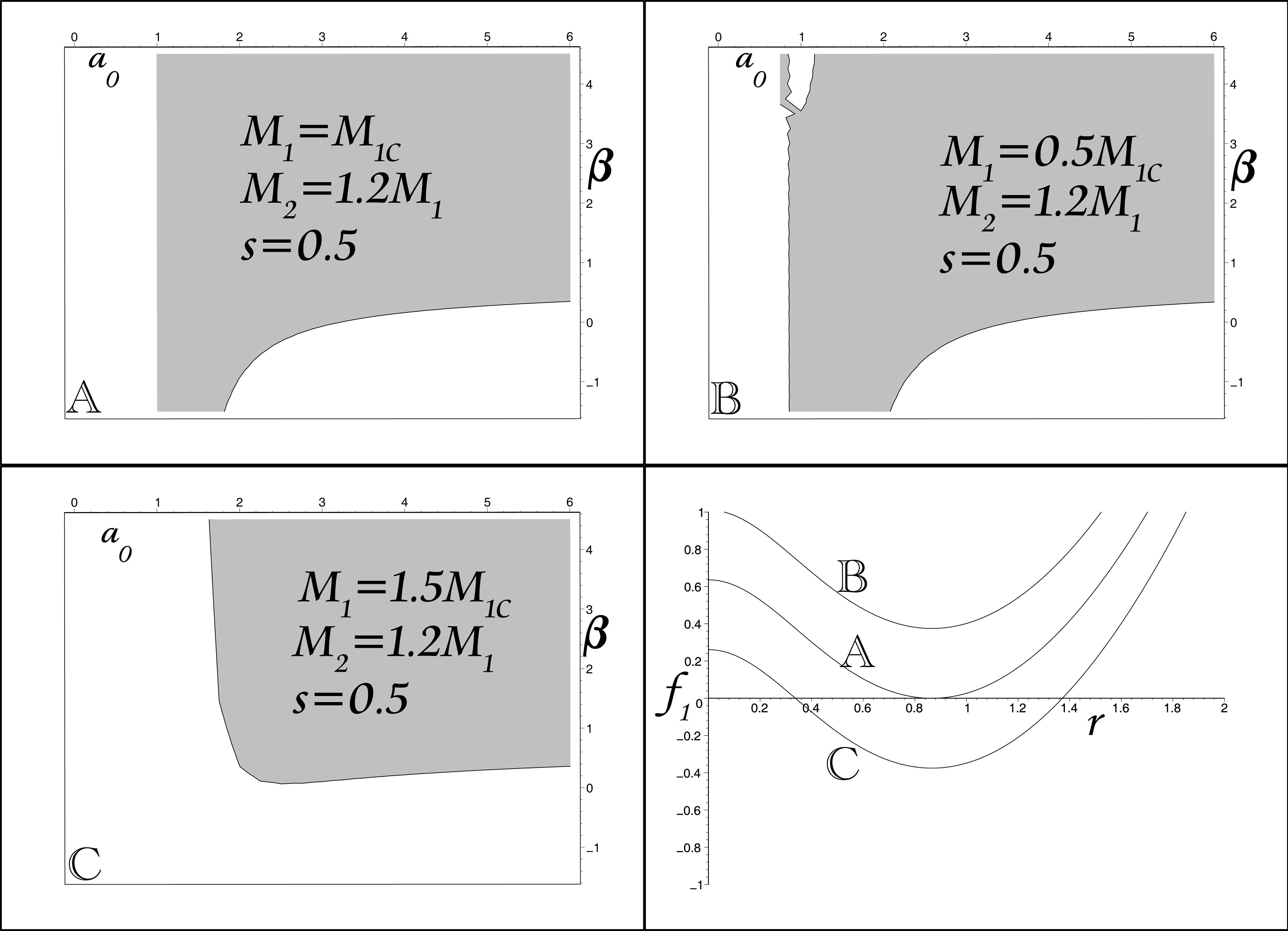
Figure 1: A plot of $V^{\prime\prime}\left(a_{0}\right)$ versus $\beta$ and $a_{0}$ with $Q=1,\ell^{2}=1$ and $M_{1}=M_{1c}$ in (A) $M_{1}=0.5M_{1c}$ in (B) and $M_{1}=1.5M_{1c}$ in (C). For all three plots $M_{2}=1.2M_{1}$ and $s=0.5.$ In the right bottom we also plot the metric function for $r<a_{0}$ to show that the possible horizon remains inside the thin shell. Figures (A) and (B) manifest stability for the thin shell against a linear perturbation.

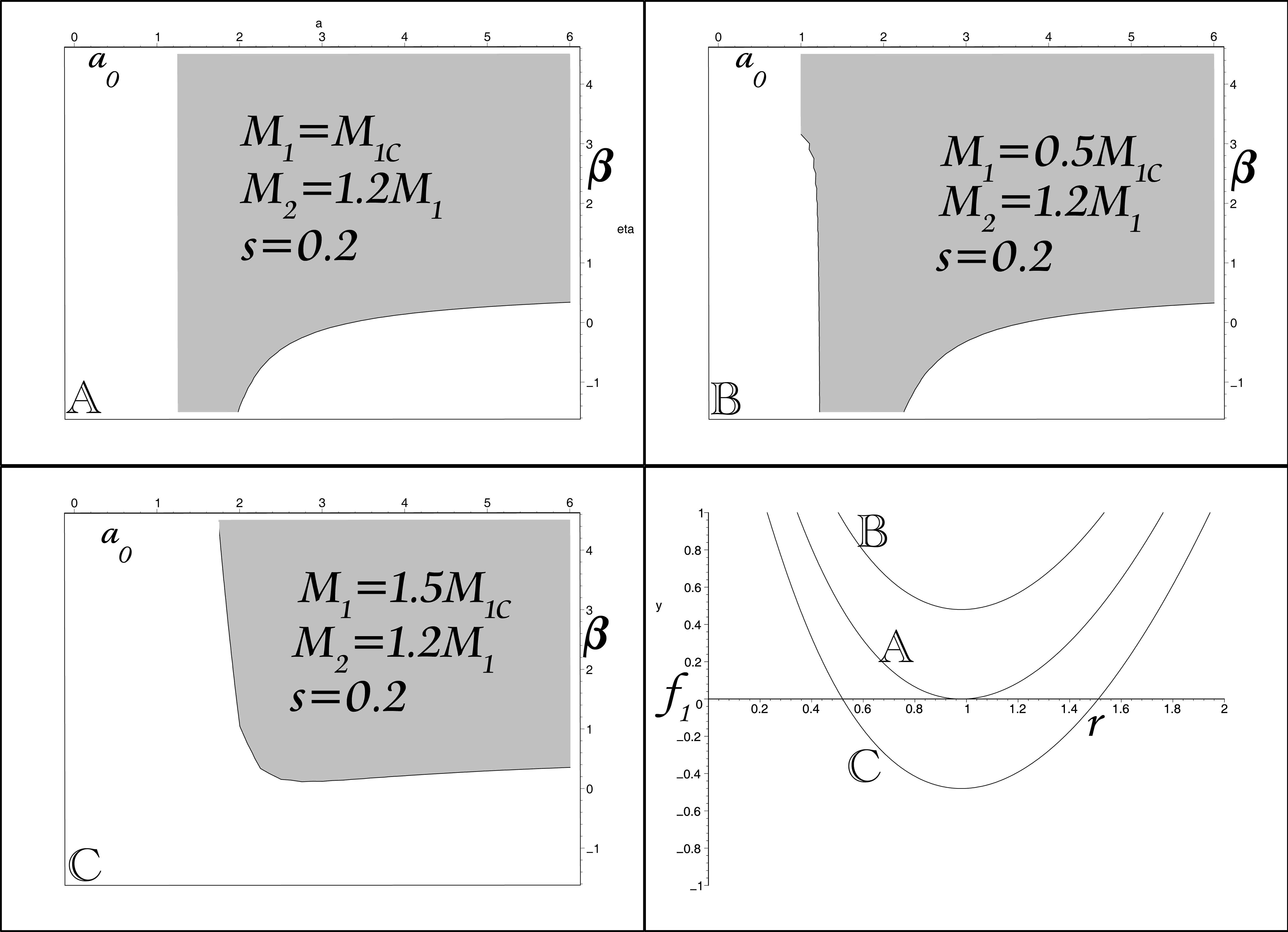
Figure 2: A plot of $V^{\prime\prime}\left(a_{0}\right)$ versus $\beta$ and $a_{0}$ with $Q=1,\ell^{2}=1$ and $M_{1}=M_{1c}$ in (A) $M_{1}=0.5M_{1c}$ in (B) and $M_{1}=1.5M_{1c}$ in (C). For all three plots $M_{2}=1.2M_{1}$ and $s=0.2.$ In the right bottom we also plot the metric function for $r<a_{0}$ to show that the possible horizon remains inside the thin shell. Figures (A) and (B) manifest stability for the thin shell against a linear perturbation.

$$\sigma=\left(\frac{a}{a_{0}}\right)^{1+\beta}\left(\sigma_{0}+\frac{p_{0}}{1+\beta}\right)-\frac{p_{0}}{1+\beta}.$$ (44)

The dynamic of the energy density also is given by (39) which together imply a one dimensional equation of motion for the shell is given by

$$\dot{a}^{2}+V\left(a\right)=0$$ (45)

with

$$V\left(a\right)=\frac{f_{1}\left(a\right)+f_{2}\left(a\right)}{2}-\left(\frac{f_{1}\left(a\right)-f_{2}\left(a\right)}{16\pi a\sigma}\right)^{2}-\left(4\pi a\sigma\right)^{2}.$$ (46)

At the equilibrium $V\left(a_{0}\right)=V^{\prime}\left(a_{0}\right)=0$ and the first nonzero term is the second derivative of the potential at $a=a_{0}$ which must be positive to have an oscillatory motion for the shell upon linear perturbation. This in turn means that the shell will be stable. In Fig.s 1 and 2 we plot the region in which $V^{\prime\prime}\left(a_{0}\right)\geq 0$ or the stable regions with

$$f_{1}\left(a\right)=-M_{1}+\frac{a^{2}}{\ell^{2}}-Q_{1}^{2}\ln\left(a^{2}+s^{2}\right)$$ (47)

and

$$f_{2}\left(a\right)=-M_{2}+\frac{a^{2}}{\ell^{2}}.$$ (48)

To do so we used a critical mass

$$M_{1c}=Q^{2}\left[1-\ln\left(Q^{2}\ell^{2}\right)\right]-\frac{s^{2}}{\ell^{2}}$$ (49)

at which for $M_{1}>M_{1c}$ a black hole with two horizons forms inside the thin-shell and for $M_{1}<M_{1c}$ the solution for inside thin-shell is non-black hole while $M_{1}=M_{1c}$ represents the extremal black hole inside the thin-shell. We note that a distant observer does not detect any electric charge of the black hole. Therefore the black hole structure of the spacetime inside the shell may not be seen even though $a$ was supposed to be larger than the horizon. In this case the thin-shell carries a charge $Q_{2}=-Q_{1}$ which completely shields the black hole nature of the spacetime. In fact Fig.s 1 and 2 show that the thin-shell is stable for all values of $\beta$ irrespective of whether we have an extremal black hole or no black hole at all. However in the case of non-black hole solution which are shown in Fig.s 1B and 2B, if the initial radius of the ring $a_{0}$ (which is also the equilibrium radius) is set less than $r_{\min}$ in which $f_{1}^{\prime}\left(r_{\min}\right)=0$, such perturbation may make the ring to collapse to a point. In such case still there is no singularity and the remained spacetime is BTZ solution. Furthermore, since the internal black hole is regular, the thin-shell behaves like an ordinary object with no singularity inside.

IV Conclusion

No doubt, Einstein / Einstein-Maxwell theory has limited scopes in $2+1-$dimensional spacetimes which has been studied extensively during the recent decade 8 . With non-linear electrodynamics (NED) fresh ideas has been pumped into the spacetime and served well as far as removal of singularities is concerned 10 ; 14 . Most of the black hole properties in $3+1-$dimensional spacetime has counterparts in $2+1-$dimensions with yet some differences. One common property is the existence of regular Bardeen black hole which is sourced by a radial electric field in $2+1-$dimensions whereas the source in $3+1-$dimensions happened to be magnetic. By encircling the central regular Bardeen black hole by a charged thin-shell and matching inside to outside in accordance with the Lanczos’ conditions we erase the entire effect of charge to the outside world. Such a thin-shell (or ring) doesn’t seem a mere illusion, but is a reality since it turns out to be stable against linear perturbations. The idea works in the case of a regular interior black hole well but remains to be proved whether it is applicable for a singular black hole. From astrophysical point of view is it possible that a natural, concentric thin-shell with equal (but opposite) charge to that of a central black hole forms to cancel external effect of charge at all? Admittedly our analysis here relates only to the $2+1-$dimensional case but it is natural to expect a similar charge screening effect in higher dimensions as well.

References

- (1) M. Cataldo and A. García, Phys. Rev. D 61, 084003 (2000).
- (2) M. Born and L. Infeld, Foundations of the New Field Theory. Proc. Roy. Soc, A 144, 425 (1934).
- (3) E. Ayón-Beato and A. Garciá, Phys. Rev. Lett. 80, 5056 (1998); E. Ayón-Beato and A. García, Phys. Lett. B 464, 25 (1999).
- (4) J. M. Bardeen, et al, Commun. Math. Phys. 31, 161 (1973); S. A. Hayward, Phys. Rev. Lett. 96, 031103 (2006); J. Bardeen, abstract in Proceedings of GR5, Tiflis, USSR (1968); I. Dymnikova, Gen. Relativ. Gravit. 24, 235 (1992); Int. J. Mod. Phys. D 5, 529 (1996); Classical Quantum Gravity 19, 725 (2002); Int. J. Mod. Phys. D 12, 1015 (2003). M. Mars, M. M. Martín-Prats, and J. M. M. Senovilla, Classical Quantum Gravity 13, L51 (1996); A. Borde, Phys. Rev. D 55, 7615 (1997); M. R. Mbonye and D. Kazanas, Phys. Rev. D 72, 024016 (2005); I. Dymnikova, Classical and Quantum Gravity, 21, 4417 (2004); K. Lin, J. Li, S. Yang and X. Zu, Int. J. Theor. Phys. 52, 1013 (2013); S. Hossenfelder, L. Modesto and I. Prémont-Schwarz, Phys. Rev. D 81, 044036 (2010); K. A. Bronnikov and J. C. Fabris, Phys. Rev. Lett. 96, 251101 (2006); K. A. Bronnikov, Phys. Rev. D 63, 044005 (2001); K. A. Bronnikov, Phys. Rev. Lett. 85, 4641 (2000); N. Uchikata, S. Yoshida and T. Futamase, Phys. Rev. D 86, 084025 (2012).
- (5) W. Israel, Nuovo Cimento B 44, 1 (1966); 48, 463(E) (1967). W. Israel, Nuovo Cimento 66, 1 (1966).
- (6) S. H. Mazharimousavi and M. Halilsoy, ”A new Einstein-nonlinear electrodynamics solution in dimensions” arXiv:1304.5206.
- (7) N. Sen, Ann. Phys. (Leipzig) 378, 365 (1924); K. Lanczos, ibid. 379, 518 (1924); G. Darmois, Me´morial des Sciences Mathematiques, Fascicule XXV (Gauthier-Villars, Paris, 1927), Chap. 5; E. F. Eiroa, and C. Simeone, Phys. Rev. D 87, 064041 (2013).
- (8) M. Bãnados, C. Teitelboim and J. Zanelli, Phys. Rev. Lett. 69, 1849 (1992); M. Banados, M. Henneaux, C. Teitelboim and J. Zanelli, Phys. Rev. D 48, 1506 (1993); C. Martınez, C. Teitelboim and J. Zanelli, Phys. Rev. D 61, 104013 (2000).
- (9) J. D. Brown and J.W. York, Phys. Rev. D 47, 1407 (1993); J. D. Brown, J. Creighton and R. B. Mann, Phys. Rev. D 50, 6394 (1994).
- (10) M. Cataldo, N. Cruz, S. del Campo and A. Garcia, Phys. Lett. B 484, 154 (2000).
- (11) Y. S. Myung, Y.-W. Kim and Y.-J. Park, Phys. Rev. D 78, 044020 (2008).
- (12) J. Crisóstomo and R. Olea, Phys. Rev. D 69, 104023 (2004); R. Olea, Mod. Phys. Lett. A 20, 2649 (2005); R. B. Mann and J. J. Oh, Phys. Rev. D 74, 124016 (2006); 77, 129902(E) (2008); R. B. Mann, J. J. Oh, and M.-I. Park, 79, 064005 (2009).
- (13) P. Musgrave and K. Lake, Classical Quantum Gravity 13, 1885 (1996); P. R. Brady, J. Louko, and E. Poisson, Phys. Rev. D 44, 1891 (1991); M. Ishak and K. Lake, Phys. Rev. D 65, 044011 (2002); S. M. C. V. Gonçalves, Phys. Rev. D 66, 084021 (2002); F. S. N. Lobo and P. Crawford, Classical Quantum Gravity 22, 4869 (2005); M. Visser, Lorentzian Wormholes (AIP Press, New York, 1996); E. Poisson and M. Visser, Phys. Rev. D 52, 7318 (1995).
- (14) L. Balart, Mod. Phys. Lett. A 24, 2777 (2009); S. H. Mazharimousavi, O. Gurtug, M. Halilsoy and O. Unver, Phys. Rev. D 84, 124021 (2011); O. Gurtug, S. H. Mazharimousavi, M. Halilsoy, Phys. Rev. D 85, 104004 (2012); S. H. Hendi, Journal of High Energy Physics 2012, 65 (2012).