Major open problems in chaos theory and nonlinear dynamics

Abstract.

Nowadays, chaos theory and nonlinear dynamics lack research focuses. Here we mention a few major open problems: 1. an effective description of chaos and turbulence, 2. rough dependence on initial data, 3. arrow of time, 4. the paradox of enrichment, 5. the paradox of pesticides, 6. the paradox of plankton.

1. Introduction

Chaos theory originated from studies in classical mechanics (H. Poincaré [24]), fluid mechanics (E. Lorenz [19]), and ecology (R. May [20]). By now chaos theory has spread to almost every scientific area and beyond. Overall, chaos is understood but not tamed. In fact, it is not clear whether or not it is tractable! More specifically, the mechanism of how chaotic dynamics operates is understood; how to effectively describe chaos in term of some sort of averaging is beyond reach (i.e. not tamed); it is not even clear what kind of averaging mean we should be after for! These questions will form the first major open problem to be discussed below. Returning to the three specific areas where chaos theory originated, chaotic dynamics in classical mechanics is understood; chaotic dynamics (turbulence) in fluid mechanics is being understood in infinite dimensional phase space under the flow defined by Navier-Stokes equations; chaotic dynamics (and nonlinear dynamics in general) in ecology is not (or poorly) understood. In classical mechanics, dynamics is generally governed by a system of finitely many ordinary differential equations, and numerical simulations of such a system have very good precision and can in principle reveal all the detailed structures in the finite dimensional phase space. In fluid mechanics, dynamics is governed by Navier-Stokes equations. The phase space is infinite dimensional. Numerical simulations on Navier-Stokes equations have a long way from accuracy. Nevertheless, explorations on nonwandering structures such as fixed points (steady states), periodic orbits, homoclinic orbits, and bifurcations to chaos have established reliable results [22] [30] [29] [9]. Philosophically speaking, chaos in fluid is a part of turbulence. The question is whether or not turbulence contains more. This question will be addressed in the second open problem below: rough dependence on initial data. The initiation (onset) of turbulence is much trickier [16] [11] than that of chaos in finite dimensions. In ecology [21], the accuracy of various mathematical models is difficult to test. Large scale field studies are difficult to conduct. These difficulties lead to the poor understanding of nonlinear dynamics in ecology.

Chaos theory forms the core of a greater area called complex systems. Even though there has been tremendous effort in the grand area of complex systems, no substantial new scientific result has been obtained. Nowadays, research in the area of chaos theory lacks focus, partly due to its spreading into the area of complex systems, and partly due to its spreading into almost all scientific areas. Here we shall mention a few major open problems which we believe to be of fundamental importance in chaos theory and nonlinear dynamics.

2. An effective description of chaos and turbulence

The search for an effective description of turbulence started from Reynolds average [25] [6]. Reynolds average was designed for a stochastic signal which is the sum of an average signal and a small stochastic perturbative signal. Unfortunately chaos and turbulence are far from such stochastic signals. Thus Reynolds average is far from an effective description of turbulence. Applying Reynolds average to chaos and turbulence will inevitably lead to an unsolvable closure problem. Since turbulence is chaos under Navier-Stokes flow, it is a good idea to first search for an effective description for chaos of simple systems. In fact, one can view fractal dimension [2] and SRB measure [1] for strange attractor as description of chaos. Fractal dimension does not have much engineering value. SRB measure is elusive for most of systems. Thus neither fractal dimension nor SRB measure is an effective description of chaos. Horseshoe [28] [13] and shadowing [23] [14] in combination with Bernoulli shift are also descriptions of chaos. Shadowing has the greatest potential to generate an effective description of chaos [15] [10]. But with the current computer capacity, shadowing of the entire turbulent attractor is still beyond reach. A description of turbulence which is effective in engineering means a solution of the problem of turbulence.

3. Rough dependence on initial data

The signature of chaos is ”sensitive dependence on initial data”, here I want to address ”rough dependence on initial data” which is very different from sensitive dependence on initial data. For solutions (of some system) that exhibit sensitive dependence on initial data, their initial small deviations usually amplify exponentially (with an exponent named Liapunov exponent), and it takes time for the deviations to accumulate to substantial amount (say order $O(1)$ relative to the small initial deviation). If $\epsilon$ is the initial small deviation, and $\sigma$ is the Liapunov exponent, then the time for the deviation to reach $1$ is about $\frac{1}{\sigma}\ln\frac{1}{\epsilon}$. On the other hand, for solutions that exhibit rough dependence on initial data, their initial small deviations can reach substantial amount instantly. Take the 3D or 2D Euler equations of fluids as the example, for any $t\neq 0$ (and small for local existence), the solution map that maps the initial condition to the solution value at time $t$ is nowhere locally uniformly continuous and nowhere differentiable [8]. In such a case, any small deviation of the initial condition can potentially reach substantial amount instantly. My conjecture is that the high Reynolds number violent turbulence is due to such rough dependence on initial data, rather than sensitive dependence on initial data of chaos. When the Reynolds number is sufficiently large ( the viscosity is sufficiently small), even though the solution map of the Navier-Stokes equations is still differentiable, but the derivative of the solution map should be extremely large everywhere since the solution map of the Navier-Stokes equations becomes the solution map of the Euler equations when the viscosity is zero (the Reynolds number is set to be infinity). Such everywhere large derivative of the solution map of the Navier-Stokes equations should manifest itself as the development of violent turbulence in a short time. In summary, not large enough Reynolds number turbulence may be due to sensitive dependence on initial data of chaos, while large enough Reynolds number turbulence may be due to rough dependence on initial data.

The type of rough dependence on initial data shared by the solution map of the Euler equations is difficult to find in finite dimensional systems. The solution map of the Euler equations is still continuous in initial data. Such a solution map (continuous, but nowhere locally uniformly continuous) does not exist in finite dimensions. This may be the reason that one usually finds chaos (sensitive dependence on initial data) rather than rough dependence on initial data. If the solution map of some special finite dimensional system is nowhere continuous, then the dependence on initial data is rough, but may be too rough to have any realistic application.

4. The arrow of time

The arrow of time generally refers to the phenomenon of microscopic time reversibility v.s. macroscopic time irreversibility. That is, macroscopically there is an arrow of time. The arrow of time is an important problem in several branches of physics. We believe that it is also an important problem in chaos theory. A simple example of the arrow of time in chaos theory is the problem of releasing bouncing balls in the half box to the whole box. Due to the chaotic dynamics of the bouncing balls, after sufficiently long time, even though every ball’s velocity is simultaneously reversed, the chance of all the balls simultaneously return to the half box is very small ($2^{-N}$ where $N$ is the number of balls) [17]. The inevitable perturbations amplify substantially via chaotic dynamics after enough time, see Figures 1 and 2. The chaotic dynamics liberates the mathematical control of the Newtonian law to the balls so that after sufficiently long time, the orbits of the balls loose the memory of the initial condition, and are far away from the purely mathematical orbits! When the number of balls increases, e.g. the case of gas molecules, the problem becomes a problem of thermodynamics. In thermodynamics, the arrow of time refers to the second law of thermodynamics in which the entropy can only change in one direction (i.e. the time’s arrow). Our diagram of the arrow of time in thermodynamics is shown in Figure 3. The term, arrow of time, was introduced by Arthur Eddington in 1927. Now several types of arrows of time have been studied. These include thermodynamic, cosmological, psychological, and causal arrows of time. Cosmological arrow of time means the universe’s expansion, psychological arrow of time means that one can only remember the past not the future, and causal arrow of time means that cause precedes its effect. The mechanisms of these different arrows of time may be different. Chaos theory seems to be most directly relevant to the thermodynamic arrow of time. For the cosmological arrow of time, one may ask the question: Is the universe still expanding if the velocity of every object (or every molecule) is simultaneously reversed? If the answer is yes, then chaos theory may still be relevant. Even though brain dynamics may be chaotic, the direct relevance of chaos theory to the psychological arrow of time is not clear. The relevance of chaos theory to the causal arrow of time is even more unclear.

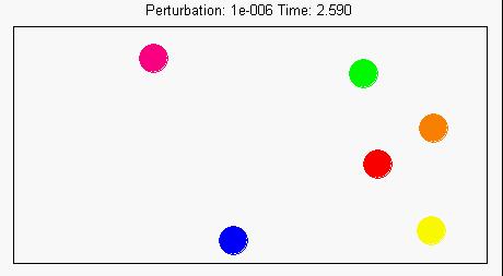
(a) $t=2.59$

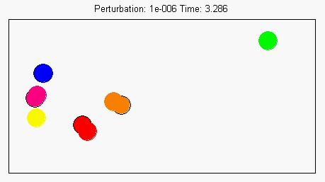
(b) $t=3.286$

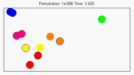
(c) $t=3.42$

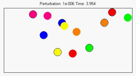
(d) $t=3.954$

Figure 1. The evolution of the six disks and the evolution of the perturbed six disks. Since the perturbation size is $10^{-6}$, initially the unperturbed and the perturbed disks coincide almost completely. The radius of the disk is $0.25$, and the rectangle domain is $8\times 4$.

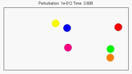
(a) $t=3.608$

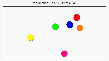
(b) $t=4.046$

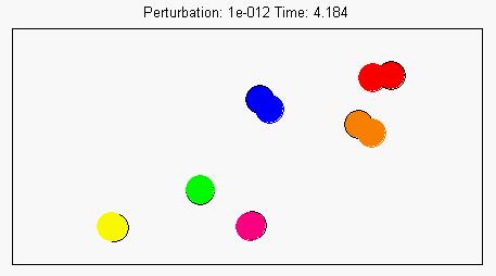
(c) $t=4.184$

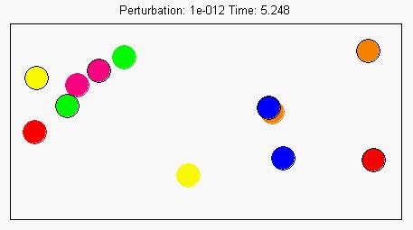
(d) $t=5.248$

Figure 2. The same setup as in Figure 1 except that the perturbation size is $10^{-12}$.

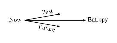
Figure 3. The diagram of the arrow of time. The ‘Past’, ‘Now’ and ‘Future’ are coordinate time, and the ‘Entropy’ is the thermodynamic equilibrium entropy.

5. The paradox of enrichment

The paradox of enrichment was first observed by M. Rosenzweig [26] in a class of mathematical models on the dynamics of predators and prey. The paradox roughly says that the class of mathematical models predicts that increasing the nutrition to the prey may lead to the extinction of both the prey and the predator. The most important question is whether or not this paradox can be observed experimentally. It is possible that the paradox is purely an artifact of the mathematical models, while in reality increasing the nutrition to the prey never leads to an extinction. If that is the case, then developing better mathematical models is necessary.

Specifically let us look at one of such mathematical models [26],

(5.1) $$\frac{dU}{dT}=\alpha U\left(1-\frac{U}{b}\right)-\gamma\frac{U}{U+h}V,$$

(5.2) $$\frac{dV}{dT}=\left(\kappa\gamma\frac{U}{U+h}-\mu\right)V,$$

where $U$ is the prey density, $V$ is the predator density, $T$ is the time coordinate, $\alpha$ is the maximal per capita birth rate of the prey, $b$ is the carrying capacity of the prey from the nutrients, $h$ is the half-saturation prey density for predation, $\gamma$ is the coefficient of the intensity of predation, $\kappa$ is the coefficient of food utilization of the predator, and $\mu$ is the mortality rate of the predator. The paradox focuses upon the steady state given by

$$\kappa\gamma\frac{U}{U+h}-\mu=0,\ \alpha\left(1-\frac{U}{b}\right)-\gamma\frac{1}{U+h}V=0.$$

It turns out that when other parameters are fixed, increasing $b$ leads to the loss of stability of this steady state, in which case, a limit cycle attractor around the steady state is generated. As $b$ increases, the limit cycle gets closer and closer to the $V$-axis. That is, along the limit cycle attractor, the prey population $U$ decreases to a very small value. Under the ecological random perturbations, $U$ can reach $0$, i.e. extinction of the prey. With the extinction of the prey, the predator will become extinct soon. On the other hand, increasing $b$ means increasing the carrying capacity of the prey, which can be implemented by increasing the prey’s nutrients, i.e. enrichment of the prey’s environment. Intuitively, increasing $b$ should enlarge the prey population and make it more robust from extinction. This is the paradox of enrichment. In order to resolve the paradox of enrichment, it is fundamental to rewrite the system (5.1)-(5.2) in the dimensionless form [3]:

(5.3) $$\frac{du}{dt}=u(1-u)-\frac{u}{u+H}v,$$

(5.4) $$\frac{dv}{dt}=k\left(\frac{u}{u+H}-r\right)v,$$

where $u=U/b$, $v=V\gamma/(\alpha b)$, $t=\alpha T$, and the dimensionless numbers are given by

(5.5) $$H=\frac{h}{b},\ r=\frac{\mu}{\kappa\gamma},\ k=\frac{\kappa\gamma}{\alpha}.$$

We name $H$: the capacity-predation number, and $r$: the mortality-food number.

• The Resolution [3]: Unlike the original form of the model (5.1)-(5.2), the dimensionless form of the model (5.3)-(5.4) is governed by $3$ dimensionless numbers $H$, $r$ and $k$ (5.5). $H$ is a ratio of the half-saturation $h$ and carrying capacity $b$, while $r$ and $k$ are independent of $h$ and $b$. Increasing the carrying capacity $b$ (for fixed half-saturation $h$) and decreasing the half-saturation $h$ (for fixed carrying capacity $b$) have the same effect on the capacity-predation number $H$, that is, $H$ decreases. Decreasing the half-saturation $h$ implies more aggressive predation (especially when the prey population $U$ is small), see Figure 4. Notice that

  $$\text{As }U\rightarrow 0^{+},\ \frac{U}{U+h}\rightarrow 1;$$

  and

  $$\frac{d}{dU}\frac{U}{U+h}\bigg{|}_{U=0}=1/h.$$

  Since there is no paradox between more aggressive predation (especially when the prey population $U$ is small) and extinction of prey, the paradox of enrichment now reduces to a paradox between more aggressive predation (decreasing the half-saturation $h$) and enrichment (increasing the carrying capacity $b$). As mentioned above, the special feature of the model (5.3)-(5.4) is that more aggressive predation (decreasing $h$) and enrichment (increasing $b$) is not a paradox, and results in the same effect on the governing dimensionless number $H$. This offers a resolution to the so-called paradox of enrichment.

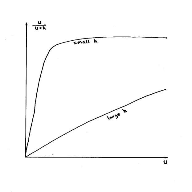
Figure 4. The predation graphs.

From the above analysis, we can see that the paradox is purely generated by the particular mathematical model. If we replace the predation term $\frac{U}{U+h}$ in both (5.1) and (5.2) by $U$ (a mild predation when $U$ is small), the paradox disappears.

6. The paradox of pesticides

Unlike the paradox of enrichment, the paradox of pesticides was observed in experiments [5] [4] [12]. The paradox of pesticides says that pesticides may dramatically increase the population of a pest when the pest has a natural predator. Right after the application of the pesticide, of course the pest population shall decrease (so shall the predator). But the pest may resurge later on in much more abundance resulting in a population well beyond the crop’s economic threshold. Roughly speaking, the pesticide reduces the populations of both the pest and its predator, and the ratio of the population of the pest to the population of the predator is changed so that the resurgent pest population can be much more in abundance. To guide the application of pesticide in such a circumstance, a good mathematical model will be important. From the perspective of mathematical models, the phenomenon can be easily understood [18]. To model the effect of pesticides on pest resurgence, a simple mathematical model is the Lotka-Volterra system with forcing,

(6.1) $$\frac{dH}{dt} = H(a-bP)-\alpha\Delta(t-T),$$

(6.2) $$\frac{dP}{dt} = P(bcH-d)-\beta\Delta(t-T),$$

where $H$ is the pest population, $P$ is the pest’s predator population, ($a$, $b$, $c$, $d$, $\alpha$, $\beta$) are positive constants, $\Delta(t)$ is an approximation of the delta function, and the $\Delta(t-T)$ terms represent the effects of pesticides. Specifically, we choose $\Delta(t-T)$ to be

$$\Delta(t-T)=1/\epsilon,\text{ when }t\in[T,T+\epsilon];\ \ =0,\text{ otherwise}.$$

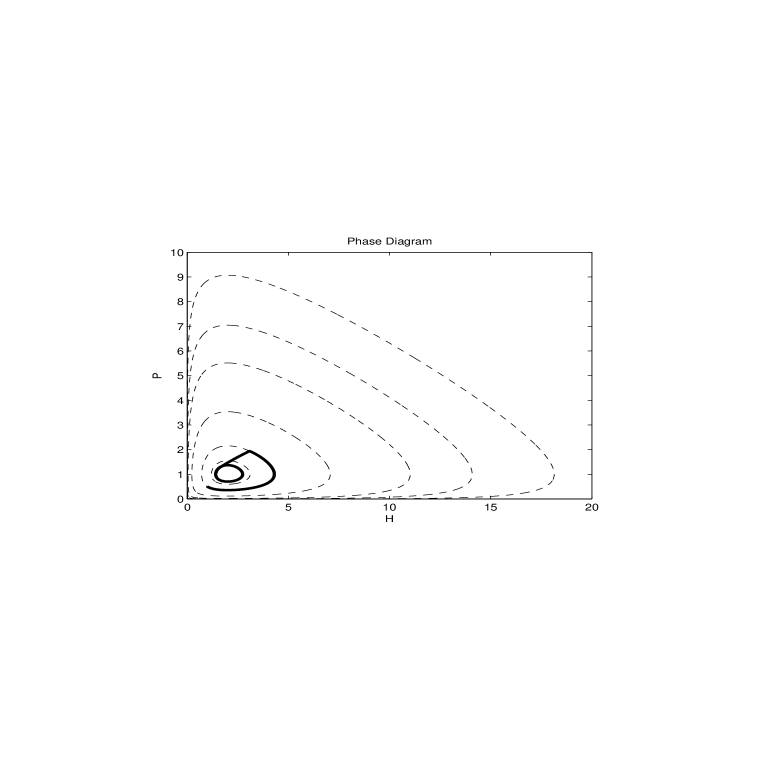
Figure 5. A pesticide forced orbit of (6.1)-(6.2), $a=b=d=1$, $c=0.5$, $T=3.5$, $\epsilon=0.07$, $\alpha=1.4$, $\beta=0.7$. In this case, the pest population deceases and maintains at a lower amplitude oscillation.

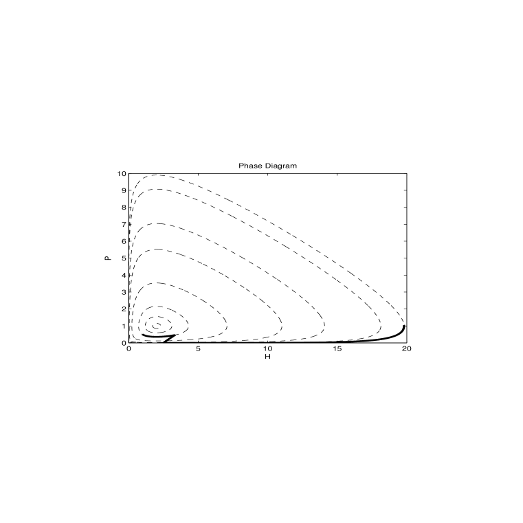
Figure 6. A pesticide forced orbit of (6.1)-(6.2), $a=b=d=1$, $c=0.5$, $T=2$, $\epsilon=0.047$, $\alpha=0.94$, $\beta=0.47$. In this case, the pest population resurges with dramatic increase beyond the crop’s economic threshold.

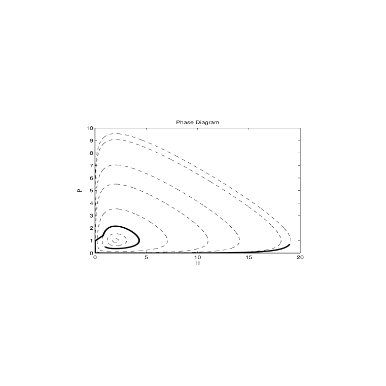
Figure 7. A pesticide forced orbit of (6.1)-(6.2), $a=b=d=1$, $c=0.5$, $T=5$, $\epsilon=0.039$, $\alpha=0.78$, $\beta=0.39$. In this case, the pest population resurges with dramatic increase beyond the crop’s economic threshold.

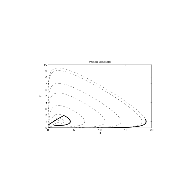
Figure 8. A pesticide forced orbit of (6.1)-(6.2), $a=b=d=1$, $c=0.5$, $T=3.5$, $\epsilon=0.149$, $\alpha=2.98$, $\beta=1.49$. In contrast to Figure 5, here large amount of pesticides is applied, and results in that the pest population resurges with dramatic increase beyond the crop’s economic threshold.

The key points on understanding the paradox of pesticides via the simple mathematical model are as follows:

1. The timing of applying the pesticides is crucial. If the pesticides are applied when the populations of both the pests and the predators are relatively large, then a decrease in both populations can be achieved, see Figure 5. On the other hand, if the pesticides are applied when either the pest’s population or the predator’s population is relatively small, then a dramatic increase in the resurgent pest’s population occurs, leading to pest’s population well beyond the crop’s economic threshold, see Figures 6 and 7. From these figures, it is clear that even though the pesticides only kill the pests rather than their predators (that is, right after the application of the pesticides, the pest’s population decreases, while the predator’s population maintains the same), the pests still resurge in abundance beyond the crop’s economic threshold. This is because that when the population of the pests decreases, the predator’s population will decreases too, since the predators feed on the pests. It is the relatively minimal values of both the pest’s population and the predator’s population that decide how large the cycle which they are going to sit on in the phase plane.

2. The amount of pesticides applied is also important. In the case of Figure 5, if the amount of pesticides is large enough, a dramatic increase in the resurgent pest’s population can still occur as shown in Figure 8.

The above conclusions also applies when spatial dependence is taken into account [18].

7. The paradox of plankton

In ecology, the Liebig’s law says that population growth is controlled not by the total amount of resources available, but by the amount of the scarcest resource (limiting factor). For instance, according to the Bateman principle, females spend more energy on generating offsprings than males do, thus females are a limiting resource over which males compete in most species. In the case of the plankton, especially phyto-plankton (in contrast to zoo-plankton), many (hundreds) species are competing for one or a few limiting resources (nutrients with severe deficiency in the summer). According to the principle of competitive exclusion, the final equilibrium state should be taken over by one or a few species according to the limiting factors. On the other hand, in reality hundreds species of the plankton coexist. This paradoxical question was first raised by Hutchinson [7]. Hutchinson proposed the idea that this is due to the fact that equilibrium state cannot be reached in reality. Since Hutchinson’s work, there have been many studies on the paradox [27]. The problem involves two branches of chaotic dynamics: fluids and ecology.

Plankton drifting in (turbulent) water is an interesting problem for chaotician to model. Let $v(t,x)$ be the three-dimensional (turbulent) water velocity, $w_{n}(t,x)$ ($n=1,2,\cdots,N$) be the plankton drifting velocities relative to water, $x\in\mathbb{R}^{3}$. In reality $v(t,x)$ is governed by the Navier-Stokes equations. Numerical simulations of the full Navier-Stokes equations are still very challenging. We can conveniently model the water velocity by a chaotic time evolution of spatial patterns (with vortex structure). We believe that the essential mechanism of the plankton drifting can be captured by such a modeling. Let $f(t,x)$ be the density of the limiting resource (deficient neutrient), and $\rho_{n}(t,x)$ be the densities of different species of plankton, $n=1,2,\cdots,N$. The model is given by

(7.1) $$\partial_{t}f+(v\cdot{\rm NewA})f=-G(\rho_{1},\rho_{2},\cdots,\rho_{N})f+F(t,x),$$

(7.2) $$\partial_{t}\rho_{n}+[(v+w_{n})\cdot{\rm NewA}]\rho_{n}=H_{n}(f)\rho_{n},\ \ n=1,2,\cdots,N,$$

where

$$G(0,0,\cdots,0)=0,$$

and $G(\rho_{1},\rho_{2},\cdots,\rho_{N})$ is strictly monotonically increasing in each $\rho_{n}$;

$$H_{n}(f^{n})=0,\ \ \text{where}\ f^{n}\ \text{are values of}\ f,$$

$H_{n}(f)$ is strictly monotonically increasing in $f$;

$$w_{n}=\kappa_{n}{\rm NewA}f+\ \text{random noise or random walk},$$

and $\kappa_{n}$ are the drifting coefficients of different plankton.

Through $G(\rho_{1},\rho_{2},\cdots,\rho_{N})$, different food consumption rates by different species of plankton can be introduced. $F(t,x)>0$ represents food regeneration, $F(t,x)$ is periodic in $t$ with relatively long period. $f^{n}$ are the ‘critical’ densities of food for different species of plankton. $H_{n}(f)$ model the growth rates from nutrition of different species of plankton.

References

- [1] K. Alligood, T. Sauer, J. Yorke, Chaos, Springer, 1997.
- [2] R. Devaney, An Introduction to Chaotic Dynamical Systems, 2nd ed., Westview Press, 2003.
- [3] Z. Feng, Y. Li, A resolution of the paradox of enrichment, submitted (2013). arXiv: 1104.4355.
- [4] H. Hamilton, The pesticide paradox, Rice Today 1 (2008), 32-33.
- [5] K. Heong, A. Manza, J. Catindig, S. Villareal, T. Jacobsen, Changes in pesticide use and arthropod biodiversity in the IRRI research farm, Outlooks on Pest Management October (2007), 1-5.
- [6] J. Hinze, Turbulence, McGraw-Hill Press, 1975.
- [7] G. Hutchinson, The paradox of the plankton, The American Naturalist XCV, No.882 (1961), 137-145.
- [8] H. Inci, On the well-posedness of the incompressible Euler equation, Dissertation, University of Zurich (2013). arXiv: 1301.5997
- [9] T. Kreilos, B. Eckhardt, Periodic orbits near onset of chaos in plane Couette flow, Chaos 22 (2012), 047505.
- [10] A. Labovsky, Y. Li, A Markov chain approximation of a segment description of chaos, Dynamics of PDE 7, no.1 (2010), 65-76.
- [11] Y. Lan, Y. Li, A resolution of the Sommerfeld paradox: numerical implementation, Intl. J. Non-Linear Mech. 51 (2013), 1-9.
- [12] P. Lester, H. Thistlewood, R. Harmsen, The effects of refuge size and number on acarine predator-prey dynamics in a pesticide-distributed apple orchard, J. Applied Ecology 35 (1998), 323-331.
- [13] Y. Li, Smale horseshoes and symbolic dynamics in perturbed nonlinear Schrödinger equations, J. Nonlinear Sci. 9 (1999), 363-415.
- [14] Y. Li, Chaos and shadowing lemma for autonomous systems of infinite dimensions, J. Dynamics Diff. Eq. 15, no.4 (2003), 699-730.
- [15] Y. Li, Segment description of turbulence, Dynamics of PDE 4, no.3 (2007), 283-291.
- [16] Y. Li, Z. Lin, A resolution of the Sommerfeld paradox, SIAM J. Math. Anal. 43, no.4 (2011), 1923-1954.
- [17] Y. Li, H. Yang, On the arrow of time, submitted (2012). arXiv: 1012.3764.
- [18] Y. Li, Y. Yang, On the paradox of pesticides, submitted (2012). arXiv: 1303.2681
- [19] E. Lorenz, Deterministic nonperiodic flow, J. Atmos. Sci. 20 (1963), 130-141.
- [20] R. May, Simple mathematical models with very complicated dynamics, Nature 261 (1976), 459-467.
- [21] R. May, Unanswered questions in ecology, Phil. Trans. R. Soc. Lond. B 354 (1999), 1951-1959.
- [22] M. Nagata, Three-dimensional finite-amplitude solutions in plane Couette flow: bifurcation from infinity, J. Fluid Mech. 217 (1990), 519-527.
- [23] K. Palmer, Exponential dichotomies, the shadowing lemma, and transversal homoclinic points, Dynamics Reported 1 (1988), 265-306.
- [24] H. Poincaré, Les Méthodes Nouvelles de la Mécanique Celeste, vol.I, II, III, 1892. English translation: New Methods of Celestial Mechanics, ed. by D. Goroff, AIP Press, 1992.
- [25] O. Reynolds, On the dynamical theory of incompressible viscous fluids and the determination of the criterion, Phil. Trans. Roy. Soc. Lond. A 186 (1895), 123-164.
- [26] M. Rosenzweig, Paradox of enrichment: destabilization of exploitation ecosystem in ecological time, Science 171 (1971), 385-387.
- [27] S. Roy, J. Chattopadhyay, Towards a resolution of ‘the paradox of the plankton’: A brief overview of the proposed mechanisms, Ecological Complexity 4 (2007), 26-33.
- [28] S. Smale, Differentiable dynamical systems, Bull. AMS 73, no.6 (1967), 747-817.
- [29] L. van Veen, G. Kawahara, Homoclinic tangle on the edge of shear turbulence, Phys. Rev. Lett. 107 (2011), 114501.
- [30] D. Viswanath, Recurrent motions with plane Couette turbulence, J. Fluid Mech. 580 (2007), 339-358.