Unification scale vs. electroweak-triplet mass in the SU(5)+${\bf 24_{F}}$ model at three loops

Abstract

It was shown recently that the original SU(5) theory of Georgi and Glashow, augmented with an adjoint fermionic multiplet $24_{F}$, can be made compatible both with neutrino masses and gauge coupling unification. In particular, the model predicts that either electroweak-triplet states are light, within the reach of the Large Hadron Collider (LHC), or proton decay will become accessible at the next generation of megaton-scale facilities. In this paper, we present the computation of the correlation function between the electroweak-triplet masses and the unification scale at the next-to-next-to-leading-order (NNLO). Such an accuracy on the theory side is necessary in order to settle the convergence of the perturbative expansion and to match the experimental precision on the determination of the electroweak gauge couplings at the Z-boson mass scale.

I Introduction

The quantum numbers of the Standard Model (SM) fermions together with the apparent convergence of the strong and electroweak couplings at energies below the Planck scale point towards a unified description of the SM interactions. One of the fundamental predictions of a Grand Unified Theory (GUT) is the existence of baryon and lepton number violating interactions which can manifest themselves at low energy via matter instability (for a review see for example Ref. Nath:2006ut ). Though the decay of the proton has not been observed so far, the lower bound on the proton lifetime, together with the low-energy values of the SM gauge couplings and the SM fermion masses and mixings provide us severe constraints on the class of viable GUT models.

On the other hand, the degree of complexity of GUTs, even in their simplest realizations, makes them hard to be tested. It is enough to say that one of the few absolute certainties about grand unification today is that the original SU(5) model of Georgi and Glashow (GG) Georgi:1974sy is ruled out. In particular, the failure of the minimal model can be attributed both to the lack of gauge coupling unification Ellis:1990wk ; Langacker:1991an ; Amaldi:1991cn and to the fact that an accidental $B-L$ global symmetry Wilczek:1979et , as in the SM, prevents neutrinos to be massive.

When looking for a minimal realistic extension of the GG model it would be economical (and hence predictive) if the solution to the issue of gauge coupling unification were related to the generation of neutrino masses. This is, essentially, the philosophy behind two recent proposals where an extra scalar representation $15_{H}$ Dorsner:2005fq ; *Dorsner:2005ii, or alternatively, a fermionic representation $24_{F}$ Bajc:2006ia ; *Bajc:2007zf is added to the field content of the model. In both cases, the extra degrees of freedom have the right quantum numbers to generate neutrino masses via the seesaw mechanism Minkowski:1977sc ; *GellMann:1980vs; *Yanagida:1979as; *Glashow:1979nm; *Mohapatra:1979ia; Magg:1980ut ; *Schechter:1980gr; *Lazarides:1980nt; *Mohapatra:1980yp; Foot:1988aq and restore unification by properly modifying the running of the gauge couplings. Though both the models share a similar degree of minimality, we shall restrict our discussion to the ${\rm SU(5)}+24_{F}$ model and postpone the ${\rm SU(5)}+15_{H}$ model for a future investigation.

Let us briefly recall the reason why gauge coupling unification fails within the minimal GG model. While $\alpha_{2}$ and $\alpha_{3}$ meet around $10^{16}$ GeV, the main issue is the early convergence of $\alpha_{2}$ and $\alpha_{1}$ at about $10^{13}$ GeV Ellis:1990wk ; Langacker:1991an ; Amaldi:1991cn , at odds with the bounds enforced by the nonobservation of the proton decay. More precisely, assuming no cancellations in the flavour structure of the gauge-induced proton decay rates FileviezPerez:2004hn ; Dorsner:2004xa , the latest experimental data from the Super-Kamiokande observatory Nishino:2012ipa imply a conservative lower bound on the unification scale $M_{G}$ of about $10^{15.5}\ \rm{GeV}$. Hence, the key ingredients for a viable unification pattern are additional particles charged under the ${\rm SU(2)}_{L}$ group that delay the meeting of $\alpha_{1}$ and $\alpha_{2}$. Such a role in the ${\rm SU(5)}+24_{F}$ model can be only played by the electroweak fermion and scalar triplets $(1,3,0)_{F,H}\in 24_{F,H}$, living in the $24$-dimensional representations of the SU(5) gauge group. They are predicted to be light Bajc:2006ia ; *Bajc:2007zf, eventually of $\mathcal{O}(\text{TeV})$, so that a large enough unification scale can be reached.
Both types of triplets, if light enough, can give interesting signature at the LHC. The fermionic component leads to same sign dilepton events which violate lepton number Bajc:2006ia ; *Bajc:2007zf (see Franceschini:2008pz ; delAguila:2008cj ; delAguila:2008hw ; Arhrib:2009mz ; ATLAS1 for some recent collider analysis). The bosonic triplet instead can easily modify the decay properties of the Higgs boson (see e.g. Chang:2012ta ), that will be measured with increasingly precision at the LHC.

The complete unification pattern including also the convergence of $\alpha_{3}$ with $\alpha_{1}$ and $\alpha_{2}$ requires heavier particles charged under the ${\rm SU(3)}_{C}$ group. In the ${\rm SU(5)}+24_{F}$ model these are the colour-octet fermions and scalars, $(8,1,0)_{F,H}\in 24_{F,H}$, that are predicted to live at intermediate mass scales of about $10^{8}$GeV Bajc:2006ia ; *Bajc:2007zf, well beyond the LHC energy range.

Remarkably, it can be established a correlation between the electroweak triplet masses and the unification scale which acts as a “precision observable”. Imposing the condition of gauge coupling unification, the electroweak triplet masses can be expressed through the Renormalization Group Equations (RGEs) of the model as a function of the GUT scale and the electroweak couplings $\alpha_{1}$ and $\alpha_{2}$ evaluated at the Z-boson mass scale $M_{Z}$. Given the high accuracy at which the latter parameters are determined experimentally, one can make very precise predictions for the dependence of the electroweak triplet masses on the GUT scale. Such a correlation function plays a significant role for testing the model. If the electroweak triplets are not found at the LHC, then, according to the ${\rm SU(5)}+24_{F}$ model, the predicted unification scale is smaller than about $10^{16}$ GeV. Thus, matter instability is expected to be observed in the next generation of proton decay experiments Abe:2011ts , otherwise the model is ruled out. For such an important task it is mandatory to have precise theoretical predictions at least comparable with the experimental accuracy. Let us also mention that the magnitude of the two-loop radiative corrections Bajc:2007zf to the determination of the triplet masses is comparable with that of the one-loop contributions and it is almost 10 times larger than the parametric uncertainty due to the dependence on the low-energy values of $\alpha_{1}$ and $\alpha_{2}$. Thus, a three-loop analysis is indispensable in order to establish whether the perturbative series converges and to match the experimental precision.

For a consistent three-loop prediction of the electroweak-triplet masses, one needs the RGEs of the gauge couplings for the ${\rm SU(5)}+24_{F}$ model and for all effective field theories (including the SM) that can be derived from it, at three-loop accuracy. In addition, threshold corrections induced at the heavy particle mass scales are necessary at the two-loop order. The RGEs for gauge theories based on semisimple gauge groups have been known at two-loop accuracy for a long time Machacek:1983tz ; Jack:1984vj , whereas for simple gauge groups even the three-loop order results are known Pickering:2001aq . The three-loop contributions to the RGEs of the SM Mihaila:2012fm ; Bednyakov:2012en ; Chetyrkin:2012rz have been computed recently. In this work we go a step further towards the computation of the three-loop corrections to the RGEs for a general semisimple gauge group.
The threshold corrections for a general gauge theory are known at the one-loop level also since long time Weinberg:1980wa ; *Hall:1980kf. However, general results for the two-loop contributions are not available in the literature. In this paper we also compute the two-loop threshold corrections for the relevant heavy states of the ${\rm SU(5)}+24_{F}$ model.

The paper is organised as follows: in the next Section we introduce the ${\rm SU(5)}+24_{F}$ model, specify the particle content and describe its main features. In Section III and Section IV we discuss the approach of multi-loop calculations within effective field theories using mass independent regularization and renormalization schemes. Furthermore, we present our results for the three-loop gauge beta functions and the two-loop matching coefficients for the effective theory consisting in the SM and electroweak triplets. The corresponding results for the effective theory including also colour-octet multiplets are given in Appendix B.2. In Section V, we describe the phenomenological implications of our calculation. Especially, we emphasize the effects of the three-loop corrections on the prediction of the electroweak-triplet masses. Finally in Section VI we present our conclusions and insights. In addition, we discuss in some detail, in Appendix A, the tree-level calculation of the mass spectrum of the ${\rm SU(5)}+24_{F}$ model and the relations that can be established between its parameters and the ones occurring in the low-energy effective theory.

II The SU(5) + ${\bf 24_{F}}$ model

Let us start by reviewing the basic features of the SU(5) model augmented with a fermionic $24_{F}$ multiplet. More technical aspects about the particle content, its mass spectrum and low-energy interactions are deferred into a self-contained Appendix (cf. Appendix A).

The scalar sector spans over two different representations, namely,

$$5_{H}=\underbrace{(3,1,-\tfrac{1}{3})_{H}}_{\mathcal{T}}\oplus\underbrace{(1,2,+\tfrac{1}{2})_{H}}_{h}\,,$$ (1)

and

$$24_{H}=\underbrace{(1,1,0)_{H}}_{S_{H}}\oplus\underbrace{(1,3,0)_{H}}_{T_{H}}\oplus\underbrace{(8,1,0)_{H}}_{O_{H}}\\ \oplus\underbrace{(3,2,-\tfrac{5}{6})_{H}}_{X_{H}}\oplus\underbrace{(\overline{3},2,+\tfrac{5}{6})_{H}}_{\overline{X}_{H}}\,,$$ (2)

where $S_{H}$, $T_{H}$ and $O_{H}$ ($\mathcal{T}$, $h$ and $X_{H}$) are real (complex) scalars. In our notation, $h$ stands for the SM Higgs doublet.
The decomposition of the vector bosons belonging to the SU(5) adjoint representation reads

$$24_{V}=\underbrace{(1,1,0)_{V}}_{S_{V}}\oplus\underbrace{(1,3,0)_{V}}_{T_{V}}\oplus\underbrace{(8,1,0)_{V}}_{O_{V}}\oplus\\ \underbrace{(3,2,-\tfrac{5}{6})_{V}}_{X_{V}}\oplus\underbrace{(\overline{3},2,+\tfrac{5}{6})_{V}}_{\overline{X}_{V}}\,,$$ (3)

where $S_{V}$, $T_{V}$ and $O_{V}$ denote the SM gauge bosons, while $X_{V}$ and $\overline{X}_{V}$ correspond to the super-heavy gauge bosons of the SU(5) broken phase, the so-called leptoquarks. They are responsible for the gauge-induced proton-decay rate and include, as a longitudinal component, the Goldstone boson $X_{H}$ of the SU(5) broken phase.
Finally, the matter content of the model is given by the Weyl fermions of the three SM families

$$\overline{5}_{F} =(\underbrace{\overline{3},1,+\tfrac{1}{3})_{F}}_{d^{c}}\oplus\underbrace{(1,2,-\tfrac{1}{2})_{F}}_{\ell}\,,$$ (4)

$$10_{F} =(\underbrace{\overline{3},1,-\tfrac{2}{3})_{F}}_{u^{c}}\oplus\underbrace{(3,2,+\tfrac{1}{6})_{F}}_{q}\oplus\underbrace{(1,1,+1)_{F}}_{e^{c}}\,,$$ (5)

and the additional fermionic multiplet

$$24_{F}=\underbrace{(1,1,0)_{F}}_{S_{F}}\oplus\underbrace{(1,3,0)_{F}}_{T_{F}}\oplus\underbrace{(8,1,0)_{F}}_{O_{F}}\oplus\\ \underbrace{(3,2,-\tfrac{5}{6})_{F}}_{X_{F}}\oplus\underbrace{(\overline{3},2,+\tfrac{5}{6})_{F}}_{\overline{X}_{F}}\,,$$ (6)

where $S_{F}$, $T_{F}$, $O_{F}$ ($X_{F}$) are Majorana (Dirac) degrees of freedom. A special role in the model is played by the electroweak singlet and triplet states $S_{F}$ and $T_{F}$. They are involved in the Yukawa interactions that after the SU(5) gauge-symmetry breaking will generate masses for neutrinos through a hybrid type-I+III seesaw mechanism Bajc:2006ia ; *Bajc:2007zf (for details see Appendix A.2.2). The electroweak singlet $S_{F}$ resembles a sterile neutrino, whereas the electroweak triplet is sometimes referred to as a heavy lepton.

Let us mention at this point that, as in the original SU(5) model, nonrenormalizable operators are required in order to reproduce fermion masses and mixing Ellis:1979fg ; Dorsner:2006hw . Furthermore, the Higgs sector is the one of the genuine SU(5) model and the minimization of the scalar potential proceeds as usual (for details of the calculation see Appendix A.2.1). All the states are subject to the constraints coming from the calculation of the tree-level spectrum. In this respect, though the required mass hierarchy strengthen the fine-tuning issue typical for GUTs, it is nevertheless a nontrivial fact that the tree-level calculation of the spectrum allows the mass pattern required by unification Bajc:2006ia ; *Bajc:2007zf (for more details see also Appendix A.2).

III Effective field theory approach

In the following, we concentrate on the study of the gauge coupling unification assuming the mass hierarchy

$$m_{T_{F}}\approx m_{T_{H}}\ll m_{O_{F}}\approx m_{O_{H}}\ll M_{G}\,.$$ (7)

For such a largely split mass spectrum, it is convenient to apply the method of effective field theories (EFTs). This approach was introduced a long time ago in the context of GUTs Weinberg:1980wa ; Hall:1980kf and has been extensively applied in the context of the SM and its supersymmetric extension even in high precision calculations (see for example Refs. Schroder:2005hy ; Chetyrkin:2005ia ; Kurz:2012ff ). It consists in integrating out the heavy degrees of freedom that cannot influence the physics at the low-energy scale.
In physical renormalizations schemes like the momentum subtraction scheme or the on-shell scheme, the effects due to heavy particle thresholds are included in the renormalization constants of the parameters. However, for the analysis of the gauge coupling unification that requires the running of the couplings over many orders of magnitude, higher order radiative corrections to the RGEs are essential. Nevertheless, their calculation beyond one-loop order in mass dependent renormalization schemes is quite involved. A much more suited scheme for this purpose is the minimal subtraction scheme ($\overline{\mbox{MS}}$) Bardeen:1978yd , for which the gauge coupling beta functions are mass independent and their computation is substantially simplified. Nevertheless, in this scheme the Appelquist-Carazzone Appelquist:1974tg theorem does not hold anymore and the threshold effects have to be taken into account explicitly. The latter are parametrized through the decoupling (or matching) coefficients. They can be computed perturbatively using the physical constraint that the Green’s functions involving light particles have to be equal in the original and the effective theory.
For the computation presented in this paper, we adopt this second method and apply it up to the third order in perturbation theory.

Because in the underlying theory we can identify three well-separated mass scales corresponding to electroweak triplets ($T_{H,F}$), colour octets ($O_{H,F}$) and GUT particles ($\mathcal{T}$, $X_{F}$ and $X_{V}$), it is natural to construct a series of three effective theories to take into account the individual mass thresholds. A summary of the individual ingredients of the calculation is given in Table 1. For the present analysis we computed the following missing pieces: (i) The three-loop RGEs for the gauge couplings of the effective theory obtained by integrating out the super-heavy (GUT) particles. We denote this EFT as SM+T+O; (ii) The three-loop RGEs for the gauge couplings of the EFT obtained by integrating out the GUT particles and the octet multiplets, that we call SM+T. In principle, a fourth effective theory can be obtained if the mass pattern of the super-heavy particles is taken into account. Especially, the mass of the $X_{F}$ state from the $24_{F}$ multiplet can be at most of the order of $M_{G}^{2}/\Lambda$ (cf. Eq. (73)). Here, $\Lambda$ is the cutoff of the effective SU(5) theory which should be chosen so that the correct $m_{b}/m_{\tau}$ ratio is reproduced and the perturbativity domain is maximized. For the purpose of comparison with Ref. Bajc:2006ia we take the value $\Lambda=100\,M_{G}$, though also lower values of $\Lambda$ are in principle viable Dorsner:2006fx . In particular, for the contribution of $X_{F}$ to the running within the SM+T+O+${\rm X_{F}}$ EFT, we employ only a two-loop analysis Machacek:1983tz , since it has a subdominant effect. Furthermore, we compute the contributions of the electroweak triplets and colour octets (both bosonic and fermionic components) to the two-loop matching coefficients of the the SM gauge couplings, while the GUT-scale thresholds are considered only at the one-loop level Weinberg:1980wa ; Hall:1980kf .

Running	$\rm{SM}$	$\rm{SM+T}$	$\rm{SM+T+O}$	$\rm{SM+T+O+X_{F}}$
Scale	$M_{Z}\to\mu_{T}$	$\mu_{T}\to\mu_{O}$	$\mu_{O}\rightarrow\mu_{X_{F}}$	$\mu_{X_{F}}\rightarrow M_{G}$
$\#$ of loops	3	3	3	2(3)
Matching	$\alpha_{i}^{\rm{SM}}\to\alpha_{i}^{\rm{SM+T}}$	$\alpha_{i}^{\rm{SM+T}}\to\alpha_{i}^{\rm{SM+T+O}}$	$\alpha_{i}^{\rm{SM+T+O}}\to\alpha_{i}^{\rm{SM+T+O+X_{F}}}$	$\alpha_{i}^{\rm{SM+T+O+X_{F}}}\to\alpha_{G}$
Scale	$\mu_{T}$	$\mu_{O}$	$\mu_{X_{F}}$	$M_{G}$
$\#$ of loops	2	2	1(2)	1(2)

Table 1: Loop corrections available for the individual steps of the running and matching procedure in the ${\rm SU(5)}+24_{F}$ model. The numbers in bold face are due to the computation performed in this work, while the numbers in parentheses indicate the last missing ingredient for a complete three-loop analysis.

IV Running and decoupling

For exemplification, we describe in the following the calculation done in the effective theory obtained integrating out the GUT particles and the colour-octet multiplets. Thus the particle content of the effective theory consists in the SM particles and the electroweak triplets.
Let us introduce at this point the framework of the calculation. The most general Lagrangian containing the renormalizable interactions of the SM fields and the ${\rm SU(2)}_{L}$ triplets $T_{H,F}$ is given by

$$\mathcal{L} =\mathcal{L}^{\rm{SM}}+\tfrac{1}{2}\left|D_{\mu}T_{H}\right|^{2}+\tfrac{1}{2}\overline{T}_{F}\,i\,\gamma^{\mu}D_{\mu}T_{F}-V^{\rm{ren}}(h,T_{H})$$

$$+\text{gauge fixing}+\text{ghosts}\,,$$ (8)

where the covariant derivative is defined as

$$D_{\mu}=\partial_{\mu}-ig_{2}\,T_{\rm{adj}}^{A}W^{A}_{\mu}\,,$$ (9)

with $T_{\rm{adj}}^{A}$ the generators of the ${\rm SU(2)}_{L}$ gauge group in the adjoint representation. They are related to the structure constants by the relation $(T_{\rm{adj}}^{A})_{BC}\equiv-if^{ABC}$. The scalar potential describing the quartic interactions $V_{\rm{4sc}}^{\rm{ren}}$, including the SM Higgs doublet $h$, reads

$$V_{\rm{4sc}}^{\rm{ren}}(h,T_{H})=\lambda_{h}\left|h\right|^{4}+\tfrac{\lambda_{T}}{2}\left|T_{H}\right|^{2}+\lambda_{hT}\,\left|h\right|^{2}\left|T_{H}\right|^{2}\,,$$ (10)

where $\lambda_{h}$ is the SM quartic coupling and $\lambda_{T}$ and $\lambda_{hT}$ are new couplings. The tree-level relations between these low-energy couplings and the Lagrangian parameters of the ${\rm SU(5)}+24_{F}$ model are given in Eqs. (86), (93) and (94) of Appendix A.3.

For later convenience we introduce the relevant coupling constants in terms of which the analytical results are presented: $\alpha_{i}=g_{i}^{2}/(4\pi)$ with $i=1,2,3$, are the gauge coupling constants $\alpha_{t}=y_{t}^{2}/(4\pi)$ where $y_{t}$ is the top-Yukawa coupling, and $\alpha_{\lambda_{h}}=\lambda_{h}/(4\pi)$, $\alpha_{\lambda_{T}}=\lambda_{T}/(4\pi)$ and $\alpha_{\lambda_{hT}}=\lambda_{hT}/(4\pi)$ denote the quartic coupling constants in the scalar sector. In the calculation, we adopt the SU(5)-like normalization of the $\alpha_{1}$ coupling. The three gauge coupling constants are related to the quantities usually used in the SM by the all-order relations

$$\alpha_{1} = \frac{5}{3}\frac{\alpha_{\rm QED}}{\cos^{2}\theta_{W}}\,,$$

$$\alpha_{2} = \frac{\alpha_{\rm QED}}{\sin^{2}\theta_{W}}\,,$$

$$\alpha_{3} = \alpha_{s}\,,$$ (11)

where $\alpha_{\rm QED}$ is the fine structure constant, $\theta_{W}$ stands for the weak mixing angle and $\alpha_{s}$ is the strong coupling constant. Let us stress that the gauge couplings that we need are those defined in the theory described by the Lagrangian given in Eq. (IV). They can be related to the SM parameters through the decoupling coefficients that we present in the next section.

Furthermore, all the group theoretical factors we encountered in the three-loop order calculation can be expressed in terms of quadratic Casimir invariants of the relevant representations of the gauge group. For a field transforming under the representation $R$ of the gauge group $G$, where the generators $R^{A}$ satisfy

$$\left[R^{A},R^{B}\right]=if^{ABC}R^{C}\,,$$ (12)

the Casimir invariants are defined as follows

$$\begin{gathered}\mbox{Tr}\,(R^{A}R^{B})=\delta^{AB}T_{R}\,,\qquad R^{A}_{ac}R^{A}_{cb}=\delta_{ab}C_{R}\,,\\ f^{ACD}f^{BCD}=\delta^{AB}C_{G}\,,\qquad\delta^{AA}=N_{G}\,.\end{gathered}$$ (13)

Here, $N_{G}$ denotes the dimension of the group. Then the following relation, $C_{R}N_{R}=T_{R}N_{G}$, where $N_{R}=\delta_{aa}$ is the dimension of representation $R$, holds as well.

In our case, the underlying gauge group is the same as the one of the SM, namely ${\rm SU(3)}_{C}\otimes{\rm SU(2)}_{L}\otimes{\rm U(1)}_{Y}$. To avoid confusion, we introduce an additional index for the Casimir invariants associated with the individual simple groups. Namely, an index $C$ for the ${\rm SU(3)}_{C}$ group, an index $L$ for the ${\rm SU(2)}_{L}$ group and finally an index $Y$ for the ${\rm U(1)}_{Y}$ group. The explicit notation and the numerical values can be found in Table 2. The numerical values for the hypercharges of the SM fermions and scalars in the SU(5) normalization can be read from the discussion after Eq. (20) and Eq. (• ‣ B.1).

${\rm SU(3)}_{C}$	${\rm SU(2)}_{L}$	${\rm U(1)}_{Y}$
$C_{G_{c}}=3$	$C_{G_{L}}=2$	$C_{G_{Y}}=0$
$C_{R_{C}}=\tfrac{4}{3}$	$C_{R_{L}}=\tfrac{3}{4}$	$Y_{R_{y}}^{2}$
$T_{R_{C}}=\tfrac{1}{2}$	$T_{R_{L}}=\tfrac{1}{2}$	$Y_{R_{y}}^{2}$
$N_{R_{C}}=3$	$N_{R_{L}}=2$	$N_{R_{Y}}=1$
$N_{G_{C}}=8$	$N_{G_{L}}=3$	$N_{G_{Y}}=1$

Table 2: Notations and numerical values for the Casimir invariants of the simple subgroups of ${\rm SU(3)}_{C}\otimes{\rm SU(2)}_{L}\otimes{\rm U(1)}_{Y}$ that occur in the three-loop calculation. Here $R$ stands for the fundamental representations.

IV.1 Beta functions

The energy dependence of the gauge couplings is controlled by the beta functions. These are defined as

$$\mu^{2}\frac{d}{d\mu^{2}}\frac{\alpha_{i}}{\pi}=\beta_{i}(\{\alpha_{j}\},\epsilon)=-\epsilon\frac{\alpha_{i}}{\pi}$$ (14)

$$-\left(\frac{\alpha_{i}}{\pi}\right)^{2}\left[a_{i}+\sum_{j}\frac{\alpha_{j}}{\pi}b_{ij}+\sum_{j,k}\frac{\alpha_{j}}{\pi}\frac{\alpha_{k}}{\pi}c_{ijk}+\ldots\right]\,,$$

with $i=1,2$ or $3$. The expression after the second equality sign gives the perturbative expansion. Here, $\epsilon=(4-d)/2$ is the regulator of Dimensional Regularization with $d$ being the space-time dimension used for the evaluation of the momentum integrals. In practice, the functions $\beta_{i}$ are obtained from the renormalization constants of the corresponding couplings that are defined as $\alpha_{i}^{\rm bare}=\mu^{2\epsilon}Z_{\alpha_{i}}\alpha_{i}$. Exploiting the fact that the bare couplings are $\mu$-independent and taking into account that $Z_{\alpha_{i}}$ may depend on all the other couplings leads to the following formula:

$$\beta_{i}=-\left[\epsilon\frac{\alpha_{i}}{\pi}+\frac{\alpha_{i}}{Z_{\alpha_{i}}}\sum_{{j},{j\neq i}}\frac{\partial Z_{\alpha_{i}}}{\partial\alpha_{j}}\beta_{j}\right]\left(1+\frac{\alpha_{i}}{Z_{\alpha_{i}}}\frac{\partial Z_{\alpha_{i}}}{\partial\alpha_{i}}\right)^{-1}\,,$$ (15)

From Eq. (15) it is clear that the renormalization constants $Z_{\alpha_{i}}\,(i=1,2,3)$ have to be computed up to three-loop order. In principle each vertex containing the gauge coupling $\alpha_{i}$ at tree level can be used in order to obtain $Z_{\alpha_{i}}$ via the Slavnov-Taylor identity

$$Z_{\alpha_{i}} = \frac{(Z_{\text{vrtx}})^{2}}{\prod_{k}Z_{k,{\text{wf}}}}\,,$$ (16)

where $Z_{\text{vrtx}}$ stands for the renormalization constant of the vertex and $Z_{k,{\text{wf}}}$ for the wave function renormalization constant; $k$ runs over all external particles.

We have computed $Z_{\alpha_{2}}$ and $Z_{\alpha_{3}}$ using the (Fadeev-Popov) ghost-gluon and the (Fadeev-Popov) ghost-$W$ vertices as they are the most economical ones with respect to (wrt) number of diagrams. For $Z_{\alpha_{1}}$, a Ward identity guarantees that there is a cancellation between the vertex and some of the wave function renormalization constants yielding

$$Z_{\alpha_{1}} = \frac{1}{Z_{Y}},$$ (17)

where $Z_{Y}$ is the wave function renormalization constant for the gauge boson of the ${\rm U(1)}_{Y}$ subgroup of the SM in the unbroken phase.

In Fig. 1 we show three-loop sample diagrams contributing to the considered two- and three-point functions. For the explicit calculation of the required renormalization constants, we use $\overline{\mbox{MS}}$ scheme accompanied by multiplicative renormalization. As it has been shown in Ref. Chetyrkin:1984xa the computation of the renormalization constants in the $\overline{\mbox{MS}}$ scheme can be reduced to the evaluation of only massless propagator diagrams. The method was successfully applied to the three-loop calculations of anomalous dimensions within $\overline{\mbox{MS}}$ or $\overline{\mbox{DR}}$ schemes Larin:1993tp ; Larin:1993tq ; Pickering:2001aq ; Harlander:2006rj ; Harlander:2009mn ; Chetyrkin:2012rz ; Mihaila:2012fm . For the present calculation, we use a well-tested chain of programs: the Feynman rules of the model are obtained with the help of the program FeynRules Christensen:2008py and translated into QGRAF Nogueira:1991ex syntax. QGRAF generates further all contributing Feynman diagrams. The output is passed via q2e Harlander:1997zb ; Seidensticker:1999bb , which transforms Feynman diagrams into Feynman amplitudes, to exp Harlander:1997zb ; Seidensticker:1999bb that generates FORM Vermaseren:2000nd code. The latter is processed by MINCER Larin:1991fz that computes analytically massless propagator diagrams up to three loops and outputs the $\epsilon$ expansion of the result.

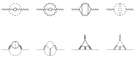
Figure 1: Sample of three-loop diagrams that appear in the calculation of $\beta$ functions. Curly lines denote gauge bosons, dotted lines ghosts, dashed lines scalar fields and solid lines fermions.

The three-loop expressions for the beta functions of the gauge couplings in the low-energy theory consisting in the SM and the electroweak triplets are given through the following formulas:

$$\beta_{1}^{\rm SM+T} =\beta_{1}^{\rm SM}$$

$$+\frac{\alpha_{1}^{2}}{\pi^{2}}\left\{\frac{\alpha_{2}^{2}}{\pi^{2}}C_{G_{L}}C_{R_{L}}N_{R_{L}}\left[\left(-\frac{11}{576}Y_{f}^{2}N_{f}-\frac{25}{576}Y_{h}^{2}N_{h}\right){N_{T_{F}}}+\left(-\frac{23}{2304}Y_{f}^{2}N_{f}-\frac{49}{2304}Y_{h}^{2}N_{h}\right){N_{T_{H}}}\right]\right.$$

$$\left.-\frac{\alpha_{\lambda_{hT}}^{2}}{\pi^{2}}\frac{1}{192}Y_{h}^{2}N_{R_{L}}N_{h}N_{G_{L}}{N_{T_{H}}}-\frac{\alpha_{\lambda_{hT}}}{\pi}\frac{\alpha_{\lambda_{h}}}{\pi}\frac{1}{8}Y_{h}^{2}N_{h}^{3}+\frac{\alpha_{2}}{\pi}\frac{\alpha_{\lambda_{hT}}}{\pi}\frac{1}{24}C_{R_{L}}Y_{h}^{2}N_{h}^{2}+\frac{\alpha_{1}}{\pi}\frac{\alpha_{\lambda_{hT}}}{\pi}\frac{1}{8}Y_{h}^{4}N_{h}^{2}\right\}\,,$$ (18)

$$\beta_{2}^{\rm SM+T} =\beta_{2}^{\rm SM}+\frac{\alpha_{2}^{2}}{\pi^{2}}\left\{C_{G_{L}}\left(\frac{1}{6}{N_{T_{F}}}+\frac{1}{24}{N_{T_{H}}}\right)+\frac{\alpha_{2}}{\pi}C_{G_{L}}^{2}\left(\frac{1}{3}{N_{T_{F}}}+\frac{7}{48}{N_{T_{H}}}\right)\right.$$

$$+\frac{\alpha_{2}^{2}}{\pi^{2}}\left[\left(\frac{247}{432}C_{G_{L}}^{3}-\frac{7}{108}C_{G_{L}}^{2}T_{R_{L}}N_{f}-\frac{11}{576}C_{G_{L}}C_{R_{L}}T_{R_{L}}N_{f}\right.\right.$$

$$\left.-\frac{127}{3456}C_{G_{L}}^{2}T_{R_{L}}N_{h}-\frac{25}{576}C_{G_{L}}C_{R_{L}}T_{R_{L}}N_{h}-\frac{145}{3456}C_{G_{L}}^{3}{N_{T_{F}}}-\frac{277}{6912}C_{G_{L}}^{3}{N_{T_{H}}}\right){N_{T_{F}}}$$

$$+\left(\frac{2749}{6912}C_{G_{L}}^{3}-\frac{13}{432}C_{G_{L}}^{2}T_{R_{L}}N_{f}-\frac{23}{2304}C_{G_{L}}C_{R_{L}}T_{R_{L}}N_{f}\right.$$

$$\left.\left.\left.-\frac{143}{6912}C_{G_{L}}^{2}T_{R_{L}}N_{h}-\frac{49}{2304}C_{G_{L}}C_{R_{L}}T_{R_{L}}N_{h}-\frac{145}{13824}C_{G_{L}}^{3}{N_{T_{H}}}\right){N_{T_{H}}}\right]\right.$$

$$+\frac{\alpha_{2}}{\pi}\frac{\alpha_{\lambda_{T}}}{\pi}\frac{5}{64}C_{G_{L}}^{2}{N_{T_{H}}^{2}}+\frac{\alpha_{2}}{\pi}\frac{\alpha_{\lambda_{hT}}}{\pi}\left(\frac{1}{24}C_{G_{L}}T_{R_{L}}N_{h}N_{T_{H}}+\frac{1}{32}T_{R_{L}}^{2}N_{h}^{2}\right)-\frac{\alpha^{2}_{\lambda_{T}}}{\pi^{2}}\frac{1}{32}C_{G_{L}}(N_{G_{L}}+2){N_{T_{H}}^{3}}$$

$$\left.+\frac{\alpha^{2}_{\lambda_{hT}}}{\pi^{2}}\left(-\frac{1}{96}C_{G_{L}}-\frac{1}{96}C_{R_{L}}\right)N_{h}{N_{T_{H}}}+\frac{\alpha_{1}}{\pi}\frac{\alpha_{\lambda_{hT}}}{\pi}\frac{1}{48}Y_{h}^{2}T_{R_{L}}N_{h}^{2}-\frac{\alpha_{\lambda_{h}}}{\pi}\frac{\alpha_{\lambda_{hT}}}{\pi}\frac{1}{16}T_{R_{L}}N_{h}^{3}\right\}\,,$$ (19)

$$\beta_{3}^{\rm SM+T}=\beta_{3}^{\rm SM}+\frac{\alpha_{3}^{2}}{\pi^{2}}\frac{\alpha_{2}^{2}}{\pi^{2}}C_{G_{L}}C_{R_{L}}N_{R_{L}}T_{R_{C}}N_{q}\\ \times\left(-\frac{11}{576}{N_{T_{F}}}-\frac{23}{2304}{N_{T_{H}}}\right)\,.$$ (20)

In the above equations $\beta_{i}^{\rm SM}$ denote the beta functions of the gauge couplings in the SM that can be found in Refs. Mihaila:2012fm ; Mihaila:2012pz . Furthermore, we use the following abbreviations: $Y_{f}^{2}N_{f}=N_{R_{C}}Y_{q}^{2}N_{q}+Y_{\ell}^{2}N_{\ell}$ and $N_{f}=N_{R_{C}}N_{q}+N_{\ell}$. The numerical values of the beta functions specified to our case are obtained by means of the following replacements: (i) $Y_{q}=\sqrt{\tfrac{3}{5}}\tfrac{1}{6}$, $Y_{\ell}=-\sqrt{\tfrac{3}{5}}\tfrac{1}{2}$, $Y_{h}=\sqrt{\tfrac{3}{5}}\tfrac{1}{2}$ denoting the hypercharges of the SM quarks, leptons and Higgs in the SU(5) normalization; (ii) $N_{q}=N_{\ell}=3$, $N_{h}=1$ and $N_{T_{F,H}}=1$ standing for the number of SM quark and lepton generations, Higgs and electroweak triplets. To recover the expressions for the beta functions in the notation of Refs. Mihaila:2012fm ; Mihaila:2012pz , we have to make the replacement $N_{q}=N_{\ell}=n_{g}$.

In order to cross-check our results, we reproduced with our setup the results for the three-loop gauge beta functions of the SM. Let us mention that we use a different implementation than the one of Refs. Mihaila:2012fm ; Mihaila:2012pz based on complete multiplets wrt the SM gauge group, e.g. left-handed leptons populating the ${\rm SU(2)}_{L}$ doublet $\ell$ are treated as the same particle in the loops, thus exploiting the full ${\rm SU(2)}_{L}$ symmetry of the unbroken SM phase. When available, we also compared the contributions generated by the electroweak triplets in the gauge sector with the results of Ref. Pickering:2001aq and obtained complete agreement.

Furthermore, the contributions of the colour octets to the beta functions in the SM+T+O model can be read from Eqs. (IV.1)–(20) after the proper substitutions. We give the results explicitly in Appendix B.1.

IV.2 Decoupling coefficients

In this section we describe the calculation of the two-loop decoupling coefficients for the SM gauge couplings when the electroweak triplets $T_{H,F}$ are integrated out. We present our results again in terms of group-theory invariants, so that our calculation can be generalized to other gauge groups as well.

Let us define at this point the decoupling coefficients for the gauge couplings when the SM+T model is matched with the SM,

$$\alpha^{\prime}_{i}(\mu)=\zeta_{\alpha_{i}}\left(\mu,\alpha_{i}(\mu),m_{T_{F,H}}(\mu)\right)\alpha_{i}(\mu)\,.$$ (21)

Here $\mu$ denotes the scale at which the decoupling of the electroweak triplets is performed. It is not fixed by the theory, but it is usually chosen of the order of the electroweak-triplet masses. It is expected that the dependence of the physical observables on this unphysical parameter is reduced order by order in perturbation theory. Such an example is illustrated in Fig. 3, in the next section. The parameters on the right-hand side of the equality are all defined in the SM+T model, whereas the SM parameters are labeled with a prime.

For the computation of the coefficient $\zeta_{\alpha_{i}}$ one has to consider Green’s functions involving light particles and a vertex that contains the gauge coupling $\alpha_{i}$. Since the matching coefficients are universal quantities, they must be independent of the momentum transfer of the specific process taken under consideration. Ref. Chetyrkin:1997un showed that the matching coefficients for the gauge couplings can be calculated from the gauge bosons and Fadeev-Popov ghost propagators and from the gauge boson-ghost vertex, all evaluated at vanishing external momenta. Thus, in dimensional regularization only diagrams containing at least one heavy particle inside the loops contribute and only the hard regions in the asymptotic expansion of the diagrams have to be taken into account. We show in Fig. 2 sample two-loop Feynman diagrams contributing to the matching coefficient for the gauge coupling $\alpha_{2}$. The Feynman diagrams are computed within our setup with the same chain of automated programs as for the calculation of the beta functions, except for the fact that the resulting Feynman amplitudes are mapped to two-loop massive tadpole topologies that are handled with the help of the program MATAD Steinhauser:2000ry .

When the electroweak triplets are integrated out, only the gauge coupling $\alpha_{2}$ is modified. Its decoupling coefficient up to two loops reads

$$\zeta_{\alpha_{2}} =1+\frac{\alpha_{2}}{\pi}C_{G_{L}}\left(-\frac{1}{6}\ln{\frac{\mu^{2}}{m_{T_{F}}^{2}}}{N_{T_{F}}}-\frac{1}{24}\ln{\frac{\mu^{2}}{m_{T_{H}}^{2}}}{N_{T_{H}}}\right)$$

$$+\left(\frac{\alpha_{2}}{\pi}\right)^{2}C_{G_{L}}^{2}\left[\left(-\frac{7}{288}-\frac{1}{12}\ln{\frac{\mu^{2}}{m_{T_{F}}^{2}}}+\frac{1}{36}\ln^{2}{\frac{\mu^{2}}{m_{T_{F}}^{2}}}{N_{T_{F}}}+\frac{1}{72}\ln{\frac{\mu^{2}}{m_{T_{F}}^{2}}}\ln{\frac{\mu^{2}}{m_{T_{H}}^{2}}}{N_{T_{H}}}\right){N_{T_{F}}}\right.$$

$$\left.+\left(\frac{37}{576}-\frac{11}{96}\ln{\frac{\mu^{2}}{m_{T_{H}}^{2}}}+\frac{1}{576}\ln^{2}{\frac{\mu^{2}}{m_{T_{H}}^{2}}}{N_{T_{H}}}\right){N_{T_{H}}}\right]+\frac{\alpha_{2}}{\pi}\frac{\alpha_{\lambda_{T}}}{\pi}C_{G_{L}}(N_{G_{L}}+2)\left(-\frac{1}{48}-\frac{1}{48}\ln{\frac{\mu^{2}}{m_{T_{H}}^{2}}}\right){N_{T_{H}}^{2}}\,,$$ (22)

where the masses $m_{T_{F,H}}$ in Eq. (IV.2) are defined in the $\overline{\text{MS}}$ scheme. The anomalous dimensions $\gamma_{m_{T_{F,H}}}$, governing their scale dependence, are defined through

$$\mu^{2}\frac{d}{d\mu^{2}}m_{T_{F,H}}=m_{T_{F,H}}\gamma_{m_{T_{F,H}}}\,.$$ (23)

At one-loop order, they read

$$\gamma^{(1-\rm{loop})}_{m_{T_{F}}} =-\frac{\alpha_{2}}{\pi}\frac{3}{4}C_{G_{L}}\,,$$ (24)

$$\gamma^{(1-\rm{loop})}_{m_{T_{H}}} =-\frac{\alpha_{2}}{\pi}\frac{3}{8}C_{G_{L}}+\frac{\alpha_{\lambda_{T}}}{\pi}\frac{N_{G_{L}}+2}{2}\,.$$ (25)

The numerical value of the decoupling coefficients specified to our case is obtained by means of the group invariants given in Table 2 and by setting $N_{T_{F,H}}=1$. The one-loop contributions agree with the well-known result computed for the first time in Ref. Hall:1980kf . The two-loop results given in Eq. (IV.2) are new.

The contribution of the colour octets to $\zeta_{\alpha_{3}}$ can be derived in a similar manner. It can also be read from Eq. (IV.2), after the proper substitutions (cf. Appendix B.2) for the group invariants.

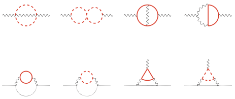
Figure 2: Sample two-loop diagrams that appear in the calculation of $\zeta_{\alpha_{2}}$. Red (bold) lines represent massive (scalar and fermionic) triplets and black (thin) lines massless fields. Furthermore, curly lines denote gauge bosons, dotted lines ghosts, dashed lines scalar fields and solid lines fermions.

V Numerical analysis

In this section we study the numerical impact of the newly computed corrections on the evolution of the gauge couplings and on the correlation function between the electroweak-triplet masses and the GUT scale. In practice, we integrate numerically the $n$-loop beta functions of the gauge couplings taking into account also the $(n-1)$-loop running of the top-Yukawa coupling and the $(n-2)$-loop running of the Higgs boson self-coupling. We can safely neglect the contribution of the bottom and tau Yukawa couplings and defer the study of the effect due to the new scalar self-interactions of the scalar triplet $T_{H}$ to Section V.1 (i.e. we set here $\alpha_{\lambda_{T}}=0$ and $\alpha_{\lambda_{hT}}=0$). As input parameters for the running analysis we take Mihaila:2012pz

$$\alpha_{1}^{\overline{\text{MS}}}(M_{Z}) =0.0169225\pm 0.0000039\,,$$ (26)

$$\alpha_{2}^{\overline{\text{MS}}}(M_{Z}) =0.033735\pm 0.000020\,,$$ (27)

$$\alpha_{3}^{\overline{\text{MS}}}(M_{Z}) =0.1173\pm 0.00069\,,$$ (28)

$$\alpha_{t}^{\overline{\text{MS}}}(M_{Z}) =0.07514\,,$$ (29)

given in the full SM, i.e. with the top quark threshold effects taken into account. The Higgs self-coupling in Eq. (10) is determined assuming a Higgs boson with mass $125$ GeV. Thus, we obtain

$$\alpha_{\lambda_{h}}\approx 0.010\,.$$ (30)

Let us start by studying the impact of the electroweak triplets on the running and decoupling of $\alpha_{2}$. When the decoupling is performed at the two-loop level the running masses must be consistently evolved at the one-loop order. At that order Eq. (23) can be easily integrated analytically yielding

$$m_{T_{F,H}}(\mu)=m_{T_{F,H}}(\mu_{0})\left(\frac{\alpha_{2}(\mu)}{\alpha_{2}(\mu_{0})}\right)^{-\frac{\pi}{\alpha_{2}a_{2}}\gamma^{(1-\rm{loop})}_{m_{T_{F,H}}}}\,,$$ (31)

where $a_{2}$ is the one-loop coefficient of the ${\rm SU(2)}_{L}$ gauge coupling beta function defined in Eq. (14), whereas $\gamma^{(1-\rm{loop})}_{m_{T_{F,H}}}$ are given in Eqs. (24)–(25). In the following we will drop for simplicity the scale dependence of the running masses. Unless otherwise specified the symbol “$m$” should be understood as $m(\mu=m)$.

In Fig. 3, we plot the gauge coupling $\alpha_{2}$ evolved until the reference scale of $10^{15}$ GeV as a function of the (unphysical) decoupling scale $\mu_{T}$ where the electroweak triplets are integrated out. We expect that the dependence on this unphysical parameter is reduced order by order in perturbation theory. Thus, we can use it as a measure of the convergence of the perturbation expansion. Indeed, from Fig. 3 we observe that the scale dependence is drastically reduced when the three-loop corrections are taken into account. Let us mention that the prediction obtained from the two-loop analysis for the “natural” choice of the decoupling scale $\mu_{T}=m_{3}$, where

$$m_{3}\equiv\left(m_{T_{F}}^{4}m_{T_{H}}\right)^{1/5}\,,$$ (32)

is usually within the experimental band of the three-loop result. For this choice of scale, discrepancies between the two- and three-loop predictions beyond the experimental accuracy are obtained only in the hierarchical case $m_{T_{H}}\ll m_{T_{F}}$.
Analogous considerations hold also for the effects of the colour-octet states $O_{F,H}$ on the running and decoupling of $\alpha_{3}$. However, the larger experimental uncertainty on $\alpha_{3}(M_{Z})$ always dominates over the theoretical mismatch between the two- and three-loop predictions.

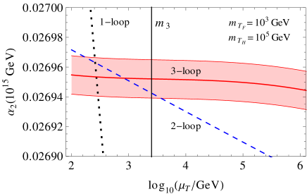
Figure 3: The value of the coupling $\alpha_{2}$ evaluated at the reference scale of $10^{15}\,\text{GeV}$ is shown as a function of the decoupling scale of the triplets $\mu_{T}$. Dotted (black), dashed (blue) and full (red) lines correspond respectively to the one-, two- and three-loop running analysis. The $1\sigma$ error band coming from the experimental value of $\alpha_{2}(M_{Z})$ is shown for the three-loop curve as well. The vertical (black) line denotes the quantity $m_{3}$ (cf. Eq. (32)), corresponding to the “naive” decoupling scale chosen in the two-loop analysis.

In Fig. 4 we show a sample three-loop unification pattern for the inverse of the gauge couplings and for the following choice of the intermediate-scale thresholds: $m_{T_{F}}=m_{T_{H}}=10^{2.5}\,\text{GeV}$, $m_{O_{F}}=m_{O_{H}}=10^{7.5}\,\text{GeV}$, $m_{X_{F}}=M_{G}/100$ and $m_{\mathcal{T}}=m_{X_{V}}=M_{G}$. Here $M_{G}$ is operatively defined as the scale at which $\alpha_{1}$, $\alpha_{2}$ and $\alpha_{3}$ meet, up to GUT-threshold corrections. The running and decoupling procedure is performed at the NNLO level (i.e. three-loop running and two-loop matching) with the exception of the short final stage of the running between $m_{X_{F}}$ and $M_{G}$ for which we consider the decoupling of $X_{F}$ and its contribution to the gauge coupling beta functions only at the one- Weinberg:1980wa ; Hall:1980kf and two-loop level Machacek:1983tz , respectively. Furthermore, the GUT-threshold corrections are considered only at one loop Weinberg:1980wa ; Hall:1980kf .

In order to quantify the impact of the newly computed corrections let us mention that for such a sample unification pattern the relative difference between the two- and three-loop values of $\alpha_{1}$, $\alpha_{2}$ and $\alpha_{3}$ evaluated at $M_{G}$ amounts to $0.015\%$, $0.061\%$ and $0.08\%$, respectively. This has to be compared with the relative experimental uncertainties: $\Delta\alpha_{1}/\alpha_{1}=0.023\%$, $\Delta\alpha_{2}/\alpha_{2}=0.059\%$ and $\Delta\alpha_{3}/\alpha_{3}=0.59\%$. Hence, for $\alpha_{1}$ and $\alpha_{2}$ the three-loop corrections are of the same order of magnitude as the experimental uncertainties, while for the case of $\alpha_{3}$ the experimental error dominates with respect to the theoretical one.

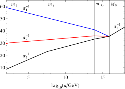
Figure 4: Sample three-loop unification pattern for $m_{T_{F}}=m_{T_{H}}=10^{2.5}\,\text{GeV}$, $m_{O_{F}}=m_{O_{H}}=10^{7.5}\,\text{GeV}$, $m_{X_{F}}=M_{G}/100$ and $m_{\mathcal{T}}=m_{X_{V}}=M_{G}$. The lines with different slopes from top to bottom correspond to $\alpha_{1}^{-1}$ (blue), $\alpha_{2}^{-1}$ (red) and $\alpha_{3}^{-1}$ (black). The dashed vertical lines denote the masses of the intermediate-scale thresholds, where $m_{3}$ is defined in Eq. (32) and $m_{8}$ is analogously defined as $m_{8}\equiv\left(m_{O_{F}}^{4}m_{O_{H}}\right)^{1/5}$.

In Fig. 5, the region of gauge coupling unification is enlarged. The inverse of the coupling constants $\alpha_{1},\alpha_{2}$ and $\alpha_{3}$ is shown together with the error bands induced by the experimental uncertainties on their values at the scale $M_{Z}$. From the figure it is evident that threshold effects at the GUT scale have to be taken into account for a proper unification.

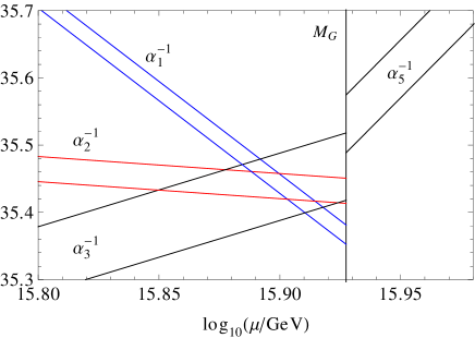
Figure 5: Detail of the three-loop unification pattern of Fig. 4 in the vicinity of the unification scale, including the $1\sigma$ error bands.

One of the most interesting observables of the present running analysis is the correlation between the effective electroweak-triplet mass $m_{3}$ (cf. Eq. (32)) and the unification scale $M_{G}$ Bajc:2006ia . Such a correlation mainly depends on the convergence scale of the couplings $\alpha_{1}$ and $\alpha_{2}$, whenever the masses of the super-heavy particles $X_{F}$ and $\mathcal{T}$ are fixed. The coupling $\alpha_{3}$ enters the correlation function only indirectly from the two-loop level on. Hence, for this particular observable, the uncertainty induced by $\alpha_{3}(M_{Z})$ remains always subleading wrt that caused by $\alpha_{1,2}(M_{Z})$. Moreover, also the colour-octet states $O_{F,H}$, that give sizable contributions only to the evolution of the strong coupling constant, have a minor role.
The predicted value for the couplings $\alpha_{1,2}$ at high energies maintains an exact dependence on $m_{3}$ at the one- and two-loop order (whenever the triplets are decoupled at the scale $\mu_{T}=m_{3}$) and remains approximate, usually within the experimental uncertainty, at the three-loop level.

The upper bound on the effective triplet mass $m_{3}$ is the crucial parameter for phenomenology Bajc:2006ia . For a fixed unification scale, $m_{3}^{\rm{max}}$ is obtained by maximizing the masses of the extra thresholds $X_{F}$ and $\mathcal{T}$. For a given choice of the cutoff $\Lambda$ of the SU(5) effective theory, namely $\Lambda=100\ M_{G}$ (cf. the discussion at the end of Section III), the masses of the electroweak triplets are maximized by taking $m_{X_{F}}=M_{G}/100$. For the colour-triplet scalar $\mathcal{T}$ the maximal allowed mass scale is in principle the Planck scale. However, the dependence of $m_{3}^{\rm{max}}$ on the colour-triplet mass turns out to be mild. For instance, varying the colour-triplet mass between the unification and the Planck scales induces a variation on the parameter $m_{3}^{\rm{max}}$ which lays within the experimental uncertainty. For convenience, we set the mass of the colour-triplet scalar to the unification scale $m_{\mathcal{T}}=M_{G}$. Here, $M_{G}$ is operatively defined as the scale where $\alpha_{1}$ and $\alpha_{2}$ meet up to corrections induced by the one-loop matching between the $\rm{SM+T+O+X_{F}}$ and the ${\rm SU(5)}+24_{F}$ theories. The size of these matching corrections can be read from Fig. 5. We also identify $M_{G}$ with the mass of the super-heavy gauge boson $X_{V}$ responsible for the gauge-induced proton decay rate.

In Fig. 6 we show $m_{3}^{\rm{max}}$ as a function of $M_{G}$ at the one-, two- and three-loop level, respectively. Notice that the two-loop correction on $m_{3}^{\rm{max}}$ for a fixed $M_{G}$ is of the same order of magnitude as the one-loop contribution and amounts to several TeV. On the other hand, the three-loop correction pushes the correlation only a bit up, but always within the experimental uncertainty of the two-loop band. Hence, the theoretical error due to the perturbative expansion (defined by the relative difference between the $n$- and the $(n-1)$-loop prediction) is reduced now at the same level as the experimental uncertainty induced by the measurement of $\alpha_{1}$ and $\alpha_{2}$ at the Z-boson mass scale. From Fig. 6 we can estimate that for a given unification scale $M_{G}$, the effective parameter $m_{3}^{\rm{max}}$ can be now determined with a $25\%$ accuracy.

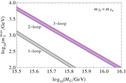
Figure 6: The maximal value of the effective triplet mass $m_{3}$ as a function of the unification scale $M_{G}$. The black, blue and red bands (from bottom-left to top-right) correspond respectively to the one-, two- and three-loop running analysis. The three-loop result is obtained by taking $m_{T_{F}}=m_{T_{H}}$. The error bands are due to the $1\sigma$ uncertainties on the low-energy couplings $\alpha_{1}(M_{Z})$ and $\alpha_{2}(M_{Z})$ (cf. Eqs. (26)–(27)).

It is worth mentioning that starting from three loops the $m^{\rm{max}}_{3}-M_{G}$ correlation shows also a dependence on the ratio $m_{T_{F}}/m_{T_{H}}$. In particular, larger deviations between the two- and three-loop analysis are observed for the case when $m_{T_{H}}\ll m_{T_{F}}$. However, for the mass range relevant for unification, the three-loop corrections to the correlation function $m^{\rm{max}}_{3}-M_{G}$ for $m_{T_{H}}\neq m_{T_{F}}$ turn out to be always within the experimental uncertainty of the two-loop prediction. For illustration, we show in Fig. 7 $M_{G}$ as a function of the $m_{T_{F}}/m_{T_{H}}$ ratio for a fixed value of $m_{3}^{\rm{max}}$.

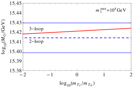
Figure 7: $M_{G}$ as a function of the $m_{T_{F}}/m_{T_{H}}$ ratio for a fixed value of $m_{3}^{\rm{max}}$. The dashed (blue) and full (red) lines correspond respectively to the two- and three-loop running analysis. The $1\sigma$ error band is shown as well for the two-loop case. The negative and positive extrema on the x-axis correspond respectively to the configurations $m_{T_{F}}=10^{3.6}\ \text{GeV}$, $m_{T_{H}}=10^{5.6}\ \text{GeV}$ and $m_{T_{F}}=10^{4.4}\ \text{GeV}$, $m_{T_{H}}=10^{2.4}\ \text{GeV}$.

Finally, the analysis of the full unification pattern, including the convergence of $\alpha_{3}$ with $\alpha_{1,2}$, fixes the masses of the colour octets $O_{F,H}$ in terms of the other masses of the model (see the discussion in Ref. Bajc:2006ia ; Bajc:2007zf ). However, the newly computed corrections induced by the colour-octet states to the two-loop matching coefficient and three-loop beta function of $\alpha_{3}$ (cf. Appendix B) are subleading as compared to the experimental uncertainty on $\alpha_{3}(M_{Z})$. A two-loop analysis as in Bajc:2006ia ; Bajc:2007zf is usually sufficient.

V.1 Scalar self-interactions

At the tree-loop level all the sectors of the theory enter for the first time into the running of the gauge couplings. In particular, this is also true for the couplings $\alpha_{\lambda_{h}}$, $\alpha_{\lambda_{T}}$ and $\alpha_{\lambda_{hT}}$ of the scalar potential in Eq. (10). However, while $\alpha_{\lambda_{h}}$ is fixed in terms of the SM Higgs boson mass (cf. Eq. (30)), $\alpha_{\lambda_{T}}$ and $\alpha_{\lambda_{hT}}$ are essentially unconstrained and could, if large enough, contribute significantly to the running of the gauge couplings after $T_{H}$ is integrated in.

In order to quantify how large the scalar self-couplings can be, let us inspect their one-loop beta functions Forshaw:2003kh

$$\pi^{2}\beta_{\alpha_{\lambda_{h}}} =3\alpha_{\lambda_{h}}^{2}+\frac{3}{2}\alpha_{\lambda_{h}}\alpha_{t}+\frac{3}{4}\alpha_{\lambda_{hT}}^{2}-\frac{3}{4}\alpha_{t}^{2}\,,$$ (33)

$$\pi^{2}\beta_{\alpha_{\lambda_{T}}} =\frac{11}{2}\alpha_{\lambda_{T}}^{2}+\frac{1}{2}\alpha_{\lambda_{hT}}^{2}\,,$$ (34)

$$\pi^{2}\beta_{\alpha_{\lambda_{hT}}} =\alpha_{\lambda_{hT}}^{2}+\left(\frac{3}{2}\alpha_{\lambda_{h}}+\frac{5}{2}\alpha_{\lambda_{T}}+\frac{3}{4}\alpha_{t}\right)\alpha_{\lambda_{hT}}\,,$$ (35)

where we considered for simplicity the gauge-less limit $(\alpha_{1,2}\rightarrow 0)$ and retained only the top-Yukawa contribution $\alpha_{t}$. The definition of the beta functions follows the conventions in Eq. (14).

Eqs. (33)–(35) show that for large and positive initial values of the couplings $\alpha_{\lambda_{T}}$ and $\alpha_{\lambda_{hT}}$ the renormalization group evolution is such that all the scalar self-couplings can easily become nonperturbative below $M_{G}$. In such a situation perturbation theory breaks down, meaning that we cannot trust our predictions about gauge coupling unification. Imposing the conservative bound $\alpha_{\lambda_{T},\lambda_{hT}}<0.01$ we have checked that Landau poles are not developed below $M_{G}$ and the effects on the $m_{3}^{\rm{max}}-M_{G}$ correlation are always within the experimental band of the two-loop analysis.

VI Conclusions and outlook

In this work we have undertaken an important step towards the study of gauge coupling unification in the ${\rm SU(5)}+24_{F}$ model Bajc:2006ia ; Bajc:2007zf at the three-loop level. We computed the contributions of the electroweak triplets $T_{F,H}$ and the colour octets $O_{F,H}$ (which are predicted to be well below the GUT scale in this specific model) to the three-loop beta functions and the two-loop matching coefficients of the SM gauge couplings.

In particular, the most important observable of the running analysis is the correlation between the maximal value of an effective triplet mass parameter $m^{\rm{max}}_{3}$ and the unification scale $M_{G}$. This correlation is shown in Fig. 6 and is such that the electroweak triplets can escape the detection at LHC only if the unification scale is below $\approx 10^{16}$ GeV, thus implying a proton lifetime which should be accessible to the future generation of megaton-scale proton decay experiments Abe:2011ts .
Such a correlation needs to be computed as accurately as possible. Indeed, for a fixed value of $M_{G}$, the parameter $m^{\rm{max}}_{3}$ can be in principle extracted from the low-energy values of $\alpha_{1}$ and $\alpha_{2}$ with an accuracy of about $25\%$. On the other hand, for a fixed value of $M_{G}$, the values of $m^{\rm{max}}_{3}$ predicted at one and two loops differ by around $100\%$ (cf. again Fig. 6). Hence, for this particular observable which is almost insensitive to the low-energy value of $\alpha_{3}$, the three-loop corrections are required in order to settle the accuracy of the theoretical prediction at the level of the experimental precision.

Still, one should keep in mind the existence of irreducible theoretical uncertainties which plague any GUT and may endanger the predictivity of a given scheme. These are, for instance, the presence of effective operators which are required either by the self-consistency of the theory (as in the ${\rm SU(5)}+24_{F}$ model) or which are expected on physical grounds due to the vicinity of the Planck and the GUT scales. In this sense, an effort towards a three-loop analysis of gauge coupling unification should be minimally understood as a way to reduce the theoretical error due to the perturbative expansion.

However, the path towards a complete three-loop analysis of gauge coupling unification in GUTs (with or without supersymmetry) is still long and many important ingredients are still missing. These are, for instance, the contributions to the three-loop beta functions and the two-loop matching coefficients of arbitrary multiplets charged under the SM group. Intermediate-mass scale multiplets are usually predicted in nonsupersymmetric GUTs and the knowledge of a general formula for their contribution could allow to extend the study of gauge coupling unification at the three-loop level also to other well motivated scenarios based on SU(5) Dorsner:2005fq ; *Dorsner:2005ii; Perez:2007rm ; Dorsner:2007fy ; Feldmann:2010yp and SO(10) Bertolini:2013vta ; *Bertolini:2012im; *Bertolini:2009es. Finally, the last important and conceptually challenging ingredient is represented by the two-loop matching at the GUT scale. In this respect, a step towards such a calculation has already been performed in the context of the GG SU(5) model Martens:2010pe and could be in principle extended both to nonsupersymmetric and supersymmetric GUTs.

Acknowledgments

We thank Borut Bajc, Miha Nemevšek and Goran Senjanović for their interest in this project and for useful discussions. This work was supported by the DFG through the SFB/TR 9 “Computational Particle Physics”.

Appendix A Details of the SU(5) + ${\bf 24_{F}}$ model

In this appendix we collect some basic facts about the SU(5) model augmented with a fermionic $24_{F}$ multiplet. In particular, we recompute the mass spectrum and derive the low-energy interactions among the SM fields and the remnant GUT states which populate the desert at intermediate mass scales. The latter motivate the interactions included into the three-loop analysis computation.

A.1 Field content and SM embedding

The field content of the model features an additional $24_{F}$ on top of the original representations of the GG model, namely three copies of $\overline{5}_{F}\oplus 10_{F}$ and $5_{H}\oplus 24_{H}$ in the Higgs sector. The embedding of the SM fields into the SU(5) representations is symbolically displayed in Section II. More precisely, spanning the SU(5), ${\rm SU(3)}_{C}$ and ${\rm SU(2)}_{L}$ spaces respectively with latin ($a=1,\ldots,5$), greek ($\alpha=1,\ldots,3$) and capital-latin ($A=1,2$) letters, we have

$$(5_{H})_{a}=\left(\begin{array}[]{c}\mathcal{T}_{\alpha}\\ h_{A}\end{array}\right)\,,\qquad(\overline{5}_{F})^{a}=\left(\begin{array}[]{c}d^{c\alpha}\\ \epsilon^{AB}\ell_{B}\end{array}\right)\,,$$ (36)

$$(\overline{10}_{F})_{ab}=\tfrac{1}{\sqrt{2}}\left(\begin{array}[]{cc}\epsilon_{\alpha\beta\gamma}u^{c\gamma}&-q_{\alpha B}\\ q_{A\beta}&\epsilon_{AB}e^{c}\end{array}\right)\,,$$ (37)

where the completely antisymmetric tensors in the ${\rm SU(2)}_{L}$ and ${\rm SU(3)}_{C}$ spaces are defined so that $\epsilon^{12}=1$ and $\epsilon_{123}=1$, and

$$(24_{H,F,V})^{\ b}_{a}=\mathcal{N}_{H,F,V}\\ \left(\begin{array}[]{cc}(O_{H,F,V})^{\ \beta}_{\alpha}+\tfrac{2}{\sqrt{30}}S_{H,F,V}\delta^{\ \beta}_{\alpha}&(X_{H,F,V})^{\ B}_{\alpha}\\ (\overline{X}_{H,F,V})^{\ A}_{\beta}&(T_{H,F,V})^{\ B}_{A}-\tfrac{3}{\sqrt{30}}S_{H,F,V}\delta^{\ B}_{A}\end{array}\right)\,,$$ (38)

where we defined the quantities

$$O^{\ \beta}_{\alpha}=\tfrac{1}{\sqrt{2}}O^{i}(\lambda_{i})^{\ \beta}_{\alpha}\quad\text{and}\quad T^{\ B}_{A}=\tfrac{1}{\sqrt{2}}T^{i}(\sigma_{i})^{\ B}_{A}$$ (39)

with $\lambda_{i}$ ($i=1,\ldots,8$) and $\sigma_{i}$ ($i=1,\ldots,3$) denoting respectively the Gell-Mann and Pauli matrices normalized as $\mbox{Tr}\,\lambda_{i}\lambda_{j}=2\delta_{ij}$ and $\mbox{Tr}\,\sigma_{i}\sigma_{j}=2\delta_{ij}$. So, in particular, we have $\mbox{Tr}\,T^{2}=T^{i}T^{i}\equiv\left|T\right|^{2}$ and $\mbox{Tr}\,O^{2}=O^{i}O^{i}\equiv\left|O\right|^{2}$. $\mathcal{N}_{H,F,V}$ is a normalization factor equal to $1$ ($H$) and $\tfrac{1}{\sqrt{2}}$ ($F,V$) respectively.

A.2 Mass spectrum

The calculation of the tree-level mass spectrum allows to address the important question whether the states required by the unification pattern can be consistently fine-tuned at the corresponding intermediate mass scales. For completeness we report it here, though it can be partially found also elsewhere (see for instance Refs. Buras:1977yy ; Bajc:2006ia ; Bajc:2007zf ).

A.2.1 Scalar sector

The scalar sector consists in the potential for the GUT-breaking field $24_{H}$

$$V_{24_{H}}=m^{2}_{24}\mbox{Tr}\,24_{H}^{2}+\mu_{24}\mbox{Tr}\,24_{H}^{3}\\ +\lambda^{(1)}_{24}\mbox{Tr}\,24_{H}^{4}+\lambda^{(2)}_{24}\left(\mbox{Tr}\,24_{H}^{2}\right)^{2}$$ (40)

and its interaction with the $5_{H}$,

$$V_{5_{H}}=m^{2}_{H}5_{H}^{\dagger}5_{H}+\lambda_{H}(5_{H}^{\dagger}5_{H})^{2}+\mu_{H}5_{H}^{\dagger}24_{H}5_{H}\\ +\alpha\,5_{H}^{\dagger}5_{H}\mbox{Tr}\,24_{H}^{2}+\beta\,5_{H}^{\dagger}24_{H}^{2}5_{H}\,.$$ (41)

SU(5) is spontaneously broken to the SM by

$$\left\langle 24_{H}\right\rangle=\frac{V}{\sqrt{30}}\rm{diag}(2,2,2,-3,-3)\,,$$ (42)

where $V$ is a vacuum expectation value in the SM-singlet direction $\left\langle S_{H}\right\rangle$ (cf. Eq. (38)). By substituting Eq. (42) into Eq. (40) the vacuum manifold reads

$$\left\langle V_{24_{H}}\right\rangle=m^{2}_{24}V^{2}-\frac{\mu_{24}}{\sqrt{30}}V^{3}+\left(\tfrac{7}{30}\lambda^{(1)}_{24}+\lambda^{(2)}_{24}\right)V^{4}$$ (43)

and the corresponding stationary equation for $V\neq 0$ can be conveniently written as

$$0=\frac{1}{V}\frac{d\left\langle V_{24_{H}}\right\rangle}{dV}=\\ 2m^{2}_{24}-\sqrt{\tfrac{3}{10}}\mu_{24}V+\left(\tfrac{14}{15}\lambda^{(1)}_{24}+4\lambda^{(2)}_{24}\right)V^{2}\,.$$ (44)

The scalar spectrum is readily obtained by expanding the scalar potential around the SM-invariant vacuum configuration in Eq. (42). After trading $m^{2}_{24}$ by means of the stationary condition in Eq. (44), this yields

$$m^{2}_{S_{H}}=-\sqrt{\tfrac{3}{10}}\mu_{24}V+4\left(\tfrac{7}{15}\lambda^{(1)}_{24}+2\lambda^{(2)}_{24}\right)V^{2}\,,$$ (45)

$$m^{2}_{T_{H}}=-\sqrt{\tfrac{15}{2}}\mu_{24}V+\tfrac{8}{3}\lambda^{(1)}_{24}V^{2}\,,$$ (46)

$$m^{2}_{O_{H}}=+\sqrt{\tfrac{15}{2}}\mu_{24}V+\tfrac{2}{3}\lambda^{(1)}_{24}V^{2}\,,$$ (47)

$$m^{2}_{X_{H}}=0\,,$$ (48)

with the zero modes corresponding to the would-be Goldstone bosons giving mass to the longitudinal components of $X_{V}$. The tree-level vacuum stability (cf. Eq. (43)) implies

$$\tfrac{7}{30}\lambda^{(1)}_{24}+\lambda^{(2)}_{24}>0\,,$$ (49)

while, requiring that the scalar masses in Eqs. (45)–(47) are positive definite (minimum condition) gives

$$\lambda^{(1)}_{24}>0\,,\quad-\tfrac{2}{3}\sqrt{\tfrac{2}{15}}\lambda^{(1)}_{24}<\mu_{24}/V<\tfrac{8}{3}\sqrt{\tfrac{2}{15}}\lambda^{(1)}_{24}\,,$$ (50)

and

$$\lambda^{(2)}_{24}>-\tfrac{7}{30}\lambda^{(1)}_{24}+\tfrac{1}{8}\sqrt{\tfrac{3}{10}}\mu_{24}/V\,.$$ (51)

Since the unification constraints favor a rather light $T_{H}$ it is interesting to work out the vacuum conditions in the limit $m^{2}_{T_{H}}\approx 0$. In the latter case the heavy spectrum reads

$$m^{2}_{S_{H}}\approx\left(\tfrac{4}{3}\lambda^{(1)}_{24}+8\lambda^{(2)}_{24}\right)V^{2}\,,$$ (52)

$$m^{2}_{O_{H}}\approx\tfrac{10}{3}\lambda^{(1)}_{24}V^{2}\,,$$ (53)

and the absence of tachyons in the scalar spectrum enforces

$$\lambda^{(1)}_{24}>0\qquad\text{and}\qquad\lambda^{(2)}_{24}>-\tfrac{1}{6}\lambda^{(1)}_{24}\,,$$ (54)

which automatically satisfies also the tree-level vacuum stability condition in Eq. (49). Notice that a small (positive) value of $\lambda^{(1)}_{24}$ allows to consistently keep also the mass of $O_{H}$ below the GUT scale.

Finally, by plugging the SM-invariant vacuum configuration of Eq. (42) into Eq. (41) we get the spectrum of the fields residing in $5_{H}$, which reads

$$m^{2}_{\mathcal{T}}=m^{2}_{H}+\sqrt{\tfrac{2}{15}}\mu_{H}V+\left(\alpha+\tfrac{2}{15}\beta\right)V^{2}\,,$$ (55)

$$m^{2}_{h}=m^{2}_{H}-\sqrt{\tfrac{3}{10}}\mu_{H}V+\left(\alpha+\tfrac{3}{10}\beta\right)V^{2}\,.$$ (56)

Therefore it is possible to perform the standard doublet-triplet splitting $m^{2}_{h}\approx 0$, which yields in turn

$$m^{2}_{\mathcal{T}}\approx\sqrt{\tfrac{5}{6}}\mu_{H}V-\tfrac{1}{6}\beta V^{2}\,.$$ (57)

A.2.2 Yukawa sector

On top of the usual Yukawa sector responsible for the masses of the charged fermions

$$\mathcal{L}_{Ycf}=y_{ij}\overline{5}_{F}^{i}10_{F}^{j}5_{H}^{*}+h_{ij}10_{F}^{i}10_{F}^{j}5_{H}+\rm{h.c.}+\ldots\,,$$ (58)

where the ellipses stand for nonrenormalizable operators needed to reproduce the correct mass ratios between down-quarks and charged-leptons (see e.g. Ellis:1979fg ; Dorsner:2006hw ), we add the new Yukawa interactions Bajc:2006ia ; Bajc:2007zf

$$\mathcal{L}_{Y\nu}=y^{i}_{0}\overline{5}_{F}^{i}24_{F}5_{H}+\frac{1}{\Lambda}\overline{5}_{F}^{i}\left(y^{i}_{1}24_{F}24_{H}\right.\\ \left.+y^{i}_{2}24_{H}24_{F}+y^{i}_{3}\mbox{Tr}\,(24_{F}24_{H})\right)5_{H}+\rm{h.c.}\,,$$ (59)

where $\Lambda$ denotes the cutoff of the effective theory. After SU(5) breaking Eq. (59) yields

$$\mathcal{L}_{Y\nu}\ni\ell_{i}^{T}(i\sigma_{2})^{T}\left(y^{i}_{T}T_{F}+y^{i}_{S}S_{F}\right)h+\rm{h.c.}\,,$$ (60)

where $y^{i}_{T}$ and $y^{i}_{S}$ are two different linear combinations of $y_{0}^{i}$ and $y_{a}^{i}V/\Lambda$ ($a=1,2,3$), namely

$$y^{i}_{T}=\tfrac{1}{\sqrt{2}}y_{0}^{i}-\tfrac{1}{2}\sqrt{\tfrac{3}{5}}(y^{i}_{1}+y^{i}_{2})\frac{V}{\Lambda}\,,$$ (61)

$$y^{i}_{S}=-\sqrt{\tfrac{3}{10}}y^{i}_{T}+\tfrac{1}{\sqrt{2}}y^{i}_{3}\frac{V}{\Lambda}\,.$$ (62)

In particular, the coupling $y^{i}_{3}$ is responsible for the misalignment of the vectors $y^{i}_{T}$ and $y^{i}_{S}$ in the flavour space, thus leading to a rank-2 neutrino mass matrix when integrating out the heavy vector-like states $T_{F}$ and $S_{F}$:

$$m^{\nu}_{ij}=-\frac{v^{2}}{2}\left(\frac{y_{T}^{i}y_{T}^{j}}{m_{T_{F}}}+\frac{y_{S}^{i}y_{S}^{j}}{m_{S_{F}}}\right)\,.$$ (63)

Instead, the masses of the new fermions residing in $24_{F}$ are due to the Yukawa-like interactions Bajc:2006ia ; Bajc:2007zf

$$\mathcal{L}_{F} =m_{F}\mbox{Tr}\,24_{F}^{2}+\lambda_{F}\mbox{Tr}\,24_{F}^{2}24_{H}$$

$$+\frac{1}{\Lambda}\left(a_{1}\mbox{Tr}\,24_{F}^{2}\mbox{Tr}\,24_{H}^{2}+a_{2}\mbox{Tr}\,(24_{F}24_{H})^{2}\right.$$

$$+\left.a_{3}\mbox{Tr}\,24_{F}^{2}24_{H}^{2}+a_{4}\mbox{Tr}\,24_{F}24_{H}24_{F}24_{H}\right)\,,$$ (64)

which, after SU(5) breaking, lead to the following spectrum:

$$m_{S_{F}}=m_{F}-\tfrac{1}{\sqrt{30}}\lambda_{F}V+\left(a_{1}+a_{2}+\tfrac{7}{30}(a_{3}+a_{4})\right)\frac{V^{2}}{\Lambda}\,,$$ (65)

$$\!\!\!\!m_{T_{F}}=m_{F}-\sqrt{\tfrac{3}{10}}\lambda_{F}V+\left(a_{1}+\tfrac{3}{10}(a_{3}+a_{4})\right)\frac{V^{2}}{\Lambda}\,,$$ (66)

$$\!\!\!\!m_{O_{F}}=m_{F}+\tfrac{2}{\sqrt{30}}\lambda_{F}V+\left(a_{1}+\tfrac{2}{15}(a_{3}+a_{4})\right)\frac{V^{2}}{\Lambda}\,,$$ (67)

$$\!\!\!\!m_{X_{F}}=m_{F}-\tfrac{1}{2\sqrt{30}}\lambda_{F}V+\left(a_{1}+\tfrac{13}{60}a_{3}-\tfrac{1}{5}a_{4}\right)\frac{V^{2}}{\Lambda}\,.$$ (68)

Since unification constraints require a light $T_{F}$, we must impose $m_{T_{F}}\approx 0$. In turn, the spectrum of the other fields residing in $24_{F}$ becomes

$$m_{S_{F}} \approx\sqrt{\tfrac{2}{15}}\lambda_{F}V+\left(a_{2}-\tfrac{1}{15}(a_{3}+a_{4})\right)\frac{V^{2}}{\Lambda}\,,$$ (69)

$$m_{O_{F}} \approx\sqrt{\tfrac{5}{6}}\lambda_{F}V-\tfrac{1}{6}(a_{3}+a_{4})\frac{V^{2}}{\Lambda}\,,$$ (70)

$$m_{X_{F}} \approx\tfrac{1}{2}\sqrt{\tfrac{5}{6}}\lambda_{F}V-\tfrac{1}{2}(\tfrac{1}{6}a_{3}+a_{4})\frac{V^{2}}{\Lambda}\,.$$ (71)

Further requiring an intermediate-scale octet ($m_{O_{F}}\approx 0$), one gets

$$m_{S_{F}} \approx a_{2}\frac{V^{2}}{\Lambda}\,,$$ (72)

$$m_{X_{F}} \approx-\tfrac{5}{12}a_{4}\frac{V^{2}}{\Lambda}\,,$$ (73)

which shows that the upper bound on the mass of the $X_{F}$ state is of order $V^{2}/\Lambda$.

A.2.3 Gauge sector

The gauge boson masses are obtained from the canonical kinetic term

$$\tfrac{1}{2}\,\mbox{Tr}\,\left(D_{\mu}\left\langle 24_{H}\right\rangle\right)^{\dagger}D^{\mu}\left\langle 24_{H}\right\rangle\,,$$ (74)

where $D_{\mu}$ is the SU(5) covariant derivative

$$D_{\mu}24_{H}=\partial_{\mu}24_{H}+ig_{5}\left[(24_{V})_{\mu},24_{H}\right]\,.$$ (75)

After plugging into Eq. (74) the expression for $\left\langle 24_{H}\right\rangle$ (cf. Eq. (42)), one finds

$$m^{2}_{S_{V}}=m^{2}_{T_{V}}=m^{2}_{O_{V}}=0\ \ \ \text{and}\ \ \ m^{2}_{X_{V}}=\tfrac{5}{12}g_{5}^{2}V^{2}\,,$$ (76)

leading to the 12 massless modes of the SM gauge bosons, plus the 12 degrees of freedom of the super-heavy gauge boson $X_{V}$.

A.3 Low-energy interactions

Here we derive the interactions in the low-energy effective theory featuring the SM fields and the five intermediate mass-scale states $S_{F}$, $T_{F}$, $O_{F}$, $T_{H}$ and $O_{H}$.

Let us start from the Yukawa-like interactions. At the leading order in $V/\Lambda$ we find

$$\mathcal{L}_{F}\ni y_{STT}\,S_{F}\,\mbox{Tr}\,T_{F}T_{H}\\ +y_{SOO}\,S_{F}\,\mbox{Tr}\,O_{F}O_{H}+y_{OOO}\,\mbox{Tr}\,O_{F}^{2}O_{H}\,,$$ (77)

with $O_{H,F}$ and $T_{H,F}$ defined in Eq. (39) and

$$y_{STT}=-\sqrt{\tfrac{3}{10}}\lambda_{F}+\left(a_{2}+\tfrac{3}{5}(a_{3}+a_{4})\right)\frac{V}{\Lambda}\,,$$ (78)

$$y_{SOO}=\sqrt{\tfrac{2}{15}}\lambda_{F}+\left(a_{2}+\tfrac{4}{15}(a_{3}+a_{4})\right)\frac{V}{\Lambda}\,,$$ (79)

$$y_{OOO}=\tfrac{1}{2}\lambda_{F}+\sqrt{\tfrac{2}{15}}(a_{3}+a_{4})\frac{V}{\Lambda}\,.$$ (80)

Notice that the ${\rm SU(2)}_{L}$ invariant $\mbox{Tr}\,T_{F}^{2}T_{H}$ is zero by antisymmetry.

The couplings $y_{STT}$, $y_{SOO}$ and $y_{OOO}$ have an upper bound of $\mathcal{O}\left(V/\Lambda\right)$, since the unification pattern requires a splitting among the masses in Eqs. (65)–(68). In particular, for light $T_{F}$ and $O_{F}$ they reduce to

$$y_{STT}\approx\left(a_{2}+\tfrac{1}{2}(a_{3}+a_{4})\right)\frac{V}{\Lambda}\,,$$ (81)

$$y_{SOO}\approx\left(a_{2}+\tfrac{1}{3}(a_{3}+a_{4})\right)\frac{V}{\Lambda}\,,$$ (82)

$$y_{OOO}\approx\tfrac{1}{2}\sqrt{\tfrac{5}{6}}(a_{3}+a_{4})\frac{V}{\Lambda}\,.$$ (83)

The other interactions relevant for the scalar sector are

$$V_{24_{H}}\ni\mu_{O}\,\mbox{Tr}\,O_{H}^{3}+\tfrac{\lambda_{T}}{2}\left(\mbox{Tr}\,T_{H}^{2}\right)^{2}\\ +\lambda_{TO}\,\mbox{Tr}\,T_{H}^{2}\,\mbox{Tr}\,O_{H}^{2}+\lambda_{O}\left(\mbox{Tr}\,O_{H}^{2}\right)^{2}\,,$$ (84)

where

$$\mu_{O}=\mu_{24}+4\sqrt{\tfrac{2}{15}}V\lambda^{(1)}_{24}\,,$$ (85)

$$\lambda_{T}=\lambda^{(1)}_{24}+2\lambda^{(2)}_{24}\,,$$ (86)

$$\lambda_{TO}=2\lambda^{(2)}_{24}\,,$$ (87)

$$\lambda_{O}=\tfrac{1}{2}\lambda^{(1)}_{24}+\lambda^{(2)}_{24}\,.$$ (88)

Notice that the ${\rm SU(2)}_{L}$ invariant $\mbox{Tr}\,T_{H}^{3}$ is zero by antisymmetry and that we also used the relations $\mbox{Tr}\,T_{H}^{4}=\tfrac{1}{2}(\mbox{Tr}\,T_{H}^{2})^{2}$ and $\mbox{Tr}\,O_{H}^{4}=\tfrac{1}{2}(\mbox{Tr}\,O_{H}^{2})^{2}$.

In particular, in the limit of a light $T_{H}$ (cf. Eq. (46)), we have

$$\mu_{O}\approx\tfrac{4}{3}\sqrt{\tfrac{10}{3}}V\lambda^{(1)}_{24}\,.$$ (89)

When also $O_{H}$ is below the GUT scale, $\lambda^{(1)}_{24}\approx 0$ (cf. Eq. (53)), which implies

$$\lambda_{T}\approx\lambda_{TO}\approx 2\lambda_{O}\,.$$ (90)

Finally, for the scalar interactions of the SM Higgs doublet, $h$, we obtain

$$V_{5_{H}}\ni\mu_{hT}\,h^{\dagger}T_{H}h+\lambda_{h}(h^{\dagger}h)^{2}\\ +\lambda_{hT}\,h^{\dagger}h\,\mbox{Tr}\,T_{H}^{2}+\lambda_{hO}\,h^{\dagger}h\,\mbox{Tr}\,O_{H}^{2}\,,$$ (91)

where

$$\mu_{hT}=\mu_{H}-\sqrt{\tfrac{6}{5}}V\beta\,,$$ (92)

$$\lambda_{h}=\lambda_{H}\,,$$ (93)

$$\lambda_{hT}=\alpha+\tfrac{1}{2}\beta\,,$$ (94)

$$\lambda_{hO}=\alpha\,,$$ (95)

and the relation $h^{\dagger}T_{H}^{2}h=\tfrac{1}{2}h^{\dagger}h\,\mbox{Tr}\,T_{H}^{2}$ has been also employed.

Among the couplings in Eqs. (85)–(88) and Eqs. (92)–(95) only $\lambda_{h}$ is fixed in terms of the Higgs boson mass, while the UV constraints coming from the SU(5) symmetry reduce only partially the allowed parameter space. On the other hand, an important constraint for the scalar parameters is given by the requirement of perturbativity (cf. the analysis in Section V.1).

Appendix B Further analytical results

In this Appendix we present the three-loop beta functions and the two-loop matching coefficients obtained by including the contribution of the colour octets.

B.1 Octet contribution to the beta functions

The pure-gauge contribution of the colour octets to the gauge coupling beta functions can be read from Eqs. (IV.1)–(20) after taking into account the proper substitutions:

• $\alpha_{2}\leftrightarrow\alpha_{3}$, $G_{L}\leftrightarrow G_{C}$, $R_{L}\leftrightarrow R_{C}$, $N_{h}\rightarrow 0$, $Y_{f}^{2}N_{f}\leftrightarrow Y_{Q}^{2}N_{Q}$ and $T_{F,H}\rightarrow O_{F,H}$ in Eq. (IV.1)

  $$\beta_{1}^{\rm SM+T+O}=\beta_{1}^{\rm SM+T}+\frac{\alpha_{1}^{2}}{\pi^{2}}\frac{\alpha_{3}^{2}}{\pi^{2}}C_{G_{C}}C_{R_{C}}N_{R_{C}}Y_{Q}^{2}N_{Q}\\ \times\left(-\frac{11}{576}{N_{O_{F}}}-\frac{23}{2304}{N_{O_{H}}}\right)\,,$$ (96)

• $\alpha_{2}\leftrightarrow\alpha_{3}$, $G_{L}\leftrightarrow G_{C}$, $R_{L}\leftrightarrow R_{C}$ and $T_{F,H}\rightarrow O_{F,H}$ in Eq. (20)

  $$\beta_{2}^{\rm SM+T+O}=\beta_{2}^{\rm SM+T}+\frac{\alpha_{2}^{2}}{\pi^{2}}\frac{\alpha_{3}^{2}}{\pi^{2}}C_{G_{C}}C_{R_{C}}N_{R_{C}}T_{R_{L}}N_{q}\\ \times\left(-\frac{11}{576}{N_{O_{F}}}-\frac{23}{2304}{N_{O_{H}}}\right)\,,$$ (97)

• $\alpha_{2}\leftrightarrow\alpha_{3}$, $G_{L}\leftrightarrow G_{C}$, $R_{L}\leftrightarrow R_{C}$, $N_{h}\rightarrow 0$, $N_{f}\leftrightarrow N_{Q}$ and $T_{F,H}\rightarrow O_{F,H}$ in Eq. (IV.1)

  $$\beta_{3}^{\rm SM+T+O} =\beta_{3}^{\rm SM+T}+\frac{\alpha_{3}^{2}}{\pi^{2}}\left\{C_{G_{C}}\left(\frac{1}{6}{N_{O_{F}}}+\frac{1}{24}{N_{O_{H}}}\right)+\frac{\alpha_{3}}{\pi}C_{G_{C}}^{2}\left(\frac{1}{3}{N_{O_{F}}}+\frac{7}{48}{N_{O_{H}}}\right)\right.$$

  $$+\frac{\alpha_{3}^{2}}{\pi^{2}}\left[\left(\frac{247}{432}C_{G_{C}}^{3}-\frac{7}{108}C_{G_{C}}^{2}T_{R_{C}}N_{Q}\right.\right.$$

  $$\left.-\frac{11}{576}C_{G_{C}}C_{R_{C}}T_{R_{C}}N_{Q}-\frac{145}{3456}C_{G_{C}}^{3}{N_{O_{F}}}-\frac{277}{6912}C_{G_{C}}^{3}{N_{O_{H}}}\right){N_{O_{F}}}$$

  $$+\left(\frac{2749}{6912}C_{G_{C}}^{3}-\frac{13}{432}C_{G_{C}}^{2}T_{R_{C}}N_{Q}\right.$$

  $$\left.\left.\left.-\frac{23}{2304}C_{G_{C}}^{2}C_{R_{C}}T_{R_{C}}N_{Q}-\frac{145}{13824}C_{G_{C}}^{3}{N_{O_{H}}}\right){N_{O_{H}}}\right]\right\}\,,$$ (98)

where we used the abbreviations: $Y_{Q}^{2}N_{Q}=N_{R_{L}}Y_{q}^{2}N_{q}+Y_{u}^{2}N_{u}+Y_{d}^{2}N_{d}$ and $N_{Q}=N_{R_{L}}N_{q}+N_{u}+N_{d}$. The numerical values of the beta functions specified to the SM+T+O model are obtained by the following replacements: (i) $Y_{q}=\sqrt{\tfrac{3}{5}}\tfrac{1}{6}$, $Y_{u}=-\sqrt{\tfrac{3}{5}}\tfrac{2}{3}$ and $Y_{d}=\sqrt{\tfrac{3}{5}}\tfrac{1}{3}$, denoting the hypercharges of the SM quarks in the SU(5) normalization; (ii) $N_{q}=N_{u}=N_{d}=3$ and $N_{O_{F,H}}=1$ standing for the number of SM quark generations, and colour octets.

B.2 Octet contribution to the matching coefficients

Considering again only the pure-gauge part, the color-octet contribution to the matching coefficient $\zeta_{\alpha_{3}}$ is obtained from Eq. (IV.2) after the following substitutions: $\alpha_{2}\leftrightarrow\alpha_{3}$, $G_{L}\leftrightarrow G_{C}$ and $T_{H,F}\leftrightarrow O_{H,F}$. These yield in turn

$$\zeta_{\alpha_{3}} =1+\frac{\alpha_{3}}{\pi}C_{G_{C}}\left(-\frac{1}{6}\ln{\frac{\mu^{2}}{m_{O_{F}}^{2}}}{N_{O_{F}}}-\frac{1}{24}\ln{\frac{\mu^{2}}{m_{O_{H}}^{2}}}{N_{O_{H}}}\right)$$

$$+\frac{\alpha_{3}^{2}}{\pi^{2}}C_{G_{C}}^{2}\left[\left(-\frac{7}{288}-\frac{1}{12}\ln{\frac{\mu^{2}}{m_{O_{F}}^{2}}}+\frac{1}{36}\ln^{2}{\frac{\mu^{2}}{m_{O_{F}}^{2}}}{N_{O_{F}}}+\frac{1}{72}\ln{\frac{\mu^{2}}{m_{O_{F}}^{2}}}\ln{\frac{\mu^{2}}{m_{O_{H}}^{2}}}{N_{O_{H}}}\right){N_{O_{F}}}\right.$$

$$\left.+\left(\frac{37}{576}-\frac{11}{96}\ln{\frac{\mu^{2}}{m_{O_{H}}^{2}}}+\frac{1}{576}\ln^{2}{\frac{\mu^{2}}{m_{O_{H}}^{2}}}{N_{O_{H}}}\right){N_{O_{H}}}\right]\,,$$ (99)

while there is no contribution to $\zeta_{\alpha_{1,2}}$. Similarly, by performing the same substitutions above in Eqs. (24)–(25), one obtains the one-loop anomalous dimensions for the running masses $m_{O_{F,H}}$, which read explicitly

$$\gamma^{(1-\rm{loop})}_{m_{O_{F}}} =-\frac{\alpha_{3}}{\pi}\frac{3}{4}C_{G_{C}}\,,$$ (100)

$$\gamma^{(1-\rm{loop})}_{m_{O_{H}}} =-\frac{\alpha_{3}}{\pi}\frac{3}{8}C_{G_{C}}\,.$$ (101)

The numerical values for our model are obtained by replacing the group invariants given in Table 2 and by setting $N_{O_{F,H}}=1$.

References

- (1) P. Nath and P. Fileviez Perez, Phys.Rept. 441, 191 (2007), arXiv:hep-ph/0601023.
- (2) H. Georgi and S. Glashow, Phys.Rev.Lett. 32, 438 (1974).
- (3) J. R. Ellis, S. Kelley, and D. V. Nanopoulos, Phys.Lett. B260, 131 (1991).
- (4) P. Langacker and M.-x. Luo, Phys.Rev. D44, 817 (1991).
- (5) U. Amaldi, W. de Boer, and H. Furstenau, Phys.Lett. B260, 447 (1991).
- (6) F. Wilczek and A. Zee, Phys.Lett. B88, 311 (1979).
- (7) I. Dorsner and P. Fileviez Perez, Nucl.Phys. B723, 53 (2005), arXiv:hep-ph/0504276.
- (8) I. Dorsner, P. Fileviez Perez, and R. Gonzalez Felipe, Nucl.Phys. B747, 312 (2006), arXiv:hep-ph/0512068.
- (9) B. Bajc and G. Senjanovic, JHEP 0708, 014 (2007), arXiv:hep-ph/0612029.
- (10) B. Bajc, M. Nemevsek, and G. Senjanovic, Phys.Rev. D76, 055011 (2007), arXiv:hep-ph/0703080.
- (11) P. Minkowski, Phys.Lett. B67, 421 (1977).
- (12) M. Gell-Mann, P. Ramond, and R. Slansky, p. 315 (1979), Published in Supergravity, P. van Nieuwenhuizen D.Z. Freedman (eds.), North Holland Publ. Co., 1979.
- (13) T. Yanagida, (1979), Edited by Osamu Sawada and Akio Sugamoto. Tsukuba, Japan, National Lab for High Energy Physics, 1979. l09p.
- (14) S. Glashow, NATO Adv.Study Inst.Ser.B Phys. 59, 687 (1980).
- (15) R. N. Mohapatra and G. Senjanovic, Phys.Rev.Lett. 44, 912 (1980).
- (16) M. Magg and C. Wetterich, Phys.Lett. B94, 61 (1980).
- (17) J. Schechter and J. Valle, Phys.Rev. D22, 2227 (1980).
- (18) G. Lazarides, Q. Shafi, and C. Wetterich, Nucl.Phys. B181, 287 (1981).
- (19) R. N. Mohapatra and G. Senjanovic, Phys.Rev. D23, 165 (1981).
- (20) R. Foot, H. Lew, X. He, and G. C. Joshi, Z.Phys. C44, 441 (1989).
- (21) P. Fileviez Perez, Phys.Lett. B595, 476 (2004), arXiv:hep-ph/0403286.
- (22) I. Dorsner and P. Fileviez Perez, Phys.Lett. B625, 88 (2005), arXiv:hep-ph/0410198.
- (23) Super-Kamiokande, H. Nishino et al., Phys.Rev. D85, 112001 (2012), arXiv:1203.4030.
- (24) R. Franceschini, T. Hambye, and A. Strumia, Phys.Rev. D78, 033002 (2008), arXiv:0805.1613.
- (25) F. del Aguila and J. Aguilar-Saavedra, Nucl.Phys. B813, 22 (2009), arXiv:0808.2468.
- (26) F. del Aguila and J. Aguilar-Saavedra, Phys.Lett. B672, 158 (2009), arXiv:0809.2096.
- (27) A. Arhrib et al., Phys.Rev. D82, 053004 (2010), arXiv:0904.2390.
- (28) ATLAS Collaboration, ATLAS-CONF-2013-019 (2013).
- (29) W.-F. Chang, J. N. Ng, and J. M. Wu, Phys.Rev. D86, 033003 (2012), arXiv:1206.5047.
- (30) K. Abe et al., (2011), arXiv:1109.3262.
- (31) M. E. Machacek and M. T. Vaughn, Nucl.Phys. B222, 83 (1983).
- (32) I. Jack and H. Osborn, Nucl.Phys. B249, 472 (1985).
- (33) A. Pickering, J. Gracey, and D. Jones, Phys.Lett. B510, 347 (2001), arXiv:hep-ph/0104247.
- (34) L. N. Mihaila, J. Salomon, and M. Steinhauser, Phys.Rev.Lett. 108, 151602 (2012), arXiv:1201.5868.
- (35) A. Bednyakov, A. Pikelner, and V. Velizhanin, (2012), arXiv:1212.6829.
- (36) K. Chetyrkin and M. Zoller, JHEP 1206, 033 (2012), arXiv:1205.2892.
- (37) S. Weinberg, Phys.Lett. B91, 51 (1980).
- (38) L. J. Hall, Nucl.Phys. B178, 75 (1981).
- (39) J. R. Ellis and M. K. Gaillard, Phys.Lett. B88, 315 (1979).
- (40) I. Dorsner, P. Fileviez Perez, and G. Rodrigo, Phys.Rev. D75, 125007 (2007), arXiv:hep-ph/0607208.
- (41) Y. Schroder and M. Steinhauser, JHEP 0601, 051 (2006), arXiv:hep-ph/0512058.
- (42) K. Chetyrkin, J. H. Kuhn, and C. Sturm, Nucl.Phys. B744, 121 (2006), arXiv:hep-ph/0512060.
- (43) A. Kurz, M. Steinhauser, and N. Zerf, JHEP 1207, 138 (2012), arXiv:1206.6675.
- (44) W. A. Bardeen, A. Buras, D. Duke, and T. Muta, Phys.Rev. D18, 3998 (1978).
- (45) T. Appelquist and J. Carazzone, Phys.Rev. D11, 2856 (1975).
- (46) I. Dorsner and P. Fileviez Perez, JHEP 0706, 029 (2007), arXiv:hep-ph/0612216.
- (47) W. Martens, JHEP 1101, 104 (2011), arXiv:1011.2927.
- (48) K. Chetyrkin and V. A. Smirnov, Phys.Lett. B144, 419 (1984).
- (49) S. Larin and J. Vermaseren, Phys.Lett. B303, 334 (1993), arXiv:hep-ph/9302208.
- (50) S. Larin, Phys.Lett. B303, 113 (1993), arXiv:hep-ph/9302240.
- (51) R. Harlander, P. Kant, L. Mihaila, and M. Steinhauser, JHEP 0609, 053 (2006), arXiv:hep-ph/0607240.
- (52) R. V. Harlander, L. Mihaila, and M. Steinhauser, Eur.Phys.J. C63, 383 (2009), arXiv:0905.4807.
- (53) N. D. Christensen and C. Duhr, Comput.Phys.Commun. 180, 1614 (2009), arXiv:0806.4194.
- (54) P. Nogueira, J.Comput.Phys. 105, 279 (1993).
- (55) R. Harlander, T. Seidensticker, and M. Steinhauser, Phys.Lett. B426, 125 (1998), arXiv:hep-ph/9712228.
- (56) T. Seidensticker, (1999), arXiv:hep-ph/9905298.
- (57) J. Vermaseren, (2000), arXiv:math-ph/0010025.
- (58) S. Larin, F. Tkachov, and J. Vermaseren, NIKHEF-H-91-18 (1991).
- (59) L. N. Mihaila, J. Salomon, and M. Steinhauser, Phys.Rev. D86, 096008 (2012), arXiv:1208.3357.
- (60) K. Chetyrkin, B. A. Kniehl, and M. Steinhauser, Nucl.Phys. B510, 61 (1998), arXiv:hep-ph/9708255.
- (61) M. Steinhauser, Comput.Phys.Commun. 134, 335 (2001), arXiv:hep-ph/0009029.
- (62) W. Martens, L. Mihaila, J. Salomon, and M. Steinhauser, Phys.Rev. D82, 095013 (2010), arXiv:1008.3070.
- (63) Particle Data Group, J. Beringer et al., Phys.Rev. D86, 010001 (2012).
- (64) J. R. Forshaw, A. Sabio Vera, and B. White, JHEP 0306, 059 (2003), arXiv:hep-ph/0302256.
- (65) S. Bertolini, L. Di Luzio, and M. Malinsky, Phys.Rev. D87, 085020 (2013), arXiv:1302.3401.
- (66) S. Bertolini, L. Di Luzio, and M. Malinsky, Phys.Rev. D85, 095014 (2012), arXiv:1202.0807.
- (67) S. Bertolini, L. Di Luzio, and M. Malinsky, Phys.Rev. D81, 035015 (2010), arXiv:0912.1796.
- (68) P. Fileviez Perez, Phys.Lett. B654, 189 (2007), arXiv:hep-ph/0702287.
- (69) I. Dorsner and I. Mocioiu, Nucl.Phys. B796, 123 (2008), arXiv:0708.3332.
- (70) T. Feldmann, JHEP 1104, 043 (2011), arXiv:1010.2116.
- (71) A. Buras, J. R. Ellis, M. Gaillard, and D. V. Nanopoulos, Nucl.Phys. B135, 66 (1978).