Universal Soft Terms in the MSSM on D-branes

Abstract

ABSTRACT

In Type II string vacua constructed from intersecting/magnetized D-branes, the supersymmetry-breaking soft terms are genericaly non-universal. It is shown that universal supersymmetry-breaking soft terms may arise in a realistic MSSM constructed from intersecting/magnetized D-branes in Type II string theory. For the case of dilaton-dominated supersymmetry-breaking, it is shown that the universal scalar mass and trilinear coupling are fixed such that $m_{0}=(1/2)m_{3/2}$ and $A_{0}=-m_{1/2}$. In addition, soft terms where the universal scalar mass $m_{0}$ is much larger than the universal gaugino mass $m_{1/2}$ may be easily obtained within the model. Finally, it is shown that the special dilaton and no-scale strict moduli boundary conditions, which are well-known in heterotic string constructions, may also be obtained.

I Introduction

Low-scale supersymmetry has been recognized for some time as the most natural solution to the hierarchy problem. In addition, supersymmetry with R-parity imposed can provide a natural dark matter candidate in the form of the Lightest Supersymmetric Partner (LSP), which is typically the lightest neutralino Ellis:1982wr ; Ellis:1983ew ; Ellis:1983wd ; Goldberg:1983nd . Moreover, extending the Standard Model (SM) to the Minimal Supersymmetric Standard Model (MSSM) results in much-improved gauge coupling unification Dimopoulos:1981yj ; Ibanez:1981yh . Although the putative superpartners have yet to be observed, the recent discovery of a Higgs boson with a mass near $125$ GeV :2012gk ; :2012gu is consistent with the upper bound on the Higgs mass in the MSSM, $m_{H}\lesssim 130$ GeV Carena:2002es .

Naively, one might have expected the superpartners to have already been found based upon naturalness arguments which imply that the masses of the superpartners should be TeV-scale or lower. However direct searches from the ATLAS and CMS experiments at the Large Hadron Collider are pushing the mass limits on squarks and gluons above the TeV-scale :2012rz ; Aad:2012hm ; :2012mfa ; Aad:2011ib ; Chatrchyan:2011zy . Furthermore, while the Higgs mass is below the MSSM upper bound, it is still somewhat larger than expected. In order to obtain such a large Higgs mass in the MSSM requires large radiative corrections from couplings to the top/stop quark sector, implying muli-TeV scale squark masses, and/or large values of tan$\beta$.

Contrary to naive expectations, it is known that it is possible for squarks and other scalars to have heavy multi-TeV masses while still solving the hierarchy problem naturally, or at least by only introducing a small amount of fine-tuning. Perhaps the best known such scenario is that of the Hyperbolic Brand/Focus Point (HB/FP) supersymmetry  Chan:1997bi ; Feng:1999mn ; Feng:1999zg ; Baer:1995nq ; Baer:1998sz ; Chattopadhyay:2003xi ; Akula:2011jx ; Draper:2013cka . FP superpartner spectra usually feature heavy multi-TeV scalars with lighter gauginos. The lightest neutralino in these spectra is typically of mixed bino-higgsino composition, while the gluino is typically the heaviest of the gauginos and can have a mass up to a few TeV. In frameworks such as mSUGRA/CMSSM Chamseddine:1982jx ; Ohta:1982wn ; Hall:1983iz , focus point supersymmetry is realized in regions of the parameter space occur where the universal scalar mass $m_{0}$ is much larger than the universal gaugino mass, $m_{1/2}$. It has been pointed out that although spectra which lie on the focus point can solve the hierarchy problem with low fine-tuning of the electroweak scale, this still requires a large amount of high-scale fine-tuning, at least within the context of mSUGRA/CMSSM where $m_{0}>>m_{1/2}$ is unnatural as there is no a priori correlation of the high-scale parameters Baer:2012mv .

Although mSUGRA/CMSSM provides a simple and general framework for studying the phenomenology of gravity-mediated supersymmetry breaking, ultimately the supersymmetry breaking soft terms should be determined within a specific model which provides a complete description of physics at the Planck scale, such as string theory. For example, in the context of Type II flux compactifications, soft terms of the form $m_{0}>>m_{1/2}$ and $A_{0}=-m_{1/2}$ may be induced by fluxes in Type IIB string theory with D$3$-branes Camara:2003ku . Soft terms of this form were studied in  Mayes:2013qmc where it was shown to lead to focus-point regions of the parameter space and where it is possible to obtain a $125$ GeV Higgs, satisfy the WMAP9 Hinshaw:2012fq and Planck Ade:2013lta results on the dark matter relic density as well as all standard experimental constraints while maintaining low electroweak fine-tuning.

In the following, the possible sets of universal supersymmetry breaking soft terms that may arise in an MSSM constructed from intersecting/magnetized D-branes in Type IIA/Type IIB string theory will be analyzed. This model satisfies all global consistency conditions and has many attractive features which make it a suitable candidate for study. These phenomenological features include three families of quarks and leptons, a single pair of Higgs fields, automatic gauge coupling unification, and exotics which are decoupled. From the low-energy effective action of this model, it will be shown that the well-known special dilaton solution may be obtained in the model from the simplest set of possible F-terms, a result which should be generic to all models of this type. It will then be shown that there exist more general sets of universal soft terms in the model, where supersymmetry-breaking is also dominated by the dilaton. For these sets of soft terms, it will be shown that the universal scalar mass and trilinear coupling are fixed so that $m_{0}=\frac{m_{3/2}}{2}$ and $A_{0}=-m_{1/2}$, where $m_{3/2}$ is the gravitino mass. It will then be shown that universal soft terms where the universal scalar mass is much larger than the universal gaugino mass, $m_{0}>>m_{1/2}$, may be obtained. Finally, the no-scale strict moduli form of the soft terms, $m_{1/2}=\frac{m_{3/2}}{2}$, $m_{0}=A_{0}=0$ will be shown to be obtainable. The resulting phenomenology will then be discussed.

II The Model

Table 1: General spectrum for intersecting D6 branes at generic angles, where $I_{aa^{\prime}}=-2^{3-k}\prod_{i=1}^{3}(n_{a}^{i}l_{a}^{i})$ and $I_{aO6}=2^{3-k}(-l_{a}^{1}l_{a}^{2}l_{a}^{3}+l_{a}^{1}n_{a}^{2}n_{a}^{3}+n_{a}^{1}l_{a}^{2}n_{a}^{3}+n_{a}^{1}n_{a}^{2}l_{a}^{3})$, where $k=\beta_{1}+\beta_{2}+\beta_{3}$. In addition, ${\cal M}$ is the multiplicity, and $a_{S}$ and $a_{A}$ denote the symmetric and antisymmetric representations of U($N_{a}/2$), respectively.

Sector	more space inside this boxRepresentation more space inside this box
$aa$	${\rm U}(N_{a}/2)$ vector multiplet and 3 adjoint chiral multiplets
$ab+ba$	${\cal M}(\frac{N_{a}}{2},\frac{\overline{N_{b}}}{2})=I_{ab}=2^{-k}\prod_{i=1}^{3}(n_{a}^{i}l_{b}^{i}-n_{b}^{i}l_{a}^{i})$
$ab^{\prime}+b^{\prime}a$	${\cal M}(\frac{N_{a}}{2},\frac{N_{b}}{2})=I_{ab^{\prime}}=-2^{-k}\prod_{i=1}^{3}(n_{a}^{i}l_{b}^{i}+n_{b}^{i}l_{a}^{i})$
$aa^{\prime}+a^{\prime}a$	${\cal M}(a_{S})=\frac{1}{2}(I_{aa^{\prime}}-\frac{1}{2}I_{aO6})$ ;   ${\cal M}(a_{A})=\frac{1}{2}(I_{aa^{\prime}}+\frac{1}{2}I_{aO6})$

Type II orientifold string compactifications with intersecting/magnetized D-branes have provided useful geometric tools with which the MSSM may be engineered Blumenhagen:2005mu ; Blumenhagen:2006ci . In the following, we shall work in the Type IIA picture with intersecting D6-branes, but it should be emphasized that this model has a T-dual equivalent descriptioin in Type IIB with magnetized D-branes. To briefly give an over view of the construction of such models, D6-branes in Type IIA fill (3+1)-dimensional Minkowski spacetime and wrap 3-cycles in the compactified manifold, such that a stack of $N$ branes generates a gauge group U($N$) [or U($N/2$) in the case of $T^{6}/({\mathbb{Z}}_{2}\times{\mathbb{Z}}_{2})$] in its world volume. On $T^{6}/({\mathbb{Z}}_{2}\times{\mathbb{Z}}_{2})$, the 3-cycles are of the form CSU

$$\Pi_{a}=\prod_{i=1}^{3}(n_{a}^{i}[a_{i}]+2^{-\beta_{i}}l_{a}^{i}[b_{i}]),$$ (1)

where the integers $n_{a}^{i}$ and $l_{a}^{i}$ are the wrapping numbers around the basis cycles $[a_{i}]$ and $[b_{i}]$ of the $i$th two-torus, and $\beta_{i}=0$ for an untilted two-torus while $\beta_{i}=1$ for a tilted two-torus. In addition, we must introduce the orientifold images of each D6-brane, which wraps a cycle given by

$$\Pi_{a}^{\prime}=\prod_{i=1}^{3}(n_{a}^{i}[a_{i}]-2^{-\beta_{i}}l_{a}^{i}[b_{i}]).$$ (2)

In general, the 3-cycles wrapped by the stacks of D6-branes intersect multiple times in the internal space, resulting in a chiral fermion in the bifundamental representation localized at the intersection between different stacks $a$ and $b$. The multiplicity of such fermions is then given by the number of times the 3-cycles intersect. Each stack of D6-branes $a$ may intersect the orientifold images of other stacks $b^{\prime}$, also resulting in fermions in bifundamental representations. Each stack may also intersect its own image $a^{\prime}$, resulting in chiral fermions in the symmetric and antisymmetric representations. The different types of representations that may be obtained for each type of intersection and their multiplicities are summarized in Table 1. In addition, the consistency of the model requires certain constraints to be satisfied, namely, Ramond-Ramond (R-R) tadpole cancellation and the preservation of $\mathcal{N}=1$ supersymmetry.

Table 2: D6-brane configurations and intersection numbers for the model on Type IIA $\mathbf{T}^{6}/{\mathbb{Z}}_{2}\times{\mathbb{Z}}_{2}$ orientifold. The complete gauge symmetry is $[U(4)_{C}\times U(2)_{L}\times U(2)_{R}]_{\rm observable}\times[USp(2)^{4}]_{\rm hidden}$, the SM fermions and Higgs fields arise from the intersections on the first two-torus, and the complex structure parameters are $2\chi_{1}=6\chi_{2}=3\chi_{3}=6$.

	$U(4)_{C}\times U(2)_{L}\times U(2)_{R}\times USp(2)^{4}$
	$N$	$(n^{1},l^{1})\times(n^{2},l^{2})\times\par(n^{3},l^{3})$	$n_{S}$	$n_{A}$	$b$	$b^{\prime}$	$c$	$c^{\prime}$	1	2	3	4
$a$	8	$(0,-1)\times(1,1)\times(1,1)$	0	0	3	0	-3	0	1	-1	0	0
$b$	4	$(3,1)\times(1,0)\times(1,-1)$	2	-2	-	-	0	0	0	1	0	-3
$c$	4	$(3,-1)\times(0,1)\times(1,-1)$	-2	2	-	-	-	-	-1	0	3	0
1	2	$(1,0)\times(1,0)\times(2,0)$	$\chi_{1}=3,~{}\chi_{2}=1,~{}\chi_{3}=2$
2	2	$(1,0)\times(0,-1)\times(0,2)$	$\beta^{g}_{1}=-3,~{}\beta^{g}_{2}=-3$
3	2	$(0,-1)\times(1,0)\times(0,2)$	$\beta^{g}_{3}=-3,~{}\beta^{g}_{4}=-3$
4	2	$(0,-1)\times(0,1)\times(2,0)$

The set of D6 branes wrapping the cycles on a $T^{6}/({\mathbb{Z}}_{2}\times{\mathbb{Z}}_{2})$ orientifold shown in Table 2 results in a three-generation Pati-Salam model with additional hidden sectors. The full gauge symmetry of the model is given by $[{\rm U}(4)_{C}\times{\rm U}(2)_{L}\times{\rm U}(2)_{R}]_{\rm observable}\times[{\rm USp}(2)^{4}]_{\rm hidden}$, with the matter content shown in Table 3. As discussed in detail in Chen:2007px ; Chen:2007zu , with this configuration of D6 branes all R-R tadpoles are canceled, K-theory constraints are satisfied, and $\mathcal{N}=1$ supersymmetry is preserved.

Table 3: The chiral and vector-like superfields, and their quantum numbers under the gauge symmetry $SU(4)_{C}\times SU(2)_{L}\times SU(2)_{R}\times USp(2)_{1}\times USp(2)_{2}\times USp(2)_{3}\times USp(2)_{4}$.

	Quantum Number	$Q_{4}$	$Q_{2L}$	$Q_{2R}$	Field
$ab$	$3\times(4,\overline{2},1,1,1,1,1)$	1	-1	0	$F_{L}(Q_{L},L_{L})$
$ac$	$3\times(\overline{4},1,2,1,1,1,1)$	-1	0	$1$	$F_{R}(Q_{R},L_{R})$
$a1$	$1\times(4,1,1,2,1,1,1)$	$1$	0	0	$X_{a1}$
$a2$	$1\times(\overline{4},1,1,1,2,1,1)$	-1	0	0	$X_{a2}$
$b2$	$1\times(1,2,1,1,2,1,1)$	0	1	0	$X_{b2}$
$b4$	$3\times(1,\overline{2},1,1,1,1,2)$	0	-1	0	$X_{b4}^{i}$
$c1$	$1\times(1,1,\overline{2},2,1,1,1)$	0	0	-1	$X_{c1}$
$c3$	$3\times(1,1,2,1,1,2,1)$	0	0	1	$X_{c3}^{i}$
$b_{S}$	$2\times(1,3,1,1,1,1,1)$	0	2	0	$T_{L}^{i}$
$b_{A}$	$2\times(1,\overline{1},1,1,1,1,1)$	0	-2	0	$S_{L}^{i}$
$c_{S}$	$2\times(1,1,\overline{3},1,1,1,1)$	0	0	-2	$T_{R}^{i}$
$c_{A}$	$2\times(1,1,1,1,1,1,1)$	0	0	2	$S_{R}^{i}$
$ab^{\prime}$	$3\times(4,2,1,1,1,1,1)$	1	1	0
	$3\times(\overline{4},\overline{2},1,1,1,1,1)$	-1	-1	0
$ac^{\prime}$	$3\times(4,1,2,1,1,1,1)$	1		1	$\Phi_{i}$
	$3\times(\overline{4},1,\overline{2},1,1,1,1)$	-1	0	-1	$\overline{\Phi}_{i}$
$bc$	$6\times(1,2,\overline{2},1,1,1,1)$	0	1	-1	$\eta_{u}^{i}$, $\eta_{d}^{i}$
	$6\times(1,\overline{2},2,1,1,1,1)$	0	-1	1
$bc^{\prime}$	$1\times(1,2,2,1,1,1,1)$	0	1	1	$H_{u}^{i}$, $H_{d}^{i}$
	$1\times(1,\overline{2},\overline{2},1,1,1,1)$	0	-1	-1

The Pati-Salam gauge symmetry is broken to the SM in two steps Cvetic:2004ui ; Chen:2006gd . First, the $a$ and $c$ stacks of D6-branes are split such that $a\rightarrow a_{1}+a_{2}$ and $c\rightarrow c_{1}+c_{2}$, where $N_{a_{1}}=6$, $N_{a_{2}}=2$, $N_{c_{1}}=2$, and $N_{c_{2}}=2$. The process of breaking the gauge symmetry via brane splitting corresponds to assigning VEVs along flat directions to adjoint scalars associated with each stack that arise from the open-string moduli Cvetic:2004ui . After splitting the D6-branes, the gauge symmetry of the observable sector is $SU(3)_{C}\times SU(2)_{L}\times U(1)_{I3R}\times U(1)_{B-L}$ where $U(1)_{I3R}=\frac{1}{2}(U(1)_{c1}-U(1)_{c2})$ and $U(1)_{B-L}=\frac{1}{3}(U(1)_{a1}-3U(1)_{a2})$. The gauge symmetry may be further broken to that of the SM, $SU(2)_{C}\times SU(2)_{L}\times U(1)_{Y}$, by assigning VEVs to vectorlike singlets in the $ac^{\prime}$ sector, where $U(1)_{Y}=\frac{1}{6}\left[(U(1)_{a_{1}}-3U(1)_{a_{2}}+3(U(1)_{c_{1}}-U(1)_{c_{2}}\right]$.

Table 4: The MSSM superfields, and their quantum numbers under the gauge symmetry $SU(3)_{C}\times SU(2)_{L}\times U(1)_{Y}$.

	Quantum Number	$Q_{Y}$	Field
$a_{1}b$	$3\times(3,\overline{2},1)$	$\ 1/6$	$Q_{L}$
$a_{1}b$	$3\times(1,\overline{2},1)$	$-1/2$	$L$
$a_{1}c_{1}$	$3\times(\overline{3},1,1)$	$\ 1/3$	$U_{R}$
$a_{1}c_{2}$	$3\times(\overline{3},1,1)$	$-2/3$	$D_{R}$
$a_{2}c_{1}$	$3\times(1,1,1)$	$\ 0$	$N_{R}$
$a_{2}c_{2}$	$3\times(1,1,1)$	$-1$	$E_{R}$
$bc_{1}^{\prime}$	$1\times(1,2,1)$	$\ 1/2$	$H_{u}$
$bc_{2}^{\prime}$	$1\times(1,2,1)$	$-1/2$	$H_{d}$

The Higgs fields will be identified with the vectorlike fields in the $bc^{\prime}$ sector as opposed to the six vectorlie fields in the $bc$ sector as in previous studies of this model Chen:2007zu . These multiplets are present since stacks $a$ and $c$ are parallel on the third two-torus, while stacks $a$ and $c^{\prime}$ are parallel on the first torus. It will thus be assumed that stacks $a$ and $c$ are separated on the third torus, while stacks $a$ and $c^{\prime}$ are directly on top of one another such that the Higgs fields in the $ac^{\prime}$ sector remain massless while those from the $ac$ sector have string-scale masses, and similarly for vectorlike matter in the $ab^{\prime}$ sector. The additional fields in the model may become massive as shown in Chen:2007zu . Then, below the string scale the gauge symmetry and matter spectrum is that of the MSSM, as shown in Table 4.

As shown in Chen:2007zu , this model has many desirable phenomenological features. In particular, the gauge couplings are automatically unified at the string scale. Furthermore, it was found that rank 3 Yukawa matrices for quarks and charged leptons may be generated, and that it is possible to obtain their observed masses and mixings. In additional all chiral and vector-like exotics may be decoupled from the low-energy spectrum. It should be pointed out that the Higgs fields in previous studies have been identified with the six vectorlike fields in the $bc$ sector of the model, rather than the vectorlike field in the $bc^{\prime}$ as is the case in the present study. As a result, the trilinear Yukawa couplings for quarks and leptons are forbidden by global symmetries. However, the Yukawa couplings may in principle be generated by D-brane instantons or by quartic couplings involving singlet fields.

Table 5: The angles (in multiples of $\pi$) with respect to the orientifold plane made by the cycle wrapped by each stack of D-branes on each of the three two-tori.

	$\theta_{1}$	$\theta_{2}$	$\theta_{3}$
$a$	$-1/2$	$\ 1/4$	$1/4$
$b$	$\ 1/4$	$\ 0$	$-1/4$
$c$	$-1/4$	$\ 1/2$	$-1/4$

III The $\mathcal{N}=1$ Low-energy Effective Action

From the effective scalar potential it is possible to study the stability  Blumenhagen:2001te , the tree-level gauge couplings CLS1 ; Shiu:1998pa ; Cremades:2002te , gauge threshold corrections Lust:2003ky , and gauge coupling unification Antoniadis:Blumen . The effective Yukawa couplings Cremades:2003qj ; Cvetic:2003ch , matter field Kähler metric and soft-SUSY breaking terms have also been investigated Kors:2003wf . A more detailed discussion of the Kähler metric and string scattering of gauge, matter, and moduli fields has been performed in Lust:2004cx . Although turning on Type IIB 3-form fluxes can break supersymmetry from the closed string sector  Cascales:2003zp ; MS ; CL ; Cvetic:2005bn ; Kumar:2005hf ; Chen:2005cf , there are additional terms in the superpotential generated by the fluxes and there is currently no satisfactory model which incorporates this. Thus, we do not consider this option in the present work.

The $\mathcal{N}=1$ supergravity action depends upon three functions, the holomorphic gauge kinetic function, $f$, K”ahler potential $K$, and the superpotential $W$. Each of these will in turn depend upon the moduli fields which describe the background upon which the model is constructed. The holomorphic gauge kinetic function for a D6-brane wrapping a calibrated three-cyce is given by Blumenhagen:2006ci

$$f_{P}=\frac{1}{2\pi\ell_{s}^{3}}\left[e^{-\phi}\int_{\Pi_{P}}\mbox{Re}(e^{-i\theta_{P}}\Omega_{3})-i\int_{\Pi_{P}}C_{3}\right].$$ (3)

In terms of the three-cycle wrapped by the stack of branes, we have

$$\int_{\Pi_{a}}\Omega_{3}=\frac{1}{4}\prod_{i=1}^{3}(n_{a}^{i}R_{1}^{i}+2^{-\beta_{i}}il_{a}^{i}R_{2}^{i}).$$ (4)

from which it follows that

$$f_{P} = \frac{1}{4\kappa_{P}}(n_{P}^{1}\,n_{P}^{2}\,n_{P}^{3}\,s-\frac{n_{P}^{1}\,l_{P}^{2}\,l_{P}^{3}\,u^{1}}{2^{(\beta_{2}+\beta_{3})}}-\frac{n_{P}^{2}\,l_{P}^{1}\,l_{P}^{3}\,u^{2}}{2^{(\beta_{1}+\beta_{3})}}-\frac{n_{P}^{3}\,l_{P}^{1}\,l_{P}^{2}\,u^{3}}{2^{(\beta_{1}+\beta_{2})}}),$$ (5)

where $\kappa_{P}=1$ for $SU(N_{P})$ and $\kappa_{P}=2$ for $USp(2N_{P})$ or $SO(2N_{P})$ gauge groups and where we use the $s$ and $u$ moduli in the supergravity basis. In the string theory basis, we have the dilaton $S$, three Kähler moduli $T^{i}$, and three complex structure moduli $U^{i}$ Lust:2004cx . These are related to the corresponding moduli in the supergravity basis by

$$\mathrm{Re}\,(s) = \frac{e^{-{\phi}_{4}}}{2\pi}\,\left(\frac{\sqrt{\mathrm{Im}\,U^{1}\,\mathrm{Im}\,U^{2}\,\mathrm{Im}\,U^{3}}}{|U^{1}U^{2}U^{3}|}\right)$$

$$\mathrm{Re}\,(u^{j}) = \frac{e^{-{\phi}_{4}}}{2\pi}\left(\sqrt{\frac{\mathrm{Im}\,U^{j}}{\mathrm{Im}\,U^{k}\,\mathrm{Im}\,U^{l}}}\right)\;\left|\frac{U^{k}\,U^{l}}{U^{j}}\right|\qquad(j,k,l)=(\overline{1,2,3})$$

$$\mathrm{Re}(t^{j}) = \frac{i\alpha^{\prime}}{T^{j}}$$ (6)

and $\phi_{4}$ is the four-dimensional dilaton. To second order in the string matter fields, the K”ahler potential is given by

$$K(M,\bar{M},C,\bar{C})=\hat{K}(M,\bar{M})+\sum_{\mbox{untwisted}~{}i,j}\tilde{K}_{C_{i}\bar{C}_{j}}(M,\bar{M})C_{i}\bar{C}_{j}+$$ (7)

$$\sum_{\mbox{twisted}~{}\theta}\tilde{K}_{C_{\theta}\bar{C}_{\theta}}(M,\bar{M})C_{\theta}\bar{C}_{\theta}.$$

The untwisted moduli $C_{i}$, $\bar{C}_{j}$ are light, non-chiral scalars from the field theory point of view, associated with the D-brane positions and Wilson lines. In the following, it will be assumed that these fields become massive via high-dimensional operators.

For twisted moduli arising from strings stretching between stacks $P$ and $Q$, we have $\sum_{j}\theta^{j}_{PQ}=0$, where $\theta^{j}_{PQ}=\theta^{j}_{Q}-\theta^{j}_{P}$ is the angle between the cycles wrapped by the stacks of branes $P$ and $Q$ on the $j^{th}$ torus respectively. Then, for the K”ahler metric in Type IIA theory we find the following two cases:

• $\theta^{j}_{PQ}<0$, $\theta^{k}_{PQ}>0$, $\theta^{l}_{PQ}>0$

  $$\tilde{K}_{PQ} = e^{\phi_{4}}e^{\gamma_{E}(2-\sum_{j=1}^{3}\theta^{j}_{PQ})}\sqrt{\frac{\Gamma(\theta^{j}_{PQ})}{\Gamma(1+\theta^{j}_{PQ})}}\sqrt{\frac{\Gamma(1-\theta^{k}_{PQ})}{\Gamma(\theta^{k}_{PQ})}}\sqrt{\frac{\Gamma(1-\theta^{l}_{PQ})}{\Gamma(\theta^{l}_{PQ})}}$$ (8)

  $$(t^{j}+\bar{t}^{j})^{\theta^{j}_{PQ}}(t^{k}+\bar{t}^{k})^{-1+\theta^{k}_{PQ}}(t^{l}+\bar{t}^{l})^{-1+\theta^{l}_{PQ}}.$$

• $\theta^{j}_{PQ}<0$, $\theta^{k}_{PQ}<0$, $\theta^{l}_{PQ}>0$

  $$\tilde{K}_{PQ} = e^{\phi_{4}}e^{\gamma_{E}(2+\sum_{j=1}^{3}\theta^{j}_{PQ})}\sqrt{\frac{\Gamma(1+\theta^{j}_{PQ})}{\Gamma(-\theta^{j}_{PQ})}}\sqrt{\frac{\Gamma(1+\theta^{k}_{PQ})}{\Gamma(-\theta^{k}_{PQ})}}\sqrt{\frac{\Gamma(\theta^{l}_{PQ})}{\Gamma(1-\theta^{l}_{PQ})}}$$ (9)

  $$(t^{j}+\bar{t}^{j})^{-1-\theta^{j}_{PQ}}(t^{k}+\bar{t}^{k})^{-1-\theta^{k}_{PQ}}(t^{l}+\bar{t}^{l})^{-\theta^{l}_{PQ}}.$$

For branes which are parallel on at least one torus, giving rise to non-chiral matter in bifundamental representations (for example, the Higgs doublets which arise from the bc’ sector where stacks b and c’ are parallel on the first torus), the K”ahler metric is

$$K_{higgs}=((s+\bar{s})(t^{2}+\bar{t}^{2})(t^{3}+\bar{t}^{3})(u^{1}+\bar{u}^{1}))^{-1/2}.$$ (10)

The superpotential is given by

$$W=\hat{W}+\frac{1}{2}\mu_{\alpha\beta}(M)C^{\alpha}C^{\beta}+\frac{1}{6}Y_{(}M){\alpha\beta\gamma}C^{\alpha\beta\gamma}+\cdots$$ (11)

while the minimum of the F part of the tree-level supergravity scalar potential $V$ is given by

$$V(M,\bar{M})=e^{G}(G_{M}K^{MN}G_{N}-3)=(F^{N}K_{NM}F^{M}-3e^{G}),$$ (12)

where $G_{M}=\partial_{M}G$ and $K_{NM}=\partial_{N}\partial_{M}K$, $K^{MN}$ is inverse of $K_{NM}$, and the auxiliary fields $F^{M}$ are given by

$$F^{M}=e^{G/2}K^{ML}G_{L}.$$ (13)

Supersymmetry is broken when some of the F-terms of the hidden sector fields $M$ acquire VEVs. This then results in soft terms being generated in the observable sector. For simplicity, it is assumed in this analysis that the $D$-term does not contribute (see Kawamura:1996ex ) to the SUSY breaking. Then, the goldstino is eaten by the gravitino via the superHiggs effect. The gravitino then obtains a mass

$$m_{3/2}=e^{G/2}.$$ (14)

The normalized gaugino mass parameters, scalar mass-squared parameters, and trilinear parameters respectively may be given in terms of the K”ahler potential, the gauge kinetic function, and the superpotential as

$$M_{P} = \frac{1}{2\mbox{Re}f_{P}}(F^{M}\partial_{M}f_{P}),$$ (15)

$$m^{2}_{PQ} = (m^{2}_{3/2}+V_{0})-\sum_{M,N}\bar{F}^{\bar{M}}F^{N}\partial_{\bar{M}}\partial_{N}log(\tilde{K}_{PQ}),$$

$$A_{PQR} = F^{M}\left[\hat{K}_{M}+\partial_{M}log(Y_{PQR})-\partial_{M}log(\tilde{K}_{PQ}\tilde{K}_{QR}\tilde{K}_{RP})\right],$$

where $\tilde{K}_{QR}$ is the K”ahler metric appropriate for branes which are parallel on at least one torus, i.e. involving non-chiral matter. In the present case, the Higgs fields arise from vectorlike matter in the $bc^{\prime}$ sector, where the $b$ and $c^{\prime}$ stacks are parallel on the first two-torus.

IV SUSY breaking via $u$-moduli and dilaton $s$

We allow the dilaton $s$ to obtain a non-zero VEV as well as the $u$-moduli. To do this, we parameterize the $F$-terms as

$$F^{u^{i},s}=\sqrt{3}m_{3/2}[(s+\bar{s})\Theta_{s}e^{-i\gamma_{s}}+(u^{i}+\bar{u}^{i})\Theta_{i}e^{-i\gamma_{i}}]$$ (16)

The goldstino is included in the gravitino by $\Theta_{S}$ in $S$ field space, and $\Theta_{i}$ parameterize the goldstino direction in $U^{i}$ space, where $\sum(|\Theta_{i}^{u}|^{2}+|\Theta_{i}^{t}|^{2})+|\Theta_{s}|^{2}=1$. The goldstino angle $\Theta_{s}$ determines the degree to which SUSY breaking is being dominated by the dilaton $s$ and/or complex structure ($u^{i}$) and Kähler ($t^{i}$) moduli.

Then, the formula for the gaugino mass associated with each stack can be expressed as

$$M_{P}=\frac{-\sqrt{3}m_{3/2}}{4\mbox{Re}f_{P}}\left[\left(\sum_{j=1}^{3}\mbox{Re}(u^{j})\,\Theta_{j}\,e^{-i\gamma_{j}}\,n^{j}_{P}l^{k}_{P}l^{l}_{P}2^{-(\beta_{k}+\beta_{l})}\right)-\Theta_{s}\mbox{Re}(s)e^{-i\gamma_{0}}n_{P}^{1}\,n_{P}^{2}\,n_{P}^{3}\,\right],$$ (17)

$$\qquad(j,k,l)=(\overline{1,2,3}).$$

The Bino mass parameter is a linear combination of the gaugino mass for each stack, and the coefficients corresponding to the linear combination of $U(1)$ factors define the hypercharge.

The trilinear parameters generalize as

$$A_{PQR} = -\sqrt{3}m_{3/2}\sum_{j=0}^{3}\left[\Theta_{j}e^{-i\gamma_{j}}\left(1+(\sum_{k=1}^{3}\xi_{PQ}^{k,j}\Psi(\theta^{k}_{PQ})-\frac{1}{4})+(\sum_{k=1}^{3}\xi_{RP}^{k,j}\Psi(\theta^{k}_{RP})-\frac{1}{4})\right)\right]$$ (18)

$$+\frac{\sqrt{3}}{2}m_{3/2}({\Theta}_{1}e^{-i{\gamma}_{1}}+\Theta_{s}e^{-i{\gamma}_{s}}),$$

where $\Theta_{0}$ corresponds to $\Theta_{s}$ and there is a contribution from the dilaton via the Higgs (1/2 BPS) K”ahler metric, which also gives an additional contribution to the Higgs scalar mass-squared values:

$$m^{2}_{H}=m^{2}_{3/2}\left[1-\frac{3}{2}(\left|\Theta_{1}\right|^{2}+\left|\Theta_{s}\right|^{2})\right].$$ (19)

where $P$,$Q$, and $R$ label the stacks of branes whose mutual intersections define the fields present in the corresponding trilinear coupling and the angle differences are defined as

$$\theta_{PQ}=\theta_{P}-\theta_{Q}.$$ (20)

We must be careful when dealing with cases where the angle difference is negative. Note for the present model, there is always either one or two of the $\theta_{PQ}$ which are negative. Let us define the parameter

$$\eta_{PQ}=\mbox{sgn}(\prod_{i}\theta_{PQ}^{i}),$$ (21)

such that $\eta_{PQ}=-1$ indicates that only one of the angle differences are negative while $\eta_{PQ}=+1$ indicates that two of the angle differences are negative.

Finally, the squark and slepton (1/4 BPS) scalar mass-squared parameters are given as

$$m^{2}_{PQ}=m_{3/2}^{2}\left[1-3\sum_{m,n=0}^{3}\Theta_{m}\Theta_{n}e^{-i(\gamma_{m}-\gamma_{n})}\left(\frac{{\delta}_{mn}}{4}+\sum_{j=1}^{3}(\xi^{j,m\bar{n}}_{PQ}\Psi(\theta^{j}_{PQ})+\xi^{j,m}_{PQ}\xi^{j,\bar{n}}_{PQ}\Psi^{\prime}(\theta^{j}_{PQ}))\right)\right],$$ (22)

where we include the $\Theta_{s}=\Theta_{0}$ in the sum. The functions $\Psi(\theta_{PQ})$ and $\Psi^{\prime}(\theta_{PQ})$ are given by Eq. (IV) and Eq. (IV). The terms associated with the complex moduli in ${\xi}^{j,k}_{PQ}$ and ${\xi}^{j,k\bar{l}}_{PQ}$ are shown in Eq. (26) and Eq. (27),

The functions $\Psi(\theta_{PQ})=\frac{\partial\ln(e^{-\phi_{4}}\tilde{K}_{PQ})}{\partial\theta_{PQ}}$ in the above formulas defined for $\eta_{PQ}=-1$ are

$$\mbox{if}\ \theta_{PQ}<0 :$$ (23)

$$\Psi(\theta^{j}_{PQ}) = -\gamma_{E}+\frac{1}{2}\frac{d}{d{\theta}^{j}_{PQ}}\,\ln{\Gamma(-\theta^{j}_{PQ})}-\frac{1}{2}\frac{d}{d{\theta}^{j}_{PQ}}\,\ln{\Gamma(1+\theta^{j}_{PQ})}+\ln(t^{j}+\bar{t}^{j})$$

$$\mbox{if}\ \theta_{PQ}>0 :$$

$$\Psi(\theta^{j}_{PQ}) = -\gamma_{E}+\frac{1}{2}\frac{d}{d{\theta}^{j}_{PQ}}\,\ln{\Gamma(1-\theta^{j}_{PQ})}-\frac{1}{2}\frac{d}{d{\theta}^{j}_{PQ}}\,\ln{\Gamma(\theta^{j}_{PQ})}+\ln(t^{j}+\bar{t}^{j}),$$

and for $\eta_{PQ}=+1$ are

$$\mbox{if}\ \theta_{PQ}<0 :$$ (24)

$$\Psi(\theta^{j}_{PQ}) = \gamma_{E}+\frac{1}{2}\frac{d}{d{\theta}^{j}_{PQ}}\,\ln{\Gamma(1+\theta^{j}_{PQ})}-\frac{1}{2}\frac{d}{d{\theta}^{j}_{PQ}}\,\ln{\Gamma(-\theta^{j}_{PQ})}-\ln(t^{j}+\bar{t}^{j})$$

$$\mbox{if}\ \theta_{PQ}>0 :$$

$$\Psi(\theta^{j}_{PQ}) = \gamma_{E}+\frac{1}{2}\frac{d}{d{\theta}^{j}_{PQ}}\,\ln{\Gamma(\theta^{j}_{PQ})}-\frac{1}{2}\frac{d}{d{\theta}^{j}_{PQ}}\,\ln{\Gamma(1-\theta^{j}_{PQ})}-\ln(t^{j}+\bar{t}^{j}).$$

The function $\Psi^{\prime}(\theta_{PQ})$ is just the derivative

$$\Psi^{\prime}(\theta^{j}_{PQ}) = \frac{d\Psi(\theta^{j}_{PQ})}{d\theta^{j}_{PQ}},$$ (25)

and ${\theta}^{j,k}_{PQ}$ and ${\theta}^{j,k\bar{l}}_{PQ}$ are defined Kane:2004hm as

$${\xi}^{j,k}_{PQ}\equiv(u^{k}+\bar{u}^{k})\,\frac{\partial\theta^{j}_{PQ}}{\partial u^{k}}=\left\{\begin{array}[]{cc}\left[-\frac{1}{4\pi}\sin(2\pi\theta^{j})\right]^{P}_{Q}&\mbox{ when }j=k\vspace*{0.6cm}\\ \left[\frac{1}{4\pi}\sin(2\pi\theta^{j})\right]^{P}_{Q}&\mbox{ when }j\neq k,\end{array}\right.$$ (26)

$${\xi}^{j,k\bar{l}}_{PQ}\equiv(u^{k}+\bar{u}^{k})(u^{l}+\bar{u}^{l})\,\frac{\partial^{2}\theta^{j}_{PQ}}{\partial u^{k}\partial\bar{u}^{l}}=\left\{\begin{array}[]{cc}\frac{1}{16\pi}\left[\sin(4\pi\theta^{j})+4\sin(2\pi\theta^{j})\right]^{P}_{Q}&\mbox{when }j=k=l\vspace*{0.6cm}\\ \frac{1}{16\pi}\left[\sin(4\pi\theta^{j})-4\sin(2\pi\theta^{j})\right]^{P}_{Q}&\mbox{when }j\neq k=l\vspace*{0.6cm}\\ -\frac{1}{16\pi}\left[\sin(4\pi\theta^{j})\right]^{P}_{Q}&\mbox{ when }j=k\neq l\mbox{ or }j=l\neq k\vspace*{0.4cm}\\ \frac{1}{16\pi}\left[\sin(4\pi\theta^{j})\right]^{P}_{Q}&\mbox{when }j\neq k\neq l\neq j.\end{array}\right.$$ (27)

The terms associated with the dilaton are given by

$${\xi}^{j,s}_{PQ}\equiv(s+\bar{s})\,\frac{\partial\theta^{j}_{PQ}}{\partial s}=\left[-\frac{1}{4\pi}\sin(2\pi\theta^{j}),\right]^{P}_{Q}$$ (28)

$${\xi}^{j,k\bar{s}}_{PQ}\equiv(u^{k}+\bar{u}^{k})(s+\bar{s})\,\frac{\partial^{2}\theta^{j}_{PQ}}{\partial u^{k}\partial\bar{s}}=\left\{\begin{array}[]{cc}\frac{1}{16\pi}\left[\sin{4\pi\theta^{j}}\right]^{P}_{Q}&\mbox{when}\ j=k\vspace*{0.6cm}\\ -\frac{1}{16\pi}\left[\sin{4\pi\theta^{j}}\right]^{P}_{Q}&\mbox{when}\ j\neq k,\vspace*{0.2cm}\end{array}\right.$$ (29)

and

$${\xi}^{j,s\bar{s}}_{PQ}\equiv(s+\bar{s})(s+\bar{s})\,\frac{\partial^{2}\theta^{j}_{PQ}}{\partial s\partial\bar{s}}=\frac{1}{16\pi}\left[\sin{4\pi\theta^{j}}+4\sin(2\pi\theta^{j})\right]^{P}_{Q},$$ (30)

where $k,l\neq s$. The $\Theta_{i}$ parameters are constrained as $\sum_{i=1}^{3}\Theta_{i}^{2}+\Theta_{s}^{2}=1$.

V The Special Dilaton

First, we consider the case where the goldstino angles and dilaton are all equal, namely $\Theta_{1}=\Theta_{2}=\Theta_{3}=\Theta_{s}=1/2$. In addition, we set $\gamma_{1}=\gamma_{2}=\gamma_{3}=\gamma_{s}=0$.

For the gaugino mass associated with each stack of D-branes we have

$$M_{P}=\frac{-\sqrt{3}m_{3/2}}{4\mbox{Re}f_{P}}\left[\left(\sum_{j=1}^{3}\mbox{Re}(u^{j})\Theta_{j}\,n^{j}_{P}l^{k}_{P}l^{l}_{P}2^{-(\beta_{k}+\beta_{l})}\right)-\mbox{Re}(s)\Theta_{s}n_{P}^{1}\,n_{P}^{2}\,n_{P}^{3}\,\right],$$ (31)

$$\qquad(j,k,l)=(\overline{1,2,3}),$$

where the holomorphic gauge kinetic function is given by

$$f_{P} = \frac{1}{4}(n_{P}^{1}\,n_{P}^{2}\,n_{P}^{3}\,s-\frac{n_{P}^{1}\,l_{P}^{2}\,l_{P}^{3}\,u^{1}}{2^{(\beta_{2}+\beta_{3})}}-\frac{n_{P}^{2}\,l_{P}^{1}\,l_{P}^{3}\,u^{2}}{2^{(\beta_{1}+\beta_{3})}}-\frac{n_{P}^{3}\,l_{P}^{1}\,l_{P}^{2}\,u^{3}}{2^{(\beta_{1}+\beta_{2})}}),$$ (32)

from which it follows that there is a universal gaugino mass associated with each stack of Dbranes:

$$M_{P}=\frac{-\sqrt{3}m_{3/2}}{8\mbox{Re}f_{P}}\left(-4f_{P}\right)=\frac{\sqrt{3}}{2}m_{3/2}.$$ (33)

The $Q_{Y}$ holomorphic gauge function is given by taking a linear combination of the holomorphic gauge functions from all the stacks. Note that we have absorbed a factor of $1/2$ in the definition of $Q_{Y}$ so that the electric charge is given by $Q_{em}=T_{3}+Q_{Y}$. In this way, it is found Blumenhagen:2003jy that

$$f_{Y}=\sum_{P}\left|c_{P}\right|f_{P}=\frac{1}{6}f_{a1}+\frac{1}{2}f_{a2}+\frac{1}{2}f_{c1}+\frac{1}{2}f_{c2},$$ (34)

where the the coefficients $c_{P}$ correspond to the linear combination of $U(1)$ factors which define the hypercharge, $U(1)_{Y}=\sum c_{P}U(1)_{P}$. The Gaugino mass for $U(1)_{Y}$ is a linear combination of the gaugino mass for each stack,

$$M_{\tilde{B}} = \frac{1}{f_{Y}}\sum_{P}\left|c_{P}\right|f_{P}M_{P}=\frac{\sqrt{3}}{2}m_{3/2}\frac{1}{f_{Y}}\sum_{P}\left|c_{P}\right|f_{P}$$

$$= \frac{\sqrt{3}}{2}m_{3/2}.$$

Thus, the gaugino masses are universal:

$$m_{1/2}\equiv M_{\tilde{g}}=M_{\tilde{W}}=M_{\tilde{B}}=\frac{\sqrt{3}}{2}m_{3/2}.$$ (36)

The Higgs scalar masses are given by

$$m^{2}_{H}=m^{2}_{3/2}\left[1-\frac{3}{2}(\left|\Theta_{1}\right|^{2}+\left|\Theta_{s}\right|^{2})\right].$$ (37)

With $\Theta_{1}=\Theta_{2}=\Theta_{3}=\Theta_{s}=\frac{1}{2}$, we have

$$m_{H}=\frac{m_{3/2}}{2}=\frac{m_{1/2}}{\sqrt{3}}.$$ (38)

For the trilinear couplings, we have

$$A_{0}\equiv A_{abc}= - \frac{\sqrt{3}}{2}m_{3/2}\sum_{j=0}^{3}\left(1+\left(\sum_{k=1}^{3}\xi^{k,j}_{ab}\psi(\theta^{k}_{ab})-\frac{1}{4}\right)+\left(\sum_{k=1}^{3}\xi^{k,j}_{ca}\psi(\theta^{k}_{ca})-\frac{1}{4}\right)\right)$$

$$+ \frac{\sqrt{3}}{2}m_{3/2}.$$

$$= - \frac{\sqrt{3}}{2}m_{3/2}(\frac{4}{2}+\sum_{j=0}^{3}\left(\xi^{1,j}_{ab}\psi(\theta^{1}_{ab})+\xi^{2,j}_{ab}\psi(\theta^{2}_{ab})+\xi^{3,j}_{ab}\psi(\theta^{3}_{ab})\right)$$

$$+ \sum_{j=0}^{3}\left(\xi^{1,j}_{ca}\psi(\theta^{1}_{ca})+\xi^{2,j}_{ab}\psi(\theta^{2}_{ca})+\xi^{3,j}_{ca}\psi(\theta^{3}_{ca})\right))+\frac{\sqrt{3}}{2}m_{3/2}.$$

Now,

$$\sum_{j=0}^{3}\xi^{i,j}_{PQ}\psi(\theta^{i}_{PQ})=0,$$ (40)

therefore we have

$$A_{0} = -\sqrt{3}m_{3/2}+\frac{\sqrt{3}}{2}m_{3/2}=-\frac{\sqrt{3}}{2}m_{3/2}$$

$$= -m_{1/2}.$$

The scalar masses for squarks and sleptons are given by

$$m^{2}_{PQ}=m^{2}_{3/2}\left[1-\frac{3}{4}\sum_{m,n=0}^{3}\left(\frac{\delta_{mn}}{4}+\sum_{j=1}^{3}\xi^{j,mn}_{PQ}\psi(\theta^{j}_{PQ})+\xi^{j,m}_{PQ}\xi^{j,n}_{PQ}\psi^{\prime}(\theta^{j}_{PQ})\right)\right].$$ (42)

Now,

$$\sum_{m,n=0}^{3}\xi^{i,mn}_{PQ}\Psi(\theta^{i}_{PQ})=0,\ \ \ \mbox{and}\ \ \ \sum_{m,n=0}^{3}\xi^{i,m}_{PQ}\xi^{i,n}_{PQ}\psi^{\prime}(\theta^{i}_{PQ})=0.$$ (43)

Thus, we find that the scalar masses for squarks and sleptons are universal:

$$m_{PQ}=\frac{m_{3/2}}{2}.$$ (44)

In summary, taking all goldstino angles to equal yields universal soft terms of the form

$$m_{1/2}=\frac{\sqrt{3}}{2}m_{3/2},\ \ \ \ \ m_{0}=\frac{m_{3/2}}{2},\ \ \ \ \ A_{0}=-m_{1/2}.$$ (45)

It should be noted that this solution for the soft terms is more-or-less model independent and should be present for any Pati-Salam model of this type constructed from intersecting/magnetized D-branes.

VI General Dilaton-dominated Soft Terms

We have seen in the previous section that if all of the goldstino angles are equal, then the soft terms are universal and we obtain the well-known special dilaton solution. In the following, let us consider more general possibilities where universal soft terms may be obtained.

For the present model, the complex structure moduli and dilaton in the field theory basis are given by

$$\mbox{Re}(u^{1})=2.61,\ \ \ \ \ \ \mbox{Re}(u^{2})=7.83,\ \ \ \ \ \ \mbox{Re}(u^{3})=3.915,\ \ \ \ \ \ \mbox{Re}(s)=1.305,$$ (46)

while the real part of the holomorphic gauge kinetic functions for each stack are given by $f_{a}=f_{b}=f_{c}=1.9575$ and $f_{Y}=3.2625$ from which it follows that the MSSM gauge couplings are unified at the string scale, $g^{2}_{3}=g^{2}_{2}=\frac{5}{3}g^{2}_{1}$ Chen:2007zu . A scan of some of the soft terms for non-universal soft terms was made in Chen:2007zu , and some of the phenomenological consequences have been studied in Maxin:2009ez ; Maxin:2009qq .

The gaugino masses may be written in terms of the goldstino angles as

$$M_{3}=\frac{\sqrt{3}m_{3/2}}{2}(\Theta_{2}+\Theta_{3}),$$ (47)

$$M_{2}=\frac{\sqrt{3}m_{3/2}}{2}(\Theta_{2}+\Theta_{s}),$$

$$M_{\tilde{B}}=\frac{\sqrt{3}m_{3/2}}{10}(3\Theta_{1}+2\Theta_{2}+5\Theta_{3}).$$

From these expressions, it can be seen that setting $\Theta_{12}\equiv\Theta_{1}=\Theta_{2}$ and $\Theta_{3s}\equiv\Theta_{3}=\Theta_{s}$ results in universal gaugino masses of the form

$$m_{1/2}\equiv M_{3}=M_{2}=M_{\tilde{B}}=\frac{\sqrt{3}m_{3/2}}{2}(\Theta_{12}+\Theta_{3s}).$$ (48)

The trilinear A-term may also be written in terms of the goldstino angles as

$$A_{0}=A_{abc} = \frac{\sqrt{3}}{2}m_{3/2}(\Theta_{2}+\Theta_{3})$$

$$- \frac{\sqrt{3}}{4\pi}m_{3/2}[\left(-\Theta_{s}-\Theta_{1}+\Theta_{2}+\Theta_{3}\right)\left(\Psi\left(-3/4\right)+\Psi\left(1/4\right)\right)$$

$$+ \left(-\Theta_{s}+\Theta_{1}-\Theta_{2}+\Theta_{3}\right)\left(\Psi\left(1/4\right)+\Psi\left(1/4\right)\right)]].$$

Letting $\Theta_{1}=\Theta_{2}$ and $\Theta_{3}=\Theta_{s}$ as in the gaugino masses, the universal trilinear coupling takes the same simple form as for the special dilaton:

$$A_{0}=-\frac{\sqrt{3}}{2}m_{3/2}(\Theta_{12}+\Theta_{3s})=-m_{1/2}.$$ (50)

However, in the present case the relationship between the gaugino mass and the gravitino mass may be different than for the special dilaton, depending upon the values assigned to $\Theta_{12}$ and $\Theta_{3s}$. This will have important consequences for phenomenology, as shall be discussed later.

Next, let us turn to the expressions for the scalar masses. As before, the Higgs scalar masses are given by

$$m^{2}_{H} = m^{2}_{3/2}\left[1-\frac{3}{2}\left(\Theta_{1}^{2}+\Theta_{s}^{2}\right)\right]=m^{2}_{3/2}\left[1-\frac{3}{2}\left(\Theta_{12}^{2}+\Theta_{3s}^{2}\right)\right]$$

$$= \frac{m^{2}_{3/2}}{4},$$

where $\Theta_{12}^{2}+\Theta_{3s}^{2}=1/2$. It should be noted that this result is the same as for the special dilaton solution of the previous section.

For $\Theta_{1}=\Theta_{2}$ and $\Theta_{s}=\Theta_{3}$, the scalar masses for squarks and sleptons may be written as

$$m^{2}_{PQ}=\frac{m^{2}_{3/2}}{4} - \frac{3m^{2}_{3/2}}{16\pi}\Theta^{2}_{3s}\cdot\left[\mbox{sin}4\pi\theta^{3}+4\mbox{sin}2\pi\theta^{3}\right]^{P}_{Q}+\Theta^{2}_{12}\cdot\left[\mbox{sin}4\pi\theta^{3}-4\mbox{sin}2\pi\theta^{3}\right]^{P}_{Q}$$

$$+ 2\left[\mbox{sin}4\pi\theta^{3}\right]^{P}_{Q}\cdot(\Theta_{3s}^{2}+\Theta_{12}^{2}-4\Theta_{3s}\cdot\Theta_{12})\cdot\Psi\left(\theta^{3}_{PQ}\right).$$

Inserting the appropriate angles as shown in Table 5, this expression then becomes

$$m^{2}_{PQ}=m^{2}_{3/2}\left[\frac{1}{4}-\frac{3}{\pi}\left(\Theta_{3s}^{2}-\Theta_{12}^{2}\right)\cdot\Psi_{PQ}\left(1/2\right)\right],$$ (53)

where

$$\Psi_{ab}\left(1/2\right) = -\gamma_{E}+\frac{1}{2}\frac{d}{d{\theta}^{3}}\,\ln{\Gamma(1/2)}-\frac{1}{2}\frac{d}{d{\theta}^{3}}\,\ln{\Gamma(1/2)}+\ln(t^{3}+\bar{t}^{3})$$

$$= -\gamma_{E}+\ln(t^{3}+\bar{t}^{3}),$$

and

$$\Psi_{ac}\left(1/2\right) = \gamma_{E}+\frac{1}{2}\frac{d}{d{\theta}^{3}}\,\ln{\Gamma(1/2)}-\frac{1}{2}\frac{d}{d{\theta}^{3}}\,\ln{\Gamma(1/2)}-\ln(t^{3}+\bar{t}^{3})$$

$$= \gamma_{E}-\ln(t^{3}+\bar{t}^{3}).$$

Then, if we set $\ln(t^{3}+\bar{t}^{3})=\gamma_{E}$ we then obtain a universal scalar mass given by

$$m_{0}\equiv m_{H}=m_{ab}=m_{ac}=\frac{m_{3/2}}{2}.$$ (56)

In summary, setting $\Theta_{12}\equiv\Theta_{1}=\Theta_{2}$, $\Theta_{3s}\equiv\Theta_{3}=\Theta_{s}$, and $\mbox{ln}(t^{3}+\bar{t}^{3})=\gamma_{E}$ results in universal soft terms of the form:

$$m_{1/2}=\frac{\sqrt{3}}{2}(\Theta_{12}+\Theta_{3s}),\ \ \ \ \ \ m_{0}=\frac{m_{3/2}}{2},\ \ \ \ \ \ A_{0}=-m_{1/2}.$$ (57)

These soft terms appear to be a generalized form of the special dilaton solution. In particular, setting all goldstino angles equal results in precisely the special dilaton. However, in the present case one may obtain a different result for the gaugino mass for more general goldstino angles.

VII No-scale Moduli-dominated Soft Terms

Let us include the K”ahler moduli in the supersymmetry breaking by parameterizing the F-terms as

$$F^{s}=\sqrt{3}m_{3/2}{\rm Re}(s)\Theta_{s}e^{-i\gamma_{s}},$$

$$F^{\{u,t\}^{i}}=\sqrt{3}m_{3/2}({\rm Re}({u}^{i})\Theta_{i}^{u}e^{-i\gamma^{u}_{i}}+{\rm Re}({t}^{i})\Theta_{i}^{t}e^{-i\gamma_{i}^{t}}).$$ (58)

In the following we shall take $\Theta_{12}\equiv\Theta_{1}^{u}=\Theta_{2}^{u}$ and $\Theta_{3s}\equiv\Theta_{3}^{u}=\Theta_{s}$ and set the CP violating phases to zero. In addition, we shall set $\mbox{ln}(t_{3}+\overline{t}_{3})=\gamma_{E}$ in order to have a universal scalar mass for squarks and sleptons.

Then, the gaugino masses take the same universal form as before:

$$m_{1/2}=\frac{\sqrt{3}m_{3/2}}{2}(\Theta_{12}+\Theta_{3s}).$$ (59)

The Higgs scalar massses then become

$$m^{2}_{H}=m^{2}_{3/2}\left[1-\frac{3}{2}\left(\Theta_{12}^{2}+\Theta_{3s}^{2}+(\Theta_{2}^{t})^{2}+(\Theta_{3}^{t}\right))^{2}\right],$$ (60)

while the scalar masses for squarks and sleptons becomes

$$m^{2}_{PQ}=m^{2}_{3/2}\left[1-\frac{3}{2}\left(\Theta^{2}_{12}+\Theta^{2}_{3s}\right)-3\left(\frac{3}{4}(\Theta_{1}^{t})^{2}+\frac{3}{4}(\Theta_{2}^{t})^{2}+\frac{1}{2}(\Theta_{3}^{t})^{2}\right)\right].$$ (61)

Assuming that the dependence of the soft terms on the Yukawa couplings through the K”ahler moduli may be ignored, the trilinear coupling becomes

$$A_{0}=-\frac{\sqrt{3}}{2}m_{3/2}(\Theta_{12}+\Theta_{3s}+2\Theta_{1}^{t}+\Theta_{2}^{t}+\Theta_{3}^{t}).$$ (62)

If we take $\Theta_{12}=-\Theta_{3}^{t}=\frac{1}{\sqrt{3}}$, and $\Theta_{3s}=\Theta_{1}^{t}=\Theta_{2}^{t}=0$, we obtain the no-scale strict moduli scenario:

$$m_{1/2}=\frac{m_{3/2}}{2},\ \ \ \ \ \ m_{0}=0,\ \ \ \ \ \ A_{0}=0.$$ (63)

Note that in this case, the supersymmetry breaking is dominated by the K”ahler moduli, while the dilaton does not participate. This is just what is expected for the no-scale form and is referred to as the strict moduli-dominated scenario.

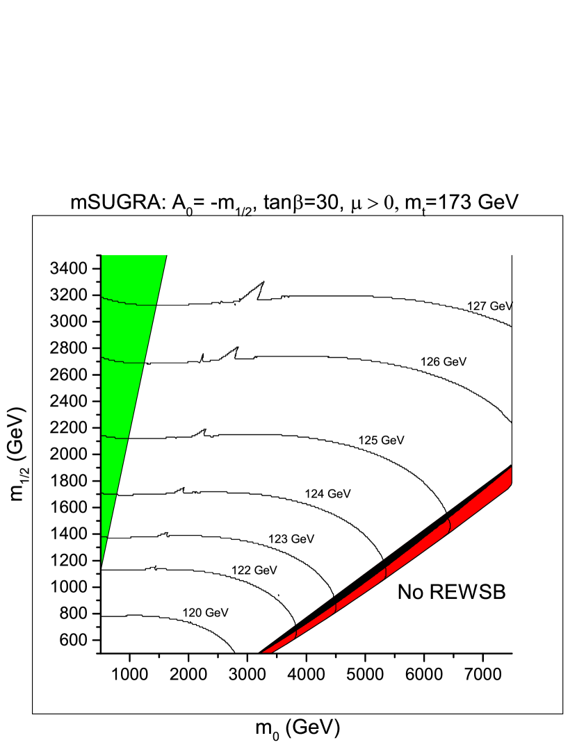
Figure 1: The mSUGRA $m_{1/2}\ vs.\ m_{0}$ plane with $A_{0}=-m_{1/2}$, $\mu>0$, tan$\beta=30$, and $m_{t}=173$ GeV. The region shaded in black indicates a relic density $0.105\lesssim\Omega_{\chi^{0}}h^{2}\lesssim 0.123$, the region shaded in red indicates $\Omega_{\chi^{0}}h^{2}\lesssim 0.123$, while the region shaded in green has a charged LSP. The black contour lines indicate the lightest CP-even Higgs mass.

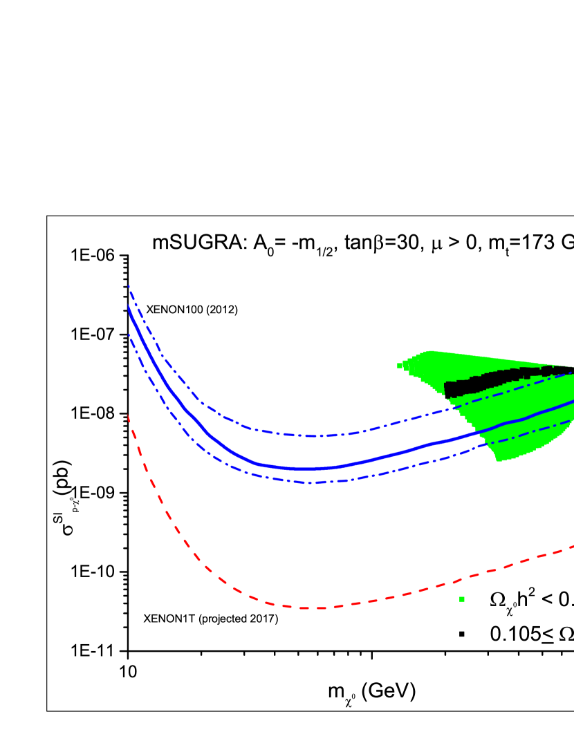
Figure 2: The spin-independent (SI) neutralino-proton direct detection cross-sections vs. neutralino mass for regions of the parameter space where $\Omega_{\chi^{0}}h^{2}\leq 0.123$. The region shaded in black indicates $0.105\lesssim\Omega_{\chi^{0}}h^{2}\lesssim 0.123$. The upper limit on the cross-section obtained from the XENON100 experiment is shown in blue with the $\pm 2\sigma$ bounds shown as dashed curves, while the red dashed curved indicates the future reach of the XENON1T experiment.

VIII Phenomenological Discussion

In the previous sections, several different forms for the supersymmetry breaking soft terms that may arise from a realistic intersecting/magnetized D-brane model were discussed. Two of these are well-known, namely the special dilaton form and the no-scale strict moduli form which arise from dilaton-dominated and K”ahler moduli dominated supersymmetry respectively. The phenomenology of both of these scenarios has been extensively explored, and neither of these two cases presently has a viable parameter space which can satisfy experimental constraints Maxin:2009pr ; Maxin:2008kp .

On the other hand, a different form for the soft terms was also explored, which appears to be a generalized form of dilaton-dominated supersymmetry breaking. In particular, it was found that if $\Theta_{1}=\Theta_{2}\equiv\Theta_{12}$ and $\Theta_{3}=\Theta_{s}\equiv\Theta_{3s}$, the universal trilinear term is always equal to the negative of the gaugino mass, $A_{0}=-m_{1/2}$. Furthermore, the universal scalar mass is given by

$$m_{1/2}=\frac{\sqrt{3}m_{3/2}}{2}(\Theta_{12}+\Theta_{3s})=\sqrt{3}m_{0}(\Theta_{12}+\Theta_{3s}).$$ (64)

From this expression, it may been observed that $m_{0}$ is always larger than the universal gaugino mass, $m_{0}>m_{1/2}$ if

$$\Theta_{12}+\Theta_{3s}<\frac{1}{\sqrt{3}}.$$ (65)

In particular, it is possible to have a scalar mass which is arbitrarily large compared to the gaugino mass such that $m_{0}>>m_{1/2}$. Generically, this may occur if either $\Theta_{12}$ or $\Theta_{3s}$ is negative.

An important question is whether or not this form for the soft terms leads to phenomenologically viable superpartner spectra. It should be noted that these soft terms correspond to one corner of the of the full mSUGRA/CMSSM parameter space. A scan of the mSUGRA/CMSSM parameter space was made in Mayes:2013qmc with the trilinear term fixed as $A_{0}=-m_{1/2}$,. A plot of this parameter space is shown in Fig. 1. As we can see from this plot, the viable parameter space consist of a strip in the $m_{0}$vs.$m_{1/2}$ plane where $m_{0}$ is several times larger than $m_{1/2}$. This, of course, corresponds to a focus point region of the hyperbolic branch of mSUGRA/CMSSM. The spectra corresponding to these regions of the parameter space feature squarks and sleptons with masses above $5$ TeV, a gluino mass in the $3-4$ TeV range, as well as neutralinos and charginos below $1$ TeV. The LSP for these spectra is of mixed bino-higgsino composition with masses in the range $300-800$ GeV. A plot of the direct dark matter detection proton-neutralino cross-sections versus neutralino mass is shown in Fig. 2. As can be seen from this plot, the direct detection cross-sections for these spectra are just in the range probed by the XENON100 experiment Aprile:2011hi ; Aprile:2012nq . In addition, the upcoming XENON1T experiment Aprile:2012zx will thoroughly cover this parameter space and either will make a discovering or rule out this parameter space, assuming R-parity conservation, leading to a stable dark matter candidate. It should be pointed out that a variation of this model exist where baryon and lepton number may be gauged, so the imposition of R-parity may not be necessary to solve the problem of rapid proton decay Maxin:2011ne .

IX Conclusion

It has been demonstrated that universal supersymmetry breaking soft terms may arise in a realistic MSSM constructed in Type II string theory with intersecting/magnetized D-branes. In particular, it has been found that these soft terms are characterized by a universal scalar mass which is always equal to one-half of the gravitino mass, and a universal trilinear term wich is always equal to the negative of the universal gaugino mass. For the simplest case where the goldstino angles for the three complex structure moduli and the dilaton are all equal, the soft terms are that of the well-known special dilaton. However, it was found that more general sets of universal soft terms with different values for the universal gaugino also exist. In particular, it was found that it is possible for the universal scalar mass to be arbitrarily large in comparison to the universal gaugino mass. Thus, for the model which has been under study, it may be natural to have scalar masses which are much larger than the gaugino mass.

While the observed mass of the Higgs is below the expected MSSM upper bound, to obtain a $125$ GeV Higgs mass requires large radiative corrections from the top/stop sector, implying heavy squarks with multi-TeV masses. Superpartner spectra with such large scalar masses may solve the hierarchy problem with low fine-tuning of the electroweak scale. The parameter space corresponding to the particular form of the soft terms $m_{0}>>m_{1/2}$ and $A_{0}=-m_{1/2}$ has been previously studied and results of this study were reviewed. Viable spectra from this region of the parameter space feature squarks and sleptons with masses above $5$ TeV, a $3-4$ TeV gluino mass, as well as light neutralinos and charginos at the TeV-scale or below. In addition, the LSP for these spectra is of mixed bino-higgsino composition with masses in the range $300-800$ GeV and a higgsino fraction of roughly $\approx 70\%$. Moreover, the spin-indepenent dark matter direct-detection proton-neutralino cross-sections are currently being probed by the XENON100 experiment and will be completely tested by the upcoming XENON1T experiment. It was shown that the soft terms corresponding to to this parameter space naturally and easily obtained from the model.

X Acknowledgments

The author would like to thank James Maxin and Dimitri Nanopoulos for helpful discussions while this manuscript was being prepared.

References

• (1)
• (2) J. R. Ellis, J. S. Hagelin, D. V. Nanopoulos and M. Srednicki, Phys. Lett. B 127, 233 (1983).
• (3) J. R. Ellis, J. S. Hagelin, D. V. Nanopoulos, K. A. Olive and M. Srednicki, Nucl. Phys. B 238, 453 (1984).
• (4) J. R. Ellis, D. V. Nanopoulos and K. Tamvakis, Phys. Lett. B 121, 123 (1983).
• (5) H. Goldberg, Phys. Rev. Lett.  50, 1419 (1983) [Erratum-ibid.  103, 099905 (2009)].
• (6) S. Dimopoulos, S. Raby and F. Wilczek, Phys. Rev. D 24, 1681 (1981).
• (7) L. E. Ibanez and G. G. Ross, Phys. Lett. B 105, 439 (1981).
• (8) G. Aad et al. [ATLAS Collaboration], Phys. Lett. B 716, 1 (2012) [arXiv:1207.7214 [hep-ex]].
• (9) S. Chatrchyan et al. [CMS Collaboration], Phys. Lett. B 716, 30 (2012) [arXiv:1207.7235 [hep-ex]].
• (10) M. S. Carena and H. E. Haber, Prog. Part. Nucl. Phys.  50, 63 (2003) [hep-ph/0208209].
• (11) G. Aad et al. [ATLAS Collaboration], arXiv:1208.0949 [hep-ex].
• (12) G. Aad et al. [ATLAS Collaboration], JHEP 1207, 167 (2012) [arXiv:1206.1760 [hep-ex]].
• (13) S. Chatrchyan et al. [CMS Collaboration], Phys. Rev. Lett.  109, 171803 (2012) [arXiv:1207.1898 [hep-ex]].
• (14) G. Aad et al. [ATLAS Collaboration], Phys. Lett. B 710, 67 (2012) [arXiv:1109.6572 [hep-ex]].
• (15) S. Chatrchyan et al. [CMS Collaboration], Phys. Rev. Lett.  107, 221804 (2011) [arXiv:1109.2352 [hep-ex]].
• (16) K. L. Chan, U. Chattopadhyay and P. Nath, Phys. Rev. D 58, 096004 (1998) [hep-ph/9710473].
• (17) J. L. Feng, K. T. Matchev and T. Moroi, Phys. Rev. Lett.  84, 2322 (2000) [hep-ph/9908309].
• (18) J. L. Feng, K. T. Matchev and T. Moroi, Phys. Rev. D 61, 075005 (2000) [hep-ph/9909334].
• (19) H. Baer, C. -h. Chen, F. Paige and X. Tata, Phys. Rev. D 52, 2746 (1995) [hep-ph/9503271].
• (20) H. Baer, C. -h. Chen, M. Drees, F. Paige and X. Tata, Phys. Rev. D 59, 055014 (1999) [hep-ph/9809223].
• (21) U. Chattopadhyay, A. Corsetti and P. Nath, Phys. Rev. D 68, 035005 (2003) [hep-ph/0303201].
• (22) S. Akula, M. Liu, P. Nath and G. Peim, Phys. Lett. B 709, 192 (2012) [arXiv:1111.4589 [hep-ph]].
• (23) P. Draper, J. Feng, P. Kant, S. Profumo and D. Sanford, arXiv:1304.1159 [hep-ph].
• (24) A. H. Chamseddine, R. L. Arnowitt and P. Nath, Phys. Rev. Lett.  49, 970 (1982).
• (25) N. Ohta, Prog. Theor. Phys.  70, 542 (1983).
• (26) L. J. Hall, J. D. Lykken and S. Weinberg, Phys. Rev. D 27, 2359 (1983).
• (27) H. Baer, V. Barger, P. Huang, D. Mickelson, A. Mustafayev and X. Tata, arXiv:1210.3019 [hep-ph].
• (28) P. G. Camara, L. E. Ibanez and A. M. Uranga, Nucl. Phys. B 689, 195 (2004) [hep-th/0311241].
• (29) V. E. Mayes, Int. J. Mod. Phys. A 28, 1350061 (2013) [arXiv:1302.4394 [hep-ph]].
• (30) G. Hinshaw, D. Larson, E. Komatsu, D. N. Spergel, C. L. Bennett, J. Dunkley, M. R. Nolta and M. Halpern et al., arXiv:1212.5226 [astro-ph.CO].
• (31) P. A. R. Ade et al. [Planck Collaboration], arXiv:1303.5076 [astro-ph.CO].
• (32) R. Blumenhagen, M. Cvetic, P. Langacker and G. Shiu, Ann. Rev. Nucl. Part. Sci.  55, 71 (2005) [arXiv:hep-th/0502005].
• (33) R. Blumenhagen, B. Kors, D. Lust and S. Stieberger, Phys. Rept.  445, 1 (2007) [arXiv:hep-th/0610327].
• (34) M. Cvetič, G. Shiu and A. M. Uranga, Phys. Rev. Lett. 87, 201801 (2001); Nucl. Phys. B 615, 3 (2001).
• (35) C. M. Chen, T. Li, V. E. Mayes and D. V. Nanopoulos, Phys. Lett.  B 665, 267 (2008) [arXiv:hep-th/0703280].
• (36) C. M. Chen, T. Li, V. E. Mayes and D. V. Nanopoulos, Phys. Rev.  D 77, 125023 (2008) [arXiv:0711.0396 [hep-ph]].
• (37) M. Cvetic, T. Li and T. Liu, Nucl. Phys.  B 698, 163 (2004) [arXiv:hep-th/0403061].
• (38) C. M. Chen, T. Li and D. V. Nanopoulos, Nucl. Phys.  B 740, 79 (2006) [arXiv:hep-th/0601064].
• (39) R. Blumenhagen, B. Körs, D. Lüst and T. Ott, Nucl. Phys.  B 616, 3 (2001) [arXiv:hep-th/0107138].
• (40) D. Cremades, L. E. Ibáñez and F. Marchesano, JHEP 0207, 009 (2002) [arXiv:hep-th/0201205].
• (41) G. Shiu and S. H. H. Tye, Phys. Rev.  D 58, 106007 (1998) [arXiv:hep-th/9805157].
• (42) M. Cvetič, P. Langacker and G. Shiu, Phys. Rev. D 66, 066004 (2002); Nucl. Phys. B 642, 139 (2002).
• (43) D. Lüst and S. Stieberger, [arXiv:hep-th/0302221].
• (44) I. Antoniadis, E. Kiritsis and T. N. Tomaras, Phys. Lett.  B 486, 186 (2000) [arXiv:hep-ph/0004214]; R. Blumenhagen, D. Lust and S. Stieberger, JHEP 0307, 036 (2003) [arXiv:hep-th/0305146].
• (45) D. Cremades, L. E. Ibáñez and F. Marchesano, JHEP 0307, 038 (2003) [arXiv:hep-th/0302105].
• (46) M. Cvetič and I. Papadimitriou, Phys. Rev.  D 68, 046001 (2003) [Erratum-ibid.  D 70, 029903 (2004)] [arXiv:hep-th/0303083].
• (47) B. Körs and P. Nath, Nucl. Phys.  B 681, 77 (2004) [arXiv:hep-th/0309167].
• (48) D. Lüst, P. Mayr, R. Richter and S. Stieberger, Nucl. Phys.  B 696, 205 (2004); A. Font and L. E. Ibanez, JHEP 0503, 040 (2005).
• (49) J. F. G. Cascales and A. M. Uranga, JHEP 0305, 011 (2003).
• (50) F. Marchesano and G. Shiu, Phys. Rev. D 71, 011701 (2005); JHEP 0411, 041 (2004).
• (51) M. Cvetič and T. Liu, Phys. Lett. B 610, 122 (2005).
• (52) M. Cvetič, T. Li and T. Liu, Phys. Rev. D 71, 106008 (2005).
• (53) J. Kumar and J. D. Wells, JHEP 0509, 067 (2005).
• (54) C.-M. Chen, V. E. Mayes and D. V. Nanopoulos, Phys. Lett.  B 633, 618 (2006).
• (55) Y. Kawamura, T. Kobayashi and T. Komatsu, Phys. Lett.  B 400, 284 (1997) [arXiv:hep-ph/9609462].
• (56) G. L. Kane, P. Kumar, J. D. Lykken and T. T. Wang, Phys. Rev.  D 71, 115017 (2005) [arXiv:hep-ph/0411125].
• (57) R. Blumenhagen, D. Lust and S. Stieberger, JHEP 0307, 036 (2003) [arXiv:hep-th/0305146].
• (58) J. A. Maxin, V. E. Mayes and D. V. Nanopoulos, Phys. Rev. D 81, 015008 (2010) [arXiv:0908.0915 [hep-ph]].
• (59) J. A. Maxin, V. E. Mayes and D. V. Nanopoulos, Phys. Rev. D 79, 123528 (2009) [arXiv:0903.4905 [hep-ph]].
• (60) J. A. Maxin, V. E. Mayes and D. V. Nanopoulos, Phys. Lett.  B 690, 501 (2010) [arXiv:0911.2806 [hep-ph]].
• (61) J. A. Maxin, V. E. Mayes and D. V. Nanopoulos, Phys. Rev.  D 79, 066010 (2009) [arXiv:0809.3200 [hep-ph]].
• (62) E. Aprile et al. [XENON100 Collaboration], Phys. Rev. Lett.  107, 131302 (2011) [arXiv:1104.2549 [astro-ph.CO]].
• (63) E. Aprile et al. [XENON100 Collaboration], Phys. Rev. Lett.  109, 181301 (2012) [arXiv:1207.5988 [astro-ph.CO]].
• (64) E. Aprile [XENON1T Collaboration], arXiv:1206.6288 [astro-ph.IM].
• (65) J. A. Maxin, V. E. Mayes and D. V. Nanopoulos, Phys. Rev. D 84, 106009 (2011) [arXiv:1108.0887 [hep-ph]].