Even-parity spin-triplet pairing for orbitally degenerate correlated electrons by purely repulsive interactions

Abstract

We demonstrate the stability of a spin-triplet paired s-wave (with an admixture of extended s-wave) state for the case of purely repulsive interactions in a degenerate two-band Hubbard model. We further show that near half-filling the considered kind of superconductivity can coexist with antiferromagnetism. The calculations have been carried out with the use of the so-called statistically consistent Gutzwiller approximation for the case of a square lattice. The absence of a stable paired state when analyzed in the Hartree-Fock-BCS approximation allows us to claim that the electron correlations in conjunction with the Hund’s rule exchange play the crucial role in stabilizing the spin-triplet superconducting state. A sizable hybridization of the bands suppresses the paired state.

Introduction.—Spin-triplet superconductivity was postulated to occur in Sr₂RuO₄Mackenzie2003 ^,Rice1994 , in uranium compoundsSaxena2000 ^-Tateiwa2001 , and in iron pnictidesDai2008 ^,Lee2008 . All these multi-band systems have moderately (Sr₂RuO₄ and the pnictides) or strongly correlated (URhGe, UPt₃) electrons, $d$ and $f$, respectively. Earlier, the spin-triplet pairing has been used successfully to describe the superfluidity of liquid ³He Anderson1973 ^,Anderson1978 and that of the neutron-star crust Pines1965 . In the last two cases of fermionic systems, which are considered as paramagnets with an enhanced susceptibility, a single-component (a single-band) Landau Fermi-liquid picture was taken as a starting point and the pairing of the odd parity (p-wave) was due to the exchange of a paramagnon. Such an approach is limited to weak correlations and was also applied to weakly ferromagnetic superconducting systemsFay1980 and to Sr₂RuO₄Mazin1997 .

In the correlated and orbitally degenerate systems the intraatomic ferromagnetic (Hund’s rule) exchange interaction of magnitude $J\sim 0.1$eV, appears naturally in the extended Hubbard model and is essential for the description of ferromagnetism, for moderately and strongly correlated electrons. On the other hand, its significance in the spin-triplet pairing has been emphasized in generalSpalek2001 ^-Puetter2012 , as well as for both the pnictides Dai2008 and Sr₂RuO₄Takimoto2000 ^-Koikegami . In most cases, the Hund’s rule and other local Coulomb interactions are either treated in the Hartree-Fock approximationZegrodnik2012 and/or semi-phenomenological negative-$U$ intersite attractionAnnett2003 is introduced. A number of experimental results can be successfully interpreted in this manner, often assuming pairing with odd angular momentum, though the situation in this respect is not yet completely clear. In effect, it is very important to scrutinize a global stability of the spin-triplet phase against an onset of either magnetism or the coexistent states within this canonical model of correlated electrons while treating both the magnetism and the pairing in real space on equal footing.

We have recently analyzed a microscopic model with the Hund’s-rule induced spin-triplet pairing, in both the Hartree-FockZegrodnik2012 and the Gutzwiller approximationZegrodnik2013 . In the Hartree-Fock-BCS limit, the paired states (often coexisting with magnetism) appear only in the limit $U^{\prime}-J=U-3J<0$, where $U^{\prime}$ is the intraatomic interorbital magnitude of the Coulomb repulsion. This limit can be called as that with attractive interactions. In the correlated Gutzwiller state and under the same conditions, superconductivity, both pure and coexistent with antiferromagnetism, is also stable Zegrodnik2013 . The stability of superconducting phases comes not as a surprise in this parameter regime, since it resembles a single band model with negative U. In the course of this study, however, it became apparent to us that the spin-triplet paired state can also become stable in the much more realistic regime of purely repulsive interactions $U^{\prime}-J>0$, a typical situation for the correlated $3d$ and $4d$ electrons. The purpose of this paper is to show that the s-wave (with a small admixture of an extended s-wave) solution, i.e., with even parity, is stable and therefore should be considered in the analysis of the spin-triplet superconductivity in the orbitally degenerate and correlated systems. We would like to underline that this is a generic microscopic approach in which the electronic correlations play a decisive role in stabilizing the spin-triplet even-parity state. Namely, the superconductivity induced by such pairing mechanism does not appear at all in the Hartree-Fock-BCS type of approach.

Model.—The starting Hamiltonian has the form of the extended Hubbard model, i.e.,

$$\begin{split}\hat{H}&=\sum_{ij(i\neq j)ll^{\prime}\sigma}t^{ll^{\prime}}_{ij}\hat{c}_{il\sigma}^{{\dagger}}\hat{c}_{jl^{\prime}\sigma}+U^{\prime}\sum_{i}\hat{n}_{i1}\hat{n}_{i2}\\ &+U\sum_{il}\hat{n}_{il\uparrow}\hat{n}_{il\downarrow}-J\sum_{ill^{\prime}(l\neq l^{\prime})}\bigg{(}\mathbf{\hat{S}}_{il}\cdotp\mathbf{\hat{S}}_{il^{\prime}}+\frac{1}{4}\hat{n}_{il}\hat{n}_{il^{\prime}}\bigg{)}\;,\end{split}$$ (1)

where $l=1,2$ labels the orbitals. The first term includes intraband ($l=l^{\prime}$) and interband (hybridization, $l\neq l^{\prime}$) hopping terms, the second and third represent the interorbital and intraorbital Coulomb repulsion, whereas the last represents the full form of the Hund’s rule exchange interaction. The Hamiltonian (1) can be rewritten in a alternative form using the real-space representation for the pairing parts

$$\begin{split}\hat{H}&=\sum_{ij(i\neq j)ll^{\prime}\sigma}t^{ll^{\prime}}_{ij}\hat{c}_{il\sigma}^{{\dagger}}\hat{c}_{jl^{\prime}\sigma}+U\sum_{il}\hat{n}_{il\uparrow}\hat{n}_{il\downarrow}\\ &+(U^{\prime}+J)\sum_{i}\hat{B}_{i}^{\dagger}\hat{B}_{i}+(U^{\prime}-J)\sum_{im}\hat{A}^{\dagger}_{im}\hat{A}_{im}\;,\end{split}$$ (2)

where the spin-triplet $\hat{A}_{im}$ and spin-singlet $\hat{B}_{i}$ pairing operators are defined as follows

$$\hat{A}^{\dagger}_{i,m}\equiv\left\{\begin{array}[]{cl}\hat{c}^{\dagger}_{i1\uparrow}\hat{c}^{\dagger}_{i2\uparrow}&m=1\;,\\ \hat{c}^{\dagger}_{i1\downarrow}\hat{c}^{\dagger}_{i2\downarrow}&m=-1\;,\\ \frac{1}{\sqrt{2}}(\hat{c}^{\dagger}_{i1\uparrow}\hat{c}^{\dagger}_{i2\downarrow}+\hat{c}^{\dagger}_{i1\downarrow}\hat{c}^{\dagger}_{i2\uparrow})&m=0\;,\\ \end{array}\right.$$ (3)

$$\hat{B}^{\dagger}_{i}\equiv\frac{1}{\sqrt{2}}(\hat{c}^{\dagger}_{i1\uparrow}\hat{c}^{\dagger}_{i2\downarrow}-\hat{c}^{\dagger}_{i1\downarrow}\hat{c}^{\dagger}_{i2\uparrow})\;.$$ (4)

As one can see, for $U^{\prime}>J$ the interaction energy that corresponds to the creation of a single pair in either spin-triplet or spin-singlet states on a atomic site, is positive. For an orbitally degenerate case, where the standard hierarchy of couplings is $U>U^{\prime}>J$, the interorbital local spin-triplet type of pairing, if any, may be favored over the singlet one. The factor favoring the triplet over the singlet pairing is the Hund’s rule exchange, but as we show, the electronic correlations are equally important to stabilize the paired state globally.

Method.—As said above, electronic correlations turn out to be crucial in this system. To include them in our study we use the modified Gutzwiller approximation. In this method, one assumes that the correlated state $|\Psi_{G}\rangle$ of the system can be expressed in the following manner

$$|\Psi_{G}\rangle=\hat{P}_{G}|\Psi_{0}\rangle\;,$$ (5)

where $|\Psi_{0}\rangle$ is the normalized non-correlated state to be defined below, whereas $\hat{P}_{G}$ is the Gutzwiller correlator, which we have selected in the form

$$\hat{P}_{G}=\prod_{i}\hat{P}_{G|i}\equiv\prod_{i}\sum_{I,I^{\prime}}\lambda_{I,I^{\prime}}|I\rangle_{ii}\langle I^{\prime}|\;.$$ (6)

Here, $\{|I\rangle\}$ is a basis of the local (atomic) Hilbert space (16 states) and $\lambda_{I,I^{\prime}}$ are variational parameters, which we assume to be real. In the subsequent discussion, we write the expectation values with respect to $|\Psi_{0}\rangle$ as $\langle\hat{O}\rangle_{0}\equiv\langle\Psi_{0}|\hat{O}|\Psi_{0}\rangle$, while the expectation values with respect to $|\Psi_{G}\rangle$ will be denoted by

$$\langle\hat{O}\rangle_{G}\equiv\frac{\langle\Psi_{G}|\hat{O}|\Psi_{G}\rangle}{\langle\Psi_{G}|\Psi_{G}\rangle}=\frac{\langle\Psi_{0}|\hat{P}_{G}\hat{O}\hat{P}_{G}|\Psi_{0}\rangle}{\langle\Psi_{0}|\hat{P}_{G}^{2}|\Psi_{0}\rangle}\;.$$ (7)

We focus on the pure superconducting phase of type A for which $\langle\hat{A}_{i,1}\rangle_{G}=\langle\hat{A}_{i,-1}\rangle_{G}\neq 0$ and $\langle\hat{A}_{i,0}\rangle_{G}\equiv 0$. This is because one would expect that the equal spin state (ESP) is favored by the local ferromagnetic exchange. Note that the expectation values in the correlated state, $|\Psi_{G}\rangle$ of the respective pairing operators are nonzero only if the corresponding expectation values in the noncorrelated state $|\Psi_{0}\rangle$ are also nonzero. For simplicity, we assume that $t^{11}=t^{22}\equiv t$ and $t^{12}=t^{21}\equiv t^{\prime}$ for the nearest neighbors. The expectation value of the grand Hamiltonian $\hat{K}=\hat{H}-\mu\hat{N}$ in the correlated state has been derived in the limit of infinite dimensions by a diagrammatic approachBunemann2005 and has the form

$$\begin{split}\langle\hat{K}\rangle_{G}&=\sum_{ijl\sigma}Q\;t_{ij}\langle\hat{c}^{\dagger}_{il\sigma}\hat{c}_{jl\sigma}\rangle_{0}+\sum_{ijll^{\prime}\sigma}Q\;t_{ij}^{\prime}\langle\hat{c}^{\dagger}_{il\sigma}\hat{c}_{jl^{\prime}\sigma}\rangle_{0}\\ &+\sum_{ij\sigma}\tilde{Q}\;t_{ij}(\langle\hat{c}^{\dagger}_{i1\sigma}\hat{c}^{\dagger}_{j2\sigma}\rangle_{0}+\langle\hat{c}_{j2\sigma}\hat{c}_{i1\sigma}\rangle_{0})\\ &+L\sum_{I,I^{\prime}}\bar{E}_{I,I^{\prime}}\langle\hat{m}_{I,I^{\prime}}\rangle_{0}-\mu\sum_{il\sigma}q^{s}_{l\sigma}\langle\hat{n}_{il\sigma}\rangle_{0}\;,\\ \end{split}$$ (8)

where $Q$ and $\tilde{Q}$ are the renormalization factors, L is the number of atomic sites, $\mu$ refers to the chemical potential, $q_{l\sigma}^{s}=\langle\hat{n}_{il\sigma}\rangle_{G}/\langle\hat{n}_{il\sigma}\rangle_{0}$, and $\hat{m}_{I,I^{\prime}}\equiv|I\rangle\langle I^{\prime}|$. The factors $Q$ and $\tilde{Q}$, as well as $\bar{E}_{I,I^{\prime}}$, can be expressed with the use of the variational parameters $\lambda_{I,I^{\prime}}$, the local single particle density matrix elements $\langle\hat{c}^{\alpha}_{il\sigma}\hat{c}^{\alpha^{\prime}}_{il^{\prime}\sigma^{\prime}}\rangle_{0}$, and the matrix elements of the atomic part of (1) represented in the local basis, $\langle I|\hat{H}^{at}|I^{\prime}\rangle$. Here $\hat{c}^{\alpha}_{il\sigma}$ are either creation or anihilation operators. The expression for $\langle\hat{K}\rangle_{G}$ can be rewritten as the expectation value of the effective single-particle Hamiltonian $\hat{K}_{GA}$, evaluated with respect to $|\Psi_{0}\rangle$, i.e.,

$$\begin{split}\hat{K}_{GA}&=\sum_{ijl\sigma}Q\;t_{ij}\hat{c}^{\dagger}_{il\sigma}\hat{c}_{jl\sigma}+\sum_{ijll^{\prime}\sigma}Q\;t_{ij}^{\prime}\hat{c}^{\dagger}_{il\sigma}\hat{c}_{jl^{\prime}\sigma}\\ &+\sum_{ij\sigma}\tilde{Q}\;t_{ij}(\hat{c}^{\dagger}_{i1\sigma}\hat{c}^{\dagger}_{j2\sigma}+\hat{c}_{j2\sigma}\hat{c}_{i1\sigma})\\ &+L\sum_{I,I^{\prime}}\bar{E}_{I,I^{\prime}}\langle\hat{m}_{I,I^{\prime}}\rangle_{0}-\mu\sum_{il\sigma}q^{s}_{l\sigma}\hat{n}_{il\sigma}\;.\\ \end{split}$$ (9)

The first three terms of (9) originate from the single particle part of (2), while the fourth originates from its interaction part. It can be seen that the intraatomic part has been taken as its average, in accordance with the general philosophy of the Gutzwiller approach. Again, the $Q$ and $\tilde{Q}$ factors are the renormalization factors of the respective dynamic processes. The first two refer to the narrowing of the quasiparticle bands, whereas the $\tilde{Q}$ parameter corresponds to the intersite pairing amplitude. It should be emphasized that in our initial Hamiltonian (1) there are no intersite interaction terms and so the intersite pairing that is present in (9) is due to correlations (a non-BCS factor). Also, the factor $\tilde{Q}$ is nonzero only when the local expectation values $\langle\hat{A}_{i,\pm 1}\rangle_{G}$ (and the corresponding $\langle\hat{A}_{i,\pm 1}\rangle_{0}$) are also nonzero. As a result, the intersite pairing appears concomitantly with the intrasite one.

In the statistically consistent Gutzwiller approach (SGA)Jedrak2010 ^,Kaczmarczyk2011 the mean fields are treated as variational parameters, with respect to which the free energy of the system is minimized. Hence, in order to assure that the self-consistent and the variational procedures yield the same results, additional constraints have to be introduced with the help of the Lagrange-multiplier method. This leads to supplementary terms in the effective Hamiltonian so that now it takes the form

$$\begin{split}\hat{K}_{\lambda}&=\hat{K}_{GA}-\lambda_{n}\big{(}\sum_{il\sigma}q^{s}_{l\sigma}\hat{n}_{il\sigma}-L\langle\hat{n}\rangle_{G}\big{)}\\ &-\sum_{m=\pm 1}\big{[}\lambda_{m}\big{(}\sum_{i}\hat{A}_{im}-L\langle\hat{A}_{im}\rangle_{0}\big{)}+H.C.\big{]}\;,\\ \end{split}$$ (10)

where the Lagrange multipliers $\lambda_{m}$ and $\lambda_{n}$ are introduced to assure that the averages $\langle\hat{A}_{im}\rangle$ and $\langle\hat{n}\rangle$ calculated either from the corresponding self-consistent equations or variationally, coincide with each other. One should also note that it is natural to fix $\langle\hat{n}\rangle_{G}$ instead of $\langle\hat{n}\rangle_{0}$ during the minimization procedure. This is the reason why we put the term $-\mu\hat{N}$ already at the beginning of out derivation. The values of the mean fields, the variational parameters, the and the Lagrange multipliers, are all found by minimizing the free energy functional $\hat{F}_{\lambda}$ that is derived with the help of the effective Hamiltonian $\hat{K}_{\lambda}$ in a standard statistical-mechanical manner. For the considered two-band model there can be up to 256 variational parameters $\lambda_{I,I^{\prime}}$. Fortunately, for symmetry reasons, one can reduce their number significantly. It should also be noted that not all of the parameters are independent, as certain constraints have to be obeyed Zegrodnik2013 ^,Bunemann2005 . In effect, we have to minimize only 16 variables in this pure superconducting state of type A.

From Eqs.(9) and (10) it can be seen that the Lagrange multipliers $\lambda_{m}$ have an interpretation of the intrasite gap parameters, while the symmetry of the intersite gap parameter is fully determined by the bare band dispersion relation. By assuming the dispersion relation for a square lattice with nonzero hopping $t$ between nearest neighbors only

$$\epsilon_{\mathbf{k}}=-2t(\cos k_{x}+\cos k_{y})\;,$$ (11)

one obtains the following form of the gap parameter

$$\Delta_{\mathbf{k}}=\Delta^{(0)}+\Delta^{(1)}(\cos{k_{x}}+\cos{k_{y}})\;,$$ (12)

where $\Delta^{(0)}\equiv\lambda_{1}=\lambda_{-1}$ (as we are considering an ESP state) while $\Delta^{(1)}\equiv 2\tilde{Q}t$ is the intersite pairing amplitude. In this manner, we have obtained a mixture of the s-wave and the extended s-wave pairing symmetry.

In order to check if the stable spin-triplet paired phases can indeed appear in the repulsive-interaction regime, we have performed first the calculations taking into account only the intrasite pairing for the following selection of phases: type A superconducting (A), pure ferromagnetic (FM), paramagnetic (NS), superconducting coexisting with antiferromagnetism (SC+AF), and pure antiferromagnetic (AF). The antiferromagnetic ordering considered by us has a simple two-sublattice form. We have also considered the so-called A1 superconducting phase ($\langle\hat{A}_{1}\rangle_{G}\neq 0$ and $\langle\hat{A}_{-1}\rangle_{G}=\langle\hat{A}_{0}\rangle_{G}\equiv 0$) coexisting with ferromagnetism. However, this phase turned out not to be stable for the whole range of model parameters examined. Therefore, it is not included in the subsequent discussion. Detailed information concerning the above phases can be found in Zegrodnik2013 , where we have analyzed the intrasite paired states in the regime of attractive interaction, i.e., for $U^{\prime}-J<0$.

Results.—The calculations have been performed assuming that the hybridization matrix element has the form $\epsilon_{12\mathbf{k}}\equiv\beta_{h}\epsilon_{\mathbf{k}}$, where $\beta_{h}\in[0,1]$, specifies the interband hybridization strength. The interorbital Coulomb repulsion constant $U^{\prime}$ was set to $U^{\prime}=U-2J$. All the energies have been normalized to the bare band-width, $W=8|t|$, and the presented results were obtained for $k_{B}T/W=10^{-4}$ emulating the $T=0$ state.

In Fig. 1 we show that the superconducting phases, both pure and coexisting with antiferromagnetism, are stable for purely repulsive interactions regime ($U^{\prime}-J>0$). With the increasing Coulomb repulsion $U$, the regions of stability of the paired phases are becoming narrower. Note that the Hartree-Fock calculations lead only to the stability of magnetically ordered phases in this regime. The appearance of the paired states is therefore a genuine many-particle effect which is caused by the electronic correlations and taken into account in the SGA method.

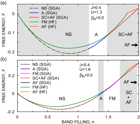
Figure 1: (Color online) Ground-state energy of stable phases as a function of the band filling for the case when only the intrasite pairing is included (i.e., for $\Delta^{(1)}\equiv 0$). For comparison, plots obtained in the H-F approximation are also shown. The shaded regions mark the stability of corresponding phases according to the SGA method. Pure AF state is stable for $n=2$ (marked by arrow).

Next, we discuss the superconducting A phase with inclusion of the intersite part of the pairing. In Fig. 2 we plot the superconducting gap components as a function of the effective pairing constant $J_{\mathrm{eff}}\equiv U^{\prime}-J$. As the value of the $J_{\mathrm{eff}}$ parameter changes sign to positive, the intra-site interaction corresponding to the spin-triplet-pair creation on a single atomic site changes from attractive to repulsive. As one could expect, according to the Hartree-Fock-BCS results, the intrasite gap parameter vanishes before $J_{\mathrm{eff}}$ reaches zero and the intersite pairing does not appear. The situation is different in the SGA. Namely, the paired solution survives for $J_{\mathrm{eff}}>0$ and the pairing has both the intra- and the inter-site components. However, the $\Delta^{(1)}$ parameter is an order of magnitude smaller than $\Delta^{(0)}$. The phase A has a lower value of energy than the normal phase for the whole range of $J_{\mathrm{eff}}$ presented in Fig. 2. Exemplary values of the order parameters, the renormalization factors, and the free energy for $T\rightarrow 0$, are all listed in Table 1.

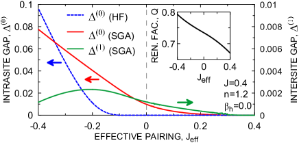
Figure 2: (Color online) The intrasite (left scale) and the intersite (right scale) gap components as a functionof the effective coupling constant $J_{\mbox{eff}}=U^{\prime}-J$. For comparison, we provide also the results obtained in the Hartree-Fock approximation. Additionally, the band renormalization factor is shown in the inset. Note that $\Delta^{(1)}=\tilde{Q}/4$.

Table 1: Representative values of the gap parameters, the renormalization factors and the free energies for $J=0.4$, $n=1.2$ and $\beta_{h}=0.0$, for three different values of the effective pairing constant, $J_{\mbox{eff}}$. For comparison, we have provided the values of the renormalization factor and the free energy for the superconducting phase of type A and the normal phase, NS. The subscripts refer to these two phases. The numerical accuracy is better that the last digit specified.

$J_{\mbox{eff}}$	$\Delta^{(0)}$	$\Delta^{(1)}$	$Q_{A}$	$Q_{NS}$	$F_{A}$	$F_{NS}$
$-0.1$	0.02325	0.00191	0.74669	0.74401	-0.255481	-0.255067
$0.1$	0.00357	0.00073	0.72164	0.72157	-0.179725	-0.179705
$0.15$	0.00200	0.00054	0.71454	0.71453	-0.161874	-0.161867

In Fig. 3a we plot the $J$ dependences of the gap parameters for $J_{\mbox{\small{eff}}}=0.1$. For larger values of $J$ the difference in magnitude between the intra- and the inter-site contributions to the pairing is not that large. The influence of the hybridization on the considered type of superconductivity is shown in Fig. 3b. The superconducting gaps are not affected by the increase of the $\beta_{h}$ parameter up to the critical value $\beta_{h}^{C}\approx 0.0379$ at which both of them suddenly drop to zero. Therefore, a sizable hybridization is detrimental to the spin-triplet pairing and the effect is strong. It means that this type of pairing suppresses the energy gain due the interorbital hopping and hence is possible only for weakly hybridized systems, where the condensation energy is dominant, $2(\Delta^{(0)})^{2}/J\gtrsim\beta_{h}/8$.

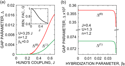
Figure 3: (Color online) Intrasite ($\Delta^{(0)}$) and intersite ($\Delta^{(1)}$) gap parameters as a function of the Hund’s exchange integral (a) and the hybridization parameter (b). In the inset of (a) the $J$ dependence of the band narrowing factor is shown.

Conclusions.—By using the SGA approach, we have shown that the intrasite spin-triplet paired states, both pure (A type) and coexistent with antiferromagnetism (SC+AF phase) can become stable in the orbitally degenerate Hubbard model, in the limit of purely repulsive interactions ($U^{\prime}-J>0$). The coexistent SC+AF phase is possible for the systems close to the half filling (the case of pnictides), whereas the pure A phase appears when $n\approx 1.2$ for doubly or when $n\approx 1.8$ for triply degenerate band which corresponds roughly to the case of Sr₂RuO₄ in the hole language. We have also analyzed the intersite pairing appearance for the considered regime of microscopic parameters. One can say that both the Hund’s rule and the correlations induced change of band energy contribute to the spin-triplet pairing mechanism; they correspond to the BCS (potential energy gain) and the non-BCS (kinetic energy gain) factors stabilizing the paired state. The intersite (extended s-wave) part of the pairing is related to the intrasite (s-wave) one. This can be seen from Figs. 2 and 3a, where $\Delta^{(0)}$ and $\Delta^{(1)}$ reach zero for the same values of model parameters. The hybridization is detrimental to the superconducting A-phase stability when the spin-triplet pairing condensation energy becomes smaller than the Pauli-principle-allowed kinetic energy gain. We believe that the combined Hund’s-rule and correlation-induced pairing presented here in the canonical model for the description of itinerant magnetism opens up new possibilities to study the spin-triplet superconductivity and its coexistence with magnetic ordering in realistic multi-band systems. Within this approach the spin-fluctuation contribution is of higher order.

M.Z. has been partly supported by the EU Human Capital Operation Program, Polish Project No. POKL.04.0101-00-434/08-00. This work has been partly supported by the Foundation for Polish Science (FNP) within project TEAM and partly by the National Science Center (NCN), through scheme MAESTRO, Grant No. DEC-2012/04/A/ST3/00342. We are also grateful to Karol I. Wysokiński for helpful discussions.

References

- (1) A. P. Mackenzie and Y. Maeno, Rev. Mod. Phys. 75, 657 (2003).
- (2) T. M. Rice and M. Sigrist, J. Phys.: Condens Matter 7, L643 (1994).
- (3) S. S. Saxena, P. Agarwal, K. Ahilan, F. M. Grosche, R. K. W. Haselwimmer, M. J. Steiner, E. Pugh, I. R. Walker, S. R. Julian, P. Monthoux, G. G. Lonzarich, A. Huxley, I. Sheikin, D. Braithwaite and J. Flouquet, Nature 406, 587 (2000).
- (4) A. Huxley, I. Sheikin, E. Ressouche, N. Kemovanois, D. Braithwaite, R. Calemczuk, J. Flouquet, Phys. Rev. B 63, 144519 (2001).
- (5) N. Tateiwa, T. C. Kobayashi, K. Hanazono, K. Amaya, Y. Haga, R. Settai and Y. Onuki, J. Phys.: Condens. Matter 13, 117 (2001).
- (6) X. Dai, Z. Fang, Y. Zhou, and F-C. Zhang, Phys. Rev. Lett 101, 057008 (2008).
- (7) P. A. Lee and X-G. Wen, Phys. Rev. B 78, 144517 (2008).
- (8) P. W. Anderson and W. F. Brinkman, Phys. Rev. Lett. 30, 1108 (1973).
- (9) P. W. Anderson and W. F. Brinkman in Physics of Liquid and Solid Helium, edited by K. H. Bennemann, and J. B. Ketterson (J. Wiley & Sons, New York, 1978) Part II, pp. 177-286.
- (10) D. Pines and A. Alpar, Nature 316, 27 (1985).
- (11) D. Fay and J. Appel, Phys. Rev. B 22, 3173 (1980).
- (12) I. I. Mazin and D. I. Singh, Phys. Rev. Lett. 79, 733 (1997).
- (13) J. Spałek, Phys. Rev. B 63, 104513 (2001).
- (14) A. Klejnberg and J. Spałek, J. Phys. C: Condens. Matter 11, 6553 (1999).
- (15) J. E. Han, Phys. Rev. B 70, 054513 (2004).
- (16) K. Sano and Y. Ono, J. Phys. Soc. Jpn 72, 1847 (2003).
- (17) C. M. Puetter and H-Y. Kee, Eur. Phys. Lett. 98, 27010 (2012).
- (18) T. Takimoto, Phys. Rev. B 62, R14641 (2000).
- (19) S. Koikegami, Y. Yoshida, and T. Yanagisawa, Phys. Rev. B 67, 134517 (2003).
- (20) M. Zegrodnik and J. Spałek, Phys. Rev. B 86 014505 (2012).
-
(21)
J. F. Annett, B. L. Györffy, G. Litak, and K. I. Wysokiński, Eur. Phys. J.
B 36, 301 (2003);
J. F. Annett, B. L. Györffy, and K. I. Wysokiński, New J. Phys. 11, 055063 (2009);
K. I. Wysokiński, J. F. Annet, and B. L. Györffy, Phys. Rev. Lett. 108, 1077004 (2012). - (22) M. Zegrodnik, J. Spałek, and J. Bünemann, arxiv: 1304.4478, unpublished
- (23) J. Bünemann, F. Gebhard, T. Ohm, S. Weiser, and W. Weber in Frontiers in Magnetic Materials (Springer, Berlin 2005).
- (24) J. Jędrak and J. Spałek, Phys. Rev. B 81 073108 (2010).
- (25) J. Kaczmarczyk and J. Spałek, Phys. Rev. B 84 125140 (2011).