Tiling simply connected regions with rectangles

Abstract.

In [BNRR], it was shown that tiling of general regions with two rectangles is NP-complete, except for a few trivial special cases. In a different direction, Rémila [Rém2] showed that for simply connected regions by two rectangles, the tileability can be solved in quadratic time (in the area). We prove that there is a finite set of at most $10^{6}$ rectangles for which the tileability problem of simply connected regions is NP-complete, closing the gap between positive and negative results in the field. We also prove that counting such rectangular tilings is #P-complete, a first result of this kind.

1. Introduction

The study of finite tilings is a classical subject of interest in both theoretical and recreational literature [Gol1, GS]. In the tileability problem, a finite set of tiles ${{\mathbf{T}}}$ is fixed, and a region is an input. This problem is known to be polynomial in some cases, and NP-complete in others (see [Pak]). Over the years, the hardness results were successively simplified (in statement, not in proof), with both sets of tiles and the regions becoming more restrictive. This paper is a new step in this direction.

In [BNRR], it was shown that tiling of general regions with two bars is NP-complete, except for the case of dominoes. In a different direction, Rémila [Rém2] (building on the ideas in [KK, Thu]), showed that for simply connected regions and two rectangles, the tileability can be solved in quadratic time (in the area). The following theorem closes the gap between these polynomial and NP-complete results.

Theorem 1.1 (Main Theorem)

There exists a finite set ${{\mathbf{R}}}$ of at most $10^{6}$ rectangular tiles, such that the tileability problem of simply connected regions with ${{\mathbf{R}}}$ is NP-complete.

Our proof of the Main Theorem is split into two parts. In the first part, we use the language of Wang tiles to reduce the Cubic Monotone $1$-in-$3$ SAT problem, known to be NP-complete, to the ${{\mathbf{T}}}$-tileability of simply connected regions with Wang tiles. In the second part, we reduce Wang tileability to tileability with rectangular tiles. Both our reductions are parsimonious and are used to prove that counting the number of tilings of simply connected regions is also hard, via reduction from 2SAT.

Theorem 1.2

There exists a finite set ${{\mathbf{R}}}$ of at most $10^{6}$ rectangular tiles, such that counting the number of tilings of simply connected regions with ${{\mathbf{R}}}$ is #P-complete.

Although #P-completeness is known for tilings of general regions with right tromino and square tetromino [MR], nothing was known for tilings with rectangles. We refer to Section 7 for the history of the problem, references, and further remarks.

2. Definitions and basic results

2.1. Ordinary tiles

Consider the integer lattice $\mathbb{Z}^{2}$ as a union of closed unit squares with pairwise disjoint interiors. A region is a finite union of such unit squares such that the interior is connected. An (ordinary) tile is a finite simply connected region.

A tileset ${{\mathbf{T}}}$ is a collection of tiles. Given a region $\Gamma$ and a tileset ${{\mathbf{T}}}$, a ${{\mathbf{T}}}$-tiling of $\Gamma$ is a union of translated copies of tiles from ${{\mathbf{T}}}$ with pairwise disjoint interiors covering $\Gamma$. If a region admits a ${{\mathbf{T}}}$-tiling then it is ${{\mathbf{T}}}$-tileable. We may simply say tiling and tileable when ${{\mathbf{T}}}$ is understood. Consider the following decision problems regarding tileability:

Simply Connected Tileability
Instance:	Simply connected region $\Gamma$, finite tileset ${{\mathbf{T}}}$.
Decide:	Whether $\Gamma$ is ${{\mathbf{T}}}$-tileable?

Simply Connected ${{\mathbf{T}}}$-Tileability
Instance:	Simply connected region $\Gamma$.
Decide:	Whether $\Gamma$ is ${{\mathbf{T}}}$-tileable?

An input region can be given by the (finite) union of the squares it contain. The following is one of the early NP-completeness results [GJ].

Theorem 2.1

If both region $\Gamma$ and tileset ${{\mathbf{T}}}$ are part of the input, Simply Connected Tileability is NP-complete in the plane.

For the rest of the paper, we will focus on finding a fixed ${{\mathbf{T}}}$ such that Simply Connected ${{\mathbf{T}}}$-Tileability is NP-complete. The following result is an extension of Theorem 2.1.

Theorem 2.2

There exists a set ${{\mathbf{T}}}$ of $\hskip 0.85355pt23$ tiles, such that Simply Connected ${{\mathbf{T}}}$-Tileability is NP-complete.

The proof follows an explicit construction of Wang tiles (see below). While we do not use Theorem 2.2, it is of independent interest, and the intermediate results in its proof provide a key step towards the proof of the Main Theorem. The history behind this theorem and its potential generalizations is outlined in Subsection 7.1.

2.2. Wang tiles

The edges of an ordinary tile are the unit-length edges on the boundary. Given a set of colors and an ordinary tile $\tau$, a generalized Wang tile is an assignment of colors to the edges of $\tau$. Note that an (ordinary) Wang tile is a generalized Wang tile of a unit square. The region $\Gamma$ we are trying to tile will also have specified colors on its boundary. A region is (Wang) tileable if there is a tiling where incident edges have the same color, including on the boundary of the region (see Figure 1). If a tileset consists of (generalized) Wang tiles, tileability always mean Wang tileability.

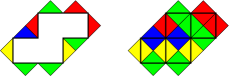
Figure 1. A colored region (left) and a Wang tiling (right). Colored edges are drawn as triangles for visibility.

2.3. Relational Wang tiles

Let us consider a more general setting. A set of relational Wang tiles is a collection ${{\mathbf{W}}}$ of squares and the following data. The vertical (respectively horizontal) Wang relation $V_{{\mathbf{W}}}(\tau,\tau^{\prime})$ (respectively $H_{{\mathbf{W}}}(\tau,\tau^{\prime})$) specify that $\tau^{\prime}\in{{\mathbf{W}}}$ is allowed to be placed immediately below (respectively to the right of) $\tau\in{{\mathbf{W}}}$. We suppress the subscripts when it can be understood from context. The boundary tiles of a region $\Gamma$ is a map from the exterior edges of $\Gamma$ to the tiles ${{\mathbf{W}}}$. By abuse of language, we define the notion of tiling in this context:  a ${{\mathbf{W}}}$-tiling of a region $\Gamma$ is a map $\pi:\Gamma\to W$ such that tiles placed next to each other satisfy the Wang relations. Whenever a tile is adjacent to an exterior edge, we check the Wang relations as if the boundary tile corresponding to the edge is on the other side of the edge.

2.4. Complexity

Throughout the paper we consider many tiling problems that are NP-complete. All these problems are trivially in NP. Indeed, given a description of a tiling, one could simply check if it is in fact a tiling. To prove NP-hardness, we reduce a known NP-complete problem to the problem in question. We refer to [GJ, Pap] for definitions and details.

We will embed Cubic Monotone $1$-in-$3$ SAT as a tiling problem. Let $X=\{x_{1},\ldots,x_{n}\}$ be a set of boolean variables. A (monotone $1$-in-$3$) clause $C$ is a set of three variables. A (cubic monotone $1$-in-$3$) expression $E$ is a finite collection $\mathcal{C}$ of monotone $1$-in-$3$ clauses, where each variable $x_{i}\in X$ occurs three times. We say such $E$ is ($1$-in-$3$) satisfiable if there is an assignment of boolean values $\{0,1\}$ to the variables $x_{i}\in X$ such that each clause in $E$ contains precisely one variable receiving $1$ (and thus two variables receiving $0$).

Cubic Monotone $1$-in-$3$ SAT
Instance:	Set $X$ of variables, cubic monotone expression $E$.
Decide:	Whether $E$ is $1$-in-$3$ satisfiable?

The following result was shown by Gonzalez in the language of exact covers:

Theorem 2.3 ([Gon])

Cubic Monotone $1$-in-$3$ SAT is NP-complete.

We will reduce Cubic Monotone $1$-in-$3$ SAT to a tiling problem Simply Connected ${{\mathbf{T}}}$-Tileability for some fixed ${{\mathbf{T}}}$.

2.5. Counting problems

Throughout the paper we consider natural counting problems corresponding to the decision problems. For example, instead of asking whether satisfying assignments exist, we ask how many satisfying assignments there are. Similarly, for tileability, we count the number of tilings. If in the proof of NP-completeness, the corresponding reductions give a bijection between the sets of solutions, we call such reduction parsimonious.

Parsimonious reductions have the additional benefit of proving counting results using the same reduction. The class #P consists of the counting problems associated with decisions problems in NP. A counting problem is #P-complete if it is in #P and every #P question can be reduced to it. Thus, if there is a parsimonious reduction from problem $Q_{1}$ to $Q_{2}$, then if $Q_{1}$ is #P-complete, then so is $Q_{2}$. We refer to [Val] (see also [Pap]) for definitions and details on #P complexity class.

One main goal is to reduce Cubic Monotone $1$-in-$3$ SAT to a tiling problem Simply Connected ${{\mathbf{T}}}$-Tileability for some fixed ${{\mathbf{T}}}$. This reduction will turn out to be parsimonious, hence the number of satisfying assignments of a given instance of the satisfiability problem can be calculated by counting the number of tilings of the transformed instance.

However, it is not known whether the associated counting problem #Cubic Monotone $1$-in-$3$ SAT is #P-complete. To get the #P-completeness result in Theorem 1.2, we will modify the reduction to use 2SAT instead, whose associated counting problem #2SAT is #P-complete.

3. Reduction lemmas

3.1. Basic reductions

In this section we consider five classes of Tileability problems. Let $\mathcal{T}$ be a collection of tiles and $\mathcal{R}$ be a collection of regions. A decision problem in $(\mathcal{T},\mathcal{R})$-Tileability consists of a fixed tileset ${{\mathbf{T}}}\subset\mathcal{T}$, receives some $\Gamma\in\mathcal{R}$ as input, and outputs whether $\Gamma$ is ${{\mathbf{T}}}$-tileable.

We say $(\mathcal{T},\mathcal{R})$-Tileability is linear time reducible to $(\mathcal{T}^{\prime},\mathcal{R}^{\prime})$-Tileability if for any finite tileset ${{\mathbf{T}}}\subset\mathcal{T}$, there exists a finite tileset ${{\mathbf{T}}}^{\prime}\subset\mathcal{T}^{\prime}$ and a reduction map $f:\mathcal{R}\to\mathcal{R}^{\prime}$ that is computable in linear time (in the complexity of $\Gamma\in\mathcal{R}$), such that $\Gamma\in\mathcal{R}$ is ${{\mathbf{T}}}$-tileable if and only if $f(\Gamma)$ is ${{\mathbf{T}}}^{\prime}$-tileable. If, moreover, that $(\mathcal{T}^{\prime},\mathcal{R}^{\prime})$-Tileability is linear time reducible to $(\mathcal{T},\mathcal{R})$-Tileability, then they are linear time equivalent. Note that the transformation of the tilesets need not be efficient nor bijective.

For instance, if $\mathcal{T}$ is the collection of all rectangular tiles and $\mathcal{R}$ consists of simply connected regions, then $(\mathcal{T},\mathcal{R})$-Tileability is a class of problems regarding tiling simply connected regions with rectangular tiles. To simplify the notation, we drop the prefix in $(\mathcal{T},\mathcal{R})$-Tileability when the sets $\mathcal{T}$ and $\mathcal{R}$ are understood.

Lemma 3.1 (Tileability Equivalence Lemma)

The following five classes of Simply Connected Tileability problems are linear time equivalent:

1. Tileability with a fixed set of rectangular tiles.

2. Tileability with a fixed set of ordinary tiles.

3. Tileability with a fixed set of generalized Wang tiles.

4. Tileability with a fixed set of ordinary Wang tiles.

5. Tileability with a fixed set of relational Wang tiles.

Moreover, the size of the tileset can be preserved in the reductions between (ii) and (iii).

Proof.

The reductions (i)$\Rightarrow$(ii)$\Leftrightarrow$(iii)$\Rightarrow$(iv)$\Rightarrow$(v) are elementary and given below. The reduction (v)$\Rightarrow$(i) is stated separately as Lemma 3.3 and proved in the next section.

We may consider a rectangular tile as an ordinary tile, which in turn is a monochromatic generalized Wang tile. Therefore the reductions (i)$\Rightarrow$(ii)$\Rightarrow$(iii) are immediate, where each reduction map is simply the identity.

(iii)$\Rightarrow$(iv). Given a set of generalized Wang tiles, color each interior edge with a new color not used anywhere else, and consider each square as a separate ordinary Wang tile (see Figure 2). These tiles are forced to reassemble themselves as the original generalized Wang tiles. The reduction map is again the identity.

(iv)$\Rightarrow$(v). It is obvious how to define the Wang relations to mimic the colored Wang tiles without increasing the number of tiles. To encode the boundary conditions, we may need to introduce less than $4\chi$ tiles, where $\chi$ is the number of colors permitted on the boundary. Indeed, to specify a color $c$ on the top boundary, we need to choose an (arbitrary) tile whose bottom color is $c$. If no such tile exists, we must add a new tile to do so. If we do not involve the new tile in any Wang relations in the other directions, then it will never be used in the actual tiling, and thus will not affect tileability. We do the same for the other three directions.

The final reduction (v)$\Rightarrow$(i) is more difficult and is the content of Lemma 3.3 and proved in a later section.

To preserve the number of tiles in (iii)$\Rightarrow$(ii), scale the generalized Wang tile and replace each colored edge by an appropriate rectilinear zig-zag curve to encode the matching rules (see Figure 3 and [Gol2]). ∎

(a)

(b)

(c)

(d)

(e)

Figure 2. From generalized Wang tiles to ordinary ones.

(a)

(b)

(c)

Figure 3. Replacing each colored edge by a zig-zag curve to get ordinary tiles.

3.2. Two main reductions

Lemma 3.2 (First Reduction Lemma)

There exists a set ${{\mathbf{T}}}$ of at most $23$ generalized Wang tiles with total area $133$ and using $9$ colors such that Simply Connected ${{\mathbf{T}}}$-Tileability is NP-complete. Moreover, this will be achieved by a parsimonious reduction from Cubic Monotone $1$-in-$3$ SAT.

Lemma 3.3 (Second Reduction Lemma)

For a set ${{\mathbf{W}}}$ of at most $k$ (ordinary) Wang tiles with $c$ (boundary) colors, there exists a set ${{\mathbf{R}}}$ of at most $8(k+4c)^{2}$ rectangular tiles with the following property. Given a simply connected colored region $\Gamma$, there is a simply connected region $\Gamma^{\prime}$ such that $\Gamma$ is ${{\mathbf{W}}}$-tileable if and only if $\Gamma^{\prime}$ is ${{\mathbf{R}}}$-tileable. Moreover, this reduction is parsimonious and can be computed in linear time.

We may transform the set of $23$ generalized Wang tiles afforded by Lemma 3.2, according to the procedure outlined in (iii)$\Rightarrow$(ii) of Lemma 3.1, in order to obtain Theorem 2.2 using $23$ ordinary tiles. Similarly, using the transformation of Lemma 3.3, we conclude the result for rectangular tiles in Theorem 1.1 (see Subsection 6.1). Theorem 1.2 can be shown by modifying the proof of Lemma 3.2 to achieve a parsimonious reduction from, say, 2SAT, whose associated counting problem is #P-complete (see Subsection 6.2).

4. Proof of the First Reduction Lemma (Lemma 3.2)

4.1. General setup

The goal of this section is to construct a set of generalized Wang tiles that could be used to solve Cubic Monotone $1$-in-$3$ SAT. Each expression will be encoded as a colored rectangular boundary. Tiles corresponding to variables and clauses will appear on the left and right sides of the region, respectively. The variable tiles will “transmit” its state ($0$ or $1$) through “wires” to the clause tiles; each clause tile will “check” if precisely one out of three signals it receives is $1$. The path of the transmissions will be regulated by placing “crossover tiles” that allow signals to crossover at specific locations. The positioning of such tiles will be enforced by using a combination of “control tiles” that follow instructions encoded on the boundary. Empty spaces will be filled by “filler tiles.”

4.2. Tileset ${{\mathbf{T}}}$

Let ${{\mathbf{T}}}$ be a tileset with the $7$ small tiles shown in Figure 4 and the $3$ big tiles in Figure 5. Some horizontal edges are colored by their labels; all unlabeled edges are colored by $0$, which is omitted in the figures for clarity, but acts as any other ordinary color.

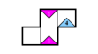
(a) $L$

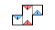
(b) $W$

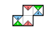
(c) $S$

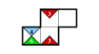
(d) $R$

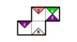
(e) $B$

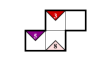
(f) $K$

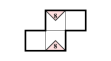
(g) $F$

Figure 4. Tiles in tileset ${{\mathbf{T}}}$.

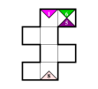
(a) $X$

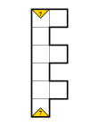
(b) $V$

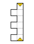
(c) $C$

Figure 5. More tiles in ${{\mathbf{T}}}$.

4.3. Tileset ${{\mathbf{T}}}^{\prime}$

Recall that the vertical edges of our tiles in ${{\mathbf{T}}}$ are all colored with $0$. Form ${{\mathbf{T}}}^{\prime}$ by recoloring the vertical edges of tiles in ${{\mathbf{T}}}$ as follows. Given each small tile $\tau\in{{\mathbf{T}}}$ in Figure 4, we introduce a variant by coloring all its vertical edges with $1$. The color of the vertical edges is called the parity of $\tau$. Include both this variant and the original in ${{\mathbf{T}}}^{\prime}$.

Given a rectangular array of these tiles, the parities are consistent across each row and are independent across the columns. Intuitively, these tiles act as wires that can transmit data (parity of the tile) horizontally across the region.

We continue defining ${{\mathbf{T}}}^{\prime}$. We add three new versions of the crossover tile $X$ as in Figure 6a. Intuitively, this allows the data transmissions to crossover. We also add a variant of the variable tile $V$, as in Figure 6b, where all the right vertical edges are colored with $1$. The parity of the variable tile corresponds to the truth value assigned to that variable. Finally, we replace the clause tile $C$ by the three shown in Figure 6c, where each tile has one out of three pairs of left vertical edges colored with $1$. Thus ${{\mathbf{T}}}^{\prime}$ consists of $23$ tiles.

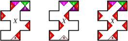
(a) $X$

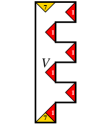
(b) $V$

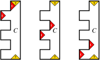
(c) $C$

Figure 6. Variations of tiles in ${{\mathbf{T}}}$.

We will place the variable tiles on the left and the clause tiles on the right. It remains to send the data from the variables to the correct clauses. We achieve this by specifying boundary colors to force crossover tiles to appear at the desired locations.

4.4. Reduction construction

Our goal is to embed the decision problem Cubic Monotone $1$-in-$3$ SAT as a tiling problem. Given a cubic monotone $1$-in-$3$ SAT expression $E$ with variables $X=\{x_{1},\ldots,x_{n}\}$ and clauses $\mathcal{C}=\{C_{1},\ldots,C_{n}\}$, consider it as a permutation $\sigma=\sigma_{E}\in S_{3n}$ in the symmetric group on $3\hskip 0.85355ptn$ letters as follows. Think of $\sigma$ as a bijection from the ordered multiset $X^{\prime}=\{x_{1},x_{1},x_{1},x_{2},\ldots,x_{n}\}$ to the ordered multiset $\mathcal{C}^{\prime}=\{C_{1},C_{1},C_{1},C_{2},\ldots,C_{n}\}$, where each variable and each clause is listed three times. For each $x_{i}\in C_{j}$, we have $\sigma(x_{i})=C_{j}$ once. Now identify each multiset with $[3n]=\{1,2,\ldots,3n\}$ to get $\sigma$ as a permutation in $S_{3n}$. Let $s_{i}=(i,i+1)$ be an adjacent transposition for $i\in[3n-1]$. Write $\sigma=s_{i_{1}}s_{i_{2}}\ldots s_{i_{d}}$ as a product of adjacent transpositions, with $d=O(n^{2})$.

Let $c_{k}$ be the color sequence $01(02)^{k-1}63$. Define a rectangular region $\Gamma=\Gamma_{E}$ as follows. The height of $\Gamma$ is $6n$ and the vertical edges are colored with $0$. The width is the length of the color sequence $7c_{i_{1}}c_{i_{2}}\ldots c_{i_{d}}07$, which is used as the top boundary. The bottom boundary is $7(08)^{t}07$ with the same length as the top boundary. The following result demonstrates the ability to place the crossover tile $X$ at arbitrary depth of a large rectangular region.

Sublemma 4.1

The region $\Gamma$ admits a unique ${{\mathbf{T}}}$-tiling.

Proof.

The left and right sides are forced to be filled with variable and clause tiles, respectively. Now consider the section in between.

For $k\geq 1$ and $\ell\geq 0$, consider a row of tiles $LW^{k}S^{\ell}R$ (meaning an $L$ tile followed by a $W$ tiles $k$ times, an $S$ tile $\ell$ times, and ending with an $R$ tile). The bottom color sequence is $01(02)^{k}(62)^{\ell}63$. One easily checks that the unique way to tile the next row is with $LW^{k-1}S^{\ell+1}R$.

If $k=0$, we get the case where we have a row $LS^{\ell}R$ with bottom color sequence $01(62)^{\ell}63$. The unique way to tile the next row is with $XB^{\ell}K$.

The section below will be filled by filler tiles $F$. Thus every section below $c_{i}$ is filled uniquely, with the crossover tile $X$ occupying rows $i$ and $i+1$ in the first column. ∎

The above proof is illustrated with two examples in the next subsection.

Corollary 4.2

The expression $E$ is satisfiable if and only if $\Gamma_{E}$ is ${{\mathbf{T}}}^{\prime}$-tileable. Moreover, the reduction is parsimonious, that is, the number of tilings of $\Gamma_{E}$ is the number of satisfying assignments for $E$.

The corollary follows immediately from the construction given above, and concludes the proof of Lemma 3.2.

4.5. Examples of the tiling construction

In Figure 7 we show how to place a crossover tile in a special case, corresponding to expression $\{(x,y,x),(x,y,y)\}$. We illustrate the crossings with a wiring diagram and then give a complete Wang tiling. In Figure 8 below we give a bigger example of the wiring diagram and the unique Wang tiling, corresponding to expression $\{(x,y,x),(x,y,z),(y,z,z)\}$.

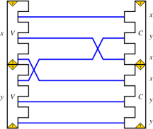
(a) Wiring diagram

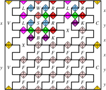
(b) Unique tiling

Figure 7. A small example of how to place crossover tiles.

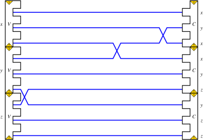
(a) Wiring diagram

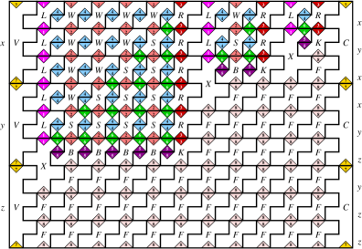
(b) Unique tiling

Figure 8. A bigger example of the unique base tiling.

5. Proof of the Second Reduction Lemma (Lemma 3.3)

5.1. Basics

In this section, we provide a further connection between Wang tiles and ordinary rectangular tiles (by making a reduction from the latter to the former). Recall that by Lemma 3.1, we can replace generalized Wang tiles with relational Wang tiles.

Without loss of generality, we may assume that the Wang relations are irreflexive, that is, there is no tile $\tau$ such that $H(\tau,\tau)$ or $V(\tau,\tau)$. Indeed, suppose ${{\mathbf{W}}}$ is a set of Wang tiles. Let ${{\mathbf{W}}}^{\prime}=\{\tau_{i}:i\in\{0,1\},\ \tau\in{{\mathbf{W}}}\}$ be a doubled set of tiles. Define its horizontal Wang relation as follows. For $\tau,\tau^{\prime}\in{{\mathbf{W}}}$ and $i,j\in\{0,1\}$, let $H_{{{\mathbf{W}}}^{\prime}}(\tau_{i},\tau^{\prime}_{j})$ if and only if $H_{{{\mathbf{W}}}}(\tau,\tau^{\prime})$ and $i\neq j$. Its vertical Wang relation is defined analogously. It is clear that the Wang relations of ${{\mathbf{W}}}^{\prime}$ are irreflexive. Moreover, a ${{\mathbf{W}}}$-tiling can be made into a ${{\mathbf{W}}}^{\prime}$-tiling by adding subscripts to the tiles in a checkerboard fashion, while the reverse can be done by ignoring the subscripts. Of course, the same transformation is done on the boundary tiles as well. Clearly this does not affect tileability nor the number of such tilings.

From now on, assume we are given a fixed set ${{\mathbf{W}}}$ of relational Wang tiles whose relations $H$ and $V$ are irreflexive. Our goal is to produce a fixed set ${{\mathbf{R}}}$ of rectangular tiles with the following property: Given any simply connected region $\Gamma$ with specified boundary tiles, we can produce (in linear time) a simply connected region $\Gamma^{\prime}$ such that $\Gamma$ is ${{\mathbf{W}}}$-tileable if and only if $\Gamma^{\prime}$ is ${{\mathbf{R}}}$-tileable. Moreover, the number of ${{\mathbf{W}}}$-tilings of $\Gamma$ will be the same as the number of ${{\mathbf{R}}}$-tilings of $\Gamma^{\prime}$.

For simplicity, we first consider the case where we are given an $r\times c$ rectangular region $\Gamma$ with specified boundary tiles.

5.2. Expansion

From this point on, we only consider tiling using rectangular tiles. Fix $M$ and $e$ to be positive integers. Given a region $\Gamma_{0}$, we obtain an $(M,e)$-expansion $\Gamma$ by scaling $\Gamma_{0}$ by a factor of $M$ and then perturb it by moving each corner vertex of the boundary curve of the region $\Gamma$, at most $e$ in each direction, such that $\Gamma$ is still a region (with rectilinear edges). Recall that a (rectangular) tile is just a simply connected region, thus the notion of $(M,e)$-expansion of a tile is defined. A tileset ${{\mathbf{T}}}$ is an $(M,e)$-expansion of a tileset ${{\mathbf{T}}}_{0}$ if each $\tau\in{{\mathbf{T}}}$ is an $(M,e)$-expansion of some $\tau_{0}\in{{\mathbf{T}}}_{0}$.

A tiling $\pi$ of a region $\Gamma$ is an $(M,e)$-expansion of a tiling $\pi_{0}$ of some region $\Gamma_{0}$ if it can be obtained by dilating by a factor of $M$, and then perturbing the tiles and the region by at most $e$ as above. Note that after scaling, each tile may grow or shrink in each dimension by at most $2e$, and can shift around from its starting point by at most $e$.

Given a tileset ${{\mathbf{T}}}_{0}$ and an $(M,e)$-expansion ${{\mathbf{T}}}$, a region $\Gamma$ respects the expansion if there is a unique region $\Gamma_{0}$ such that any ${{\mathbf{T}}}$-tiling of $\Gamma$ is an $(M,e)$-expansion of a ${{\mathbf{T}}}_{0}$-tiling of $\Gamma_{0}$.

Intuitively, we will choose $M>100e$, say, and carefully perturb only a few tiles, so that when consider tilings of regions respecting the expansion, we can essentially predict what the new tiling can be based on the original tiling.

5.3. Rectangular tiles ${{\mathbf{R}}}_{0}$ and the region $\Gamma_{0}(r,c)$

Consider the following tileset:

$${{\mathbf{R}}}_{0}=\left\{f=R(34,11),\ w=R(31,14),\ s=R(10,10),\ h=R(11,31),\ v=R(14,34)\right\},$$

where $R(a,b)$ denotes a rectangle of height $a$ and width $b$ (see Figure 9). For a rectangle $t$, write $\text{{\bf ht\hskip 0.85355pt}}t$ and $\text{{\bf wd\hskip 0.85355pt}}t$ for its height and width, respectively.

(a)

(b)

(c)

(d)

(e)

Figure 9. Rectangular tiles ${{\mathbf{R}}}_{0}$.

Now consider the region $\Gamma_{0}(r,c)$ defined as follows (see Figure 10). On each vertical side, there are $r$ protrusions of height $\text{{\bf ht\hskip 0.85355pt}}h$ and width $\text{{\bf wd\hskip 0.85355pt}}s$, separated by height $\text{{\bf ht\hskip 0.85355pt}}f$. On each horizontal side, there are $c$ cavities of width $\text{{\bf wd\hskip 0.85355pt}}v$ and height $\text{{\bf ht\hskip 0.85355pt}}s$, separated by width $\text{{\bf wd\hskip 0.85355pt}}f$.

Figure 10. Boundary region $\Gamma_{0}(2,2)$.

Sublemma 5.1

The unique ${{\mathbf{R}}}_{0}$-tiling of $\Gamma_{0}(r,c)$ consists of $r$ rows and $c$ columns of the $w$ tile.

Proof.

Fix natural numbers $a=10$ and $b=1$. The tiles introduced above can now be written as $f=R(3a+4b,a+b)$, $w=R(3a+b,a+4b)$, $s=R(a,a)$, $h=R(a+b,3a+b)$, and $v=R(a+4b,3a+4b)$.

We begin with a few definitions. A horizontal (vertical) segment of a region is called bounded if the region extends downward (to the right) on both sides of the segment. For $t\in\{v,h\}$, a pair $(t,s)$ is the configuration of placing the tile $s$ above or below $t$, aligned on the left. The orientation of the pair is positive (negative) if $s$ is placed below (above). Similarly, for $t\in\{w,f\}$, a pair $(t,s)$ is obtained by placing $s$ to the left or right of $t$, aligned on top. The orientation is positive (negative) if $s$ is placed to the right (left). A bounded segment is tiled by a tile (pair) if in all tilings, the tile (pair) is adjacent to the segment.

We will tile the region $\Gamma_{0}(r,c)$ in steps, as indicated by the numbers labeled on Figure 11. Note that since $a>b$, each bounded horizontal segment of width $\text{{\bf wd\hskip 0.85355pt}}f$ on the top border must be tiled by $f$ tiles, labeled 1. Similarly on the left, the bounded vertical segments of height $\text{{\bf ht\hskip 0.85355pt}}h$ must be tiled by $h$ tiles, labeled 2. This creates a bounded vertical segment of height $\text{{\bf ht\hskip 0.85355pt}}v+\text{{\bf ht\hskip 0.85355pt}}s$ on the top left corner; since $a>3b$, it is tiled by the pair $(v,s)$, labeled 3. Since $a>4b$, it is obvious that it needs to be positively oriented, to avoid a hole of width $\text{{\bf wd\hskip 0.85355pt}}v-\text{{\bf wd\hskip 0.85355pt}}s$ and height $\text{{\bf ht\hskip 0.85355pt}}s$, which cannot be filled.

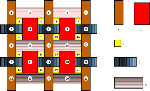
Figure 11. Unique base tiling labeled by order.

Note that since $a>3b$, this creates a new bounded horizontal segment of width $\text{{\bf wd\hskip 0.85355pt}}w+\text{{\bf wd\hskip 0.85355pt}}s$, which is tiled by the pair $(w,s)$, labeled 4. If $w$ is on the left, it will create a bounded horizontal segment of width $\text{{\bf wd\hskip 0.85355pt}}f+\text{{\bf wd\hskip 0.85355pt}}s$ to its left. Otherwise, if $w$ is on the right, several $s$ will be forced to appear on the left and still create the same bounded segment. Therefore, the $(w,s)$ pair creates the bounded segment, regardless of how it is oriented.

Since $a>3b$, this bounded horizontal segment of width $\text{{\bf wd\hskip 0.85355pt}}f+\text{{\bf wd\hskip 0.85355pt}}s$ is again tiled by an $(f,s)$ pair, labeled 5. Like the $(v,s)$ pair above, since $a>4b$, this needs to be positively oriented. This creates the bounded vertical segment of height $\text{{\bf ht\hskip 0.85355pt}}v+\text{{\bf ht\hskip 0.85355pt}}s$, tiled by a pair $(v,s)$, labeled 6, as above. In either orientation, it bounds the vertical segment of height $\text{{\bf ht\hskip 0.85355pt}}w$ above, concluding that the $(w,s)$ pair (labeled 4) we placed above needs to be positively oriented. Furthermore, this bounds the vertical segment of height $\text{{\bf ht\hskip 0.85355pt}}h+\text{{\bf ht\hskip 0.85355pt}}s$, again tiled by the pair $(h,s)$, labeled 7. As before, in either orientation, we have a bounded vertical segment of height $\text{{\bf ht\hskip 0.85355pt}}v+\text{{\bf ht\hskip 0.85355pt}}s$, which necessarily needs to be tiled by the positively oriented pair $(v,s)$, labeled 8. This creates a bounded horizontal segment of width $\text{{\bf wd\hskip 0.85355pt}}w+\text{{\bf wd\hskip 0.85355pt}}s$.

We continue in like manner, working our way on the anti-diagonal from top right to bottom left. Each time we place the pair $(w,s)$, forcing the adjacent pair $(h,s)$ placed in the previous stage to be positively oriented. Then we place $(f,s)$, forcing the adjacent $(v,s)$ to be positively oriented as well. This procedure repeats with $(w,s)$ and $(f,s)$ in an alternating fashion. The last $(f,s)$ will be placed in positive orientation and creates a bounded vertical segment of height $\text{{\bf ht\hskip 0.85355pt}}v+\text{{\bf ht\hskip 0.85355pt}}s$.

Similarly, we work from bottom left to top right on the next anti-diagonal. We alternate between placing $(v,s)$ and $(h,s)$ pairs, positively orienting the $(w,s)$ and $(f,s)$ pairs in the previous stage, respectively. This continues until the entire region is filled. ∎

5.4. Expansion ${{\mathbf{R}}}$ of ${{\mathbf{R}}}_{0}$

We will now define a clever set of perturbed expansion tiles that will correspond to the relational Wang tiles. Only the tiles $s$, $h$, and $v$ will have perturbations. Let ${{\mathbf{W}}}=\{\tau_{1},\ldots,\tau_{n}\}$ be the fixed set of relational Wang tiles with irreflexive horizontal and vertical Wang relations $H$ and $V$, respectively. Fix $e=5^{n}$ and $M=100e$ for the remainder of the section. Let ${{\mathbf{R}}}$ be an $(M,e)$-expansion of ${{\mathbf{R}}}_{0}$ as follows:

For $t\in\{s,h,v\}$, let $t(a,b)$ be the scaled version of $t$ with height and width increased by $a$ and $b$, respectively. Imagine that the $h$ and $v$ tiles can stretch horizontally and vertically, respectively, and the $s$ tiles can stretch in both directions. Then the $w$ tiles, having no perturbations, will only shift around a little (by at most $e$). The $f$ tiles will stay fixed, enforcing the global structure. See Figure 12. A $w$ tile will be shifted to the right and down by $5^{i}$ to represent the Wang tile $\tau_{i}$. To restrict the shifts to only those sizes, we replace $s$ with the appropriate perturbed versions. Namely, for each $i$, introduce four tiles with perturbations $s(\pm 5^{i},\pm 5^{i})$, where all four combinations of signs are included. To enforce the Wang relations, for each $\tau_{i},\tau_{j}\in{{\mathbf{W}}}$ such that $V(\tau_{i},\tau_{j})$ or $H(\tau_{i},\tau_{j})$, we introduce the perturbation $v(5^{j}-5^{i},0)$ or $h(0,5^{j}-5^{i})$, respectively. This is the set ${{\mathbf{R}}}$ we will use.

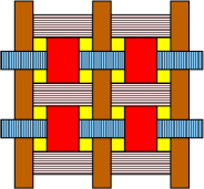
(a)

(b)

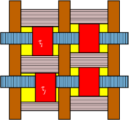
(c)

Figure 12. Shifting an expansion of the unique tiling to represent Wang tiles.

5.5. Rectangular tiling

Obtain an $(M,e)$-expansion $\Gamma(r,c)$ of $\Gamma_{0}(r,c)$ by scaling with a factor of $M$ and then perturbing it as follows. Recall that there are $r$ protrusions on each vertical side and $c$ cavities on each horizontal side. Each protrusion or cavity corresponds to a boundary tile of $\Gamma$ in a natural way. Perturb the protrusion or cavity to the right or down, respectively, by $5^{i}$ units if it corresponds to $\tau_{i}$.

Sublemma 5.2

The $(M,e)$-expansion $\Gamma(r,c)$ of $\Gamma_{0}(r,c)$ respects the expansion ${{\mathbf{R}}}$ of ${{\mathbf{R}}}_{0}$.

Proof.

Recall the argument in the proof of Sublemma 5.1. As the inequalities are all satisfied, the $f$ tiles are fixed and force the perturbations to stay local. The $w$ tiles have two degrees of freedom. They can move $\pm 5^{i}$ in each direction, as regulated by the $s$ tiles. Now note that the inequalities in the proof of Sublemma 5.1 are preserved. We leave the (easy) details to the reader. ∎

We now return to the proof of Lemma 3.3. It is clear that given a Wang ${{\mathbf{W}}}$-tiling of the rectangle $\Gamma$ with boundary, we will get an ${{\mathbf{R}}}$-tiling of $\Gamma(r,c)$. Indeed, simply take the unique tiling of $\Gamma_{0}(r,c)$ as afforded by Sublemma 5.1, scale by a factor of $M$, and then shift each $w$ tile to the right and down by $5^{i}$ if it represents $\tau_{i}$, and adjust the other tiles in the obvious way.

Conversely, if we are given an ${{\mathbf{R}}}$-tiling of $\Gamma(r,c)$, we wish to recover the ${{\mathbf{W}}}$-tiling of $\Gamma$. This is achieved using the following two sublemmas, both of which are clear when all numbers are considered in base $5$; we omit the (easy) details.

Sublemma 5.3

The equation $5^{i}-5^{j}=5^{k}+5^{\ell}$ does not admit a solution in $\mathbb{N}$.

Therefore each $w$ tile will shift to the right and down (as opposed to shifting left or up), and hence indeed represents a Wang tile $\tau_{i}$ for some $i$.

Sublemma 5.4

The equation $5^{i}-5^{j}=5^{k}-5^{\ell}$ does not admit solutions in $\mathbb{N}$ except if $i=j$ or $i=k$.

If a $w$ tile representing $\tau_{j}$ is to the right of a $w$ tile representing $\tau_{i}$, then $h(0,5^{j}-5^{i})$ must be in ${{\mathbf{R}}}$. By the sublemma above, the differences $5^{j}-5^{i}$ are all distinct (recall that the Wang relations are irreflexive, so $i=j$ does not happen), therefore we must have had $H(\tau_{i},\tau_{j})$ as part of the Wang relation. Similarly for the vertical Wang relation $V$. So by reading off the associated tile $\tau_{i}$ from the shifts of each $w$ tile, we get a Wang ${{\mathbf{W}}}$-tiling of $\Gamma$.

This completes the construction of $\Gamma_{0}(r,c)$ for the case when $\Gamma$ is a rectangle. For the general case, when $\Gamma$ is a simply connected region, the proof follows verbatim after replacing $\Gamma(r,c)$ and $\Gamma_{0}(r,c)$ by appropriate regions.

It remains to get the upper bound estimates on the number of rectangles involved in the construction. Suppose we are given a set of $k$ ordinary Wang tiles using $c$ colors (on the boundary). By Lemma 3.1 we can equivalently consider a set of less than $k+4c$ relational Wang tiles. To satisfy irreflexivity, we might need to double the set of tiles, resulting in $n=\left\lvert{{\mathbf{W}}}\right\rvert<2(k+4c)$ tiles. When making ${{\mathbf{R}}}$, we will have one each of $f$ and $w$ tiles. There will be $4n$ perturbed $s$ tiles and at most $n^{2}$ perturbed $h$ and $v$ tiles each. In total,

$$\left\lvert{{\mathbf{R}}}\right\rvert\leq 2n^{2}+4n+2=2(n+1)^{2}\leq 8(k+4c)^{2}.$$

This concludes the proof of Lemma 3.3.

6. Proof of theorems

6.1. Proof of Theorem 1.1

In the proof of Lemma 3.2 in Section 4, we constructed the set ${{\mathbf{W}}}$ of $23$ generalized Wang tiles using $9$ colors, such that Simply Connected ${{\mathbf{W}}}$-Tileability is NP-complete. It remains to count the total number of rectangles we obtain from the series of reduction constructions.

First, we compute the number of ordinary Wang tiles given by the transformation in Lemma 3.1. Observe that the total area of tiles in ${{\mathbf{W}}}$ is $9\cdot 5+8\cdot 4+4\cdot 14=133$. Therefore we can break them into $133$ ordinary Wang tiles by adding $133-23$ more colors. But as these colors do not appear on the boundary, they need not be counted. Hence, in Lemma 3.3, we can take $k=133$ and $c=9$, thus giving us at most $10^{6}$ rectangles. ∎

6.2. Proof of Theorem 1.2

First, note that the reduction in the proof of Theorem 1.1 is parsimonious. However, there seems to be no #P-completeness result for the #Cubic Monotone $1$-in-$3$ SAT problem. This is easy to fix by making a similar reduction from the 2SAT problem, whose associated counting problem is #P-complete (see [Val]).

An instance of 2SAT is a set of variables and a collection of clauses. Each clause is a disjunction of two literals, where each literal is either a variable or a negated variable. The problem is to decide whether there is a satisfying assignment such that each clause has at least one true literal. We modify the proof of Lemma 3.2 to obtain a parsimonious reduction from 2SAT. By replacing the two variations of the variable tile by the ones shown in Figure 13a, we may set up unnegated and negated copies of a single variable. Indeed, with a sequence of $5(26)^{r-1}36(26)^{s-1}4$ as colors on the left vertical edge, we create a list of $r+s$ variables, where the last $s$ are negated. By replacing the three variants of the clause tile by the three obvious candidates in Figure 13b, we force each clause to be satisfied.

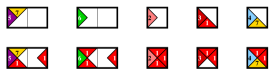
(a) tiles for variables

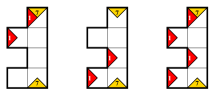
(b) clause tiles

Figure 13. Tiles for 2SAT.

Note that the modified tileset has a smaller total area, and has the same number of colors used on the boundary. Therefore as in the proof of Theorem 1.1, we apply Lemma 3.3 to conclude that $10^{6}$ rectangles suffice. ∎

7. Final remarks and open problems

7.1.

Theorem 2.1 was only announced in [GJ], referencing an unpublished preprint. Of course, now we have much stronger results.

A version of Lemma 3.2 was first announced in Levin’s original 1973 short note regarding NP-completeness [Lev], but the proof has never been published. Although we were unable to find in the literature an explicit construction for either Lemma 3.2 or, equivalently, of Theorem 2.2, we do not claim this result as ours, since it became a folklore decades ago. We include the proof for completeness, and since we need an explicit construction. An alternative proof is outlined in Subsection 7.2 below.

Let us mention that using [Oll], the number of tiles in Theorem 2.2 can be reduced to $11$, but this reduction has no effect on the number of tiles in the main theorems. Indeed, Theorem 2.2 is an immediate corollary of Lemma 3.2, which is the one needed in the proof of main theorems 1.1 and 1.2.

7.2.

Our proof of Lemma 3.2 is completely elementary and yields explicit bounds (see also Subsection 7.1). Let us sketch an alternate proof of the lemma, using a non-deterministic universal Turing machine (UTM). It was suggested to us by Cris Moore.

Fix some non-deterministic universal Turing machine ${{\mathfrak{M}}}$. Given two finite tape configurations and a natural number $t$ (in unary), it is NP-complete to decide whether ${{\mathfrak{M}}}$ transforms the first tape configuration to the second with $t$ steps of computation. Fix a finite set ${{\mathbf{W}}}$ of Wang tiles that simulate the space-time computation diagram of ${{\mathfrak{M}}}$ (see e.g. [LeP, §7]). Encode the given tape configurations as the top and bottom boundaries of a rectangular region with height $t$. This region is tileable by ${{\mathbf{W}}}$ if and only if ${{\mathfrak{M}}}$ transforms the first tape configuration to the second in precisely $t$ steps. The details are straightforward.

Note that this method also proves the counting result. Indeed, one can devise a UTM so that there is a bijective correspondence between the accepting paths of the UTM and of the Turing machine it is simulating.

The proof of Lemma 3.2 constructs a set of $23$ generalized Wang tiles ($133$ ordinary Wang tiles). However, it is possible to decrease these numbers by elementary means. After this paper was written, a modified construction by Günter Rote and the second author improves the number of generalized Wang tiles in Lemma 3.2 to $15$, which amounts to $35$ ordinary Wang tiles. With other technical improvements this does reduce the $10^{6}$ bound in Theorem 1.1 to a much friendlier $117$. The details are given in [Yang].

We do not know if this approach leads to improvements in the number of Wang tiles in the lemma, as this would depend on the smallest UTM. Given an $m$-state $n$-symbol Turing machine with $k$ instructions, the standard construction of Wang tiles to simulate such a Turing machine yields more than $nm+n+k$ tiles. As a perspective, among the smallest known UTMs, this minimum is achieved by Rogozhin’s $4$-state $6$-symbol machine with $22$ instructions, which already yields more than $52$ tiles [Rog] (see also [NW]). Unless a substantial progress is made in finding small UTMs, our elementary proof still gives better bounds.

7.3.

In the tiling literature, the original theoretical emphasis was on tileability of the plane, the decidability and aperiodicity. The problem was often stated in the equivalent language of Wang tiles [Ber, Rob2, Wang]. Unfortunately, there does not seem to be any standard treatment of the finite Wang tiling problems. Although some equivalences in the Lemma 3.1 are routine, such as the reduction in Figure 2, others seem to be new. We present full proofs for completeness.

7.4.

Historically, finite tilings were a backwater of the tiling theory, with coloring arguments being the only real tool [Gol1]. On a negative (complexity) side, originally, the tileability problem was studied for general regions, where the tiles were part of the input. The NP-completeness of this most general problem is given in [GJ, $\S$GP13]. When the set of tiles is fixed, NP-completeness was shown for general regions and various fixed small sets of tiles (see [MR] and [BNRR] building on the earlier unpublished work by Robson).

On the positive side, papers of Thurston [Thu] and Conway & Lagarias [CL] introduced the height function and the tiling group interrelated approaches. The key underlying idea is the use of combinatorial group theory applied to the boundary word of the simply connected regions, so the tilings become Van Kampen diagrams of the corresponding tiling group. This approach allowed numerous applications to perfect matchings [Cha], tile invariants [Korn, MP, Reid1], tileability [She], various local move connectivity results [KP, Rém1], classical geometric problems [Ken1], applications to colorings and mixing time [LRS], etc. More relevant to this paper, the breakthrough result by C. and R. Kenyon [KK] proved that tileability with bars of simply connected (s.c.) regions can be decided in polynomial time. This result was further extended to all pairs of rectangles by Rémila in [Rém2], and by Korn [Korn] to an infinite family of generalized dominoes. Our Main Theorem puts an end to the hopes that these results can be extended to larger sets of rectangles.

Note also that having s.c. regions gives a speed-up for polynomial problems. For example, domino tileability is a special case of perfect matching, solvable in quadratic time on all planar bipartite graphs [LP]. However, Thurston’s algorithm is linear time (in the area), for all s.c. regions (see [Cha, Thu]).

7.5.

We conjecture that in the Main Theorem (Theorem 1.1), the number of rectangles can be reduced down to 3, thus matching the lower bound (Rémila’s tileability algorithm for the case of two rectangles). As a minor supporting evidence in favor of this conjecture, let us mention that the proofs in [KK, Rém2] are crucially based on local move connectivity, which fails for three general rectangles. In the absence of algebraic methods, there seem to be no other (positive) approach to tileability.

7.6.

This result of Main Theorem can be contrasted with a large body of positive results on tiling rectangular regions with a fixed set of rectangles.

Theorem 7.1 (“Tiling rectangles with rectangles” Theorem [LMP])

For every finite set ${{\mathbf{R}}}$ of rectangular tiles, the tileability problem of an $\hskip 0.85355pt[M\times N]$ rectangle can be decided in $O(\log M+\log N)$ time.

Note that Theorem 7.1 has linear time complexity for the rectangular regions written in binary. This result is based on the pioneer results by Barnes [Bar1, Bar2] applying commutative algebra, the finite basis theorem [DK] (see also [Reid2]), and the transfer matrix method (see e.g. [Sta, Ch. 4]).

It seems, tilings of rectangles have additional structure, which general regions do not have. See e.g. [BSST, C+, Rob1] for assorted results on the subject. On the other hand, when the tiles are part of the input, deciding tileability can be NP-hard, and the proof can be used to show that counting tilings is #P-hard. Note that the results in [LMP] only discuss tileability, not counting. It would be interesting to obtain general results on the local move connectivity and hardness of counting results for tilings of rectangular regions with rectangles.

7.7.

Although counting perfect matchings in general graphs is #P-complete, for the grid graphs a Pfaffian formula gives a count for the number of domino tilings for any (not necessarily simply connected) region; this formula can be applied in polynomial time [LP] (see also [Ken2]). In a different direction, Moore and Robson [MR] conjecture that already for two bars, the problem is #P-complete for general regions. They note that the corresponding reductions in [BNRR, MR] are not parsimonious. Thus, until now, the #P-completeness was open for any finite set of rectangular tiles, even for general regions.

We make a stronger conjecture that for every tileset ${{\mathbf{T}}}$ of two bars $[1\times k]$ and $[\ell\times 1]$, where $k,\ell\geq 2$, $(k,\ell)\neq(2,2)$, the counting of tilings by ${{\mathbf{T}}}$ of simply connected regions is #P-complete. In particular, the number $10^{6}$ in Theorem 1.2 can be decreased to 2. There is no direct evidence in favor of this, except that the general combinatorial counting problems tend to be #P-complete unless there is a special algebraic formula counting them. Furthermore, when it comes to tile counting, there seem to be no direct benefit of simple connectivity of the regions, so such result is likely to be equally hard as for general regions. We refer to [Jer] for the introduction and references.

7.8.

By a simple modification of the Wang tiles, we can also get a parsimonious reduction from SAT. For that, first, we can introduce wire splitters and the NOT gate. By doing so, we remove the “cubic” and “monotone” constraints, respectively. These would play the same role as crossover tiles, and require a separate color on the boundary for each. This would also increase the set of tiles by introducing new variants for the $V$ and $L$ tiles as well. We omit the details.

We can then introduce the AND gate in a similar fashion, again with a new control color on the top and new versions of the $V$, $C$ and $L$ tiles. This gives the embedding of SAT. This reduction is parsimonious in the same way as the reduction in Theorem 1.2, which implies that the associated counting problem is also #P-complete.

Let us compute the total number of rectangles necessary for this construction. First, this would increase the number of Wang tiles from $23$ to no more than $23\cdot 8$. Then, the same argument as above gives the $10^{8}$ bound in the number of rectangular tiles. We omit the (easy) calculation and details.

7.9.

The reductions in this paper can be used to prove uniqueness results on tileability with rectangles, i.e. whether there exists a unique tiling of a region with a given set of rectangular tiles. In [BNRR], the problem was completely resolved in the case of two bars. An even simpler solution follows from [KK] in this case. Since all tilings are local move connected, taking the “minimal tiling” constructed by the algorithm in [KK] and trying all potential moves gives an easy polynomial time test. More generally, Rémila [Rém2] showed that for two general rectangles one can go from one to another with certain non-local moves which are easy to describe. Again, since he produces the “minimal tiling,” his algorithm can be used to decide unique tileability with two rectangles.

Now, our approach, via reduction from the general SAT problem (see above) shows that for a certain finite set of rectangles, uniqueness of tilings of a simply connected region is as hard as UNIQUE SAT, which is co-NP-hard and has been extensively studied [BG, VV]. This seems to be the first result of this type.

7.10.

Although Theorem 7.1 extends directly to bricks in higher dimensions [LMP], this is an exception rather than the rule. In fact, we recently showed that almost no other positive tileability results extend to higher dimensions, even Thurston’s algorithm mentioned above (see [PY]).

Acknowledgements.   We are grateful to Alex Fink, Jeff Lagarias, Leonid Levin, Cris Moore, Günter Rote, and Damien Woods for helpful conversations at various stages of this project. We also thank the anonymous referees for attentive reading and useful comments on previous versions of this paper. The first author is partially supported by the NSF and BSF grants. The second author is supported by the NSF under Grant No. DGE-0707424.

References

- [Bar1] F. W. Barnes, Algebraic theory of brick packing I, Discrete Math. 42 (1982), 7–26.
- [Bar2] F. W. Barnes, Algebraic theory of brick packing II, Discrete Math. 42 (1982), 129–144.
- [BNRR] D. Beauquier, M. Nivat, É. Rémila and M. Robson, Tiling figures of the plane with two bars, Comput. Geom. 5 (1995), 1–25.
- [Ber] R. Berger, The undecidability of the domino problem, Mem. AMS 66 (1966), 72 pp.
- [BG] A. Blass and Y. Gurevich, On the unique satisfiability problem, Inform. and Control 55 (1982), 80–88.
- [BSST] R. L. Brooks, C. A. B. Smith, A. H. Stone and W. T. Tutte, The dissection of rectangles into squares, Duke Math. J. 7 (1940), 312–340.
- [Cha] T. Chaboud, Domino tiling in planar graphs with regular and bipartite dual, Theor. Comp. Sci. 159 (1996), 137–142.
- [C+] F. R. K. Chung, E. N. Gilbert, R. L. Graham, J. B. Shearer and J. H. van Lint, Tiling rectangles with rectangles, Math. Mag. 55 (1982), no. 5, 286–291.
- [CL] J. H. Conway and J. C. Lagarias, Tilings with polyominoes and combinatorial group theory, J. Comb. Theory, Ser. A 53 (1990), 183–208.
- [CH] N. Creignou and M. Hermann, On #P-completeness of some counting problems, Research Report 2144, INRIA, 1993.
- [DK] N. G. de Bruijn and D. A. Klarner, A finite basis theorem for packing boxes with bricks, Philips Res. Rep. 30 (1975), 337∗–343∗; available at http://tinyurl.com/65g8kvr
- [GJ] M. Garey and D. S. Johnson, Computers and Intractability: A Guide to the Theory of NP-completeness, Freeman, San Francisco, CA, 1979.
- [Gol1] S. Golomb, Polyominoes, Scribners, New York, 1965.
- [Gol2] S. Golomb, Tiling with sets of polyominoes, J. Combin. Theory 9 (1970), 60–71.
- [Gon] T. F. Gonzalez, Clustering to minimize the maximum intercluster distance, Theor. Comp. Sci. 38 (1985), 293–306.
- [GS] B. Grünbaum and G. C. Shephard, Tilings and patterns, Freeman, New York, 1987.
- [Jer] M. Jerrum, Counting, sampling and integrating: algorithms and complexity, Birkhäuser, Basel, 2003.
- [Ken1] R. Kenyon, A note on tiling with integer-sided rectangles, J. Combin. Theory, Ser. A 74 (1996), 321–332.
- [Ken2] R. Kenyon, An introduction to the dimer model, in ICTP Lect. Notes XVII, Trieste, 2004.
- [KK] C. Kenyon and R. Kenyon, Tiling a polygon with rectangles, in Proc. 33rd FOCS (1992), 610–619.
- [Korn] M. Korn, Geometric and algebraic properties of polyomino tilings, MIT Ph.D. thesis, 2004; available at http://dspace.mit.edu/handle/1721.1/16628
- [KP] M. Korn and I. Pak, Tilings of rectangles with T-tetrominoes, Theor. Comp. Sci. 319 (2004), 3–27.
- [LMP] T. Lam, E. Miller and I. Pak, Tiling rectangles with rectangles, unpublished manuscript, 2005.
- [Lar] P. Laroche, Planar -in- satisfiability is NP-complete, in Proc. ASMICS Workshop on Tilings, ENS Lyon (1992).
- [Lev] L. Levin, Universal sorting problems, Problems Inf. Transm. 9 (1973), 265–266.
- [LeP] H. R. Lewis and C. H. Papadimitriou, Elements of the theory of computation, Upper Saddle River, NJ, 1998.
- [LP] L. Lovász and M. D. Plummer, Matching theory (Corrected reprint of the 1986 original), AMS, Providence, RI, 2009.
- [LRS] M. Luby, D. Randall and A. Sinclair, Markov chain algorithms for planar lattice structures, SIAM J. Comput. 31 (2001), 167–192.
- [MP] C. Moore and I. Pak, Ribbon tile invariants from the signed area, J. Combin. Theory, Ser. A 98 (2002), 1–16.
- [MRR] C. Moore, I. Rapaport and E. Remila, Tiling groups for Wang tiles, in Proc. 13th SODA (2002), 402–411.
- [MR] C. Moore and J. M. Robson, Hard tiling problems with simple tiles, Discrete Comput. Geom. 26 (2001), 573–590.
- [MuR] W. Mulzer and G. Rote, Minimum-weight triangulations is NP-hard, in Proc. 22nd SOCG (2006), 1–10.
- [NW] T. Neary and D. Woods, Four small universal Turing machines, in Proc. 5th MCU (2007), 242–254.
- [Oll] N. Ollinger, Tiling the plane with a fixed number of polyominoes, in Proc. 3rd LATA (2009), 638–647.
- [Pak] I. Pak, Tile invariants: New horizons, Theor. Comp. Sci. 303 (2003), 303–331.
- [PY] I. Pak and J. Yang, The complexity of generalized domino tilings, arXiv:1305.2154
- [Pap] C. H. Papadimitriou, Computational complexity, Addison-Wesley, Reading, MA, 1994.
- [Reid1] M. Reid, Tile homotopy groups, Enseign. Math. 49 (2003), 123–155.
- [Reid2] M. Reid, Klarner systems and tiling boxes with polyominoes, J. Combin. Theory, Ser. A 111 (2005), 89–105.
- [Rém1] É. Rémila, Tiling groups: new applications in the triangular lattice, Discrete Comput. Geom. 20 (1998), 189–204.
- [Rém2] É. Rémila, Tiling a polygon with two kinds of rectangles, Discrete Comput. Geom. 34 (2005), 313–330.
- [Rob1] P. J. Robinson, Fault-free rectangles tiled with rectangular polyominoes, in Combinatorial Mathematics IX, (Brisbane, 1981), 372–377.
- [Rob2] R. M. Robinson, Undecidability and nonperiodicity for tilings of the plane, Invent. Math. 12 (1971), 177–209.
- [Rog] Y. Rogozhin, Small universal Turing machines, Theor. Comp. Sci. 168 (1996), 215–240.
- [She] S. Sheffield, Ribbon tilings and multidimensional height functions, Trans. AMS 354 (2002), 4789–4813.
- [Sta] R. P. Stanley, Enumerative combinatorics, Vol. 1, Cambridge University Press, Cambridge, 1997.
- [Thu] W. Thurston, Conway’s tiling groups, Amer. Math. Monthly 97 (1990), 757–773.
- [Val] L. G. Valiant, The complexity of enumeration and reliability problems, SIAM J. Comput. 8 (1979), 410–421.
- [VV] L. G. Valiant and V. V. Vazirani, NP is as easy as detecting unique solutions, Theor. Comp. Sci. 47 (1986), 85–93.
- [Wang] H. Wang, Games, logic and computers, in Scientific American (Nov. 1965), 98–106.
- [Yang] J. Yang, Ph.D. thesis, available at http://tinyurl.com/d4a89ns