Cohomogeneity One Coassociative Submanifolds in the Bundle of Anti-self-dual 2-forms over the 4-sphere

Abstract

Coassociative submanifolds are 4-dimensional calibrated submanifolds in $G_{2}$-manifolds. In this paper, we construct explicit examples of coassociative submanifolds in $\Lambda^{2}_{-}S^{4}$, which is the complete $G_{2}$-manifold constructed by Bryant and Salamon. Classifying the Lie groups which have 3- or 4-dimensional orbits, we show that the only homogeneous coassociative submanifold is the zero section of $\Lambda^{2}_{-}S^{4}$ up to the automorphisms and construct many cohomogeneity one examples explicitly. In particular, we obtain examples of non-compact coassociative submanifolds with conical singularities and their desingularizations.

1 Introduction

In 1996, Strominger, Yau and Zaslow [21] presented a conjecture explaining mirror symmetry of compact Calabi-Yau 3-folds in terms of dual fibrations by special Lagrangian 3-tori, including singular fibers. Analogously, fibrations of coassociative 4-folds in compact $G_{2}$-manifolds are expected to play the same role as special Lagrangian fibrations in Calabi-Yau manifolds. In this paper, we focus on the construction of coassociative 4-folds in a non-compact $G_{2}$-manifold. By constructing these examples, we will gain a greater understanding of coassociative geometry and local models for coassociative submanifolds in compact $G_{2}$-manifolds.

In $\mathbb{R}^{7}$, Harvey and Lawson gave ${\rm SU}(2)$-invariant coassociative submanifolds in their pioneering paper [6]. Lotay [14, 15] constructed 2-ruled examples and ones with the $T^{2}\times\mathbb{R}_{>0}$ symmetries using evolution equations. Fox [4] obtained a family of non-2-ruled, non-conical examples from a 2-ruled coassociative cone. Ionel, Karigiannis and Min-Oo [11] gave examples in $\Lambda^{2}_{-}\mathbb{R}^{4}\cong\mathbb{R}^{7}$, which are the total spaces of certain rank 2 subbundles over immersed surfaces in $\mathbb{R}^{4}$. Karigiannis and Leung [12] generalized this method by twisting the bundles by a special section of a complementary bundle. Karigiannis and Min-Oo [13] applied the method in [11] to $\Lambda^{2}_{-}S^{4}$ and $\Lambda^{2}_{-}\mathbb{C}P^{2}$ and obtained some examples. Here, $\Lambda^{2}_{-}S^{4}$ and $\Lambda^{2}_{-}\mathbb{C}P^{2}$ admit complete $G_{2}$-metrics constructed by Bryant and Salamon [2].

In this paper, we focus on the case of $\Lambda^{2}_{-}S^{4}$ and construct many explicit examples of coassociative submanifolds in $\Lambda^{2}_{-}S^{4}$. There exists a family of torsion-free $G_{2}$-structures $\{(\varphi_{\lambda},g_{\lambda})\}_{\lambda>0}$ on $\Lambda^{2}_{-}S^{4}$ (Proposition 3.1). For each $\lambda>0$, the automorphism group of $(\Lambda^{2}_{-}S^{4},\varphi_{\lambda},g_{\lambda})$ is ${\rm SO}(5)$ acting on $\Lambda^{2}_{-}S^{4}$ by the lift of the standard action on $S^{4}$ ([19]).

First, by classifying the Lie subgroups of ${\rm SO}(5)$ which have 4-dimensional orbits in $\Lambda^{2}_{-}S^{4}$, we obtain the following result.

Theorem 1.1.

Let $\{(\varphi_{\lambda},g_{\lambda})\}_{\lambda>0}$ be the family of torsion-free $G_{2}$-structures on $\Lambda^{2}_{-}S^{4}$ in Proposition 3.1. For each $\lambda>0$, every homogeneous coassociative submanifold in $(\Lambda^{2}_{-}S^{4},\varphi_{\lambda},g_{\lambda})$ is congruent under the action of ${\rm SO}(5)$ to the zero section $S^{4}\subset\Lambda^{2}_{-}S^{4}$.

Next, we prove that the Lie subgroup of ${\rm SO}(5)$ which have 3-dimensional orbits in $\Lambda^{2}_{-}S^{4}$ is one of the following (Proposition 4.15).

$${\rm SO}(4) ={\rm SO}(4)\times\{1\},\qquad {\rm SO}(3)\times{\rm SO}(2),\qquad{\rm U}(2),\ {\rm SU}(2)\subset{\rm SO}(4)\times\{1\},$$

$${\rm SO}(3) ={\rm SO}(3)\times\{I_{2}\},\qquad {\rm SO}(3)\mbox{ acting irreducibly on }\mathbb{R}^{5}.$$

We derive O.D.E.s which give coassociative submanifolds by the cohomogeneity one method of Hsiang and Lawson [10] in each case. In many cases, O.D.E.s are solved explicitly and we obtain the following new examples.

Let $(x_{1},x_{2},x_{3},x_{4},x_{5})$ be standard coordinates of $\mathbb{R}^{5}$ and regard $S^{4}$ as the unit sphere in $\mathbb{R}^{5}$. Let $(a_{1},a_{2},a_{3})$ be the local fiber coordinates of $\Lambda^{2}_{-}S^{4}$ by choosing a local frame for $\Lambda^{2}_{-}S^{4}$ as in Section 3.2.1.

Theorem 1.2 (Case of ${\rm SO}(3)\times{\rm SO}(2)$).

Let ${\rm SO}(3)\times{\rm SO}(2)$ act on $\Lambda^{2}_{-}S^{4}$ by the lift of the standard ${\rm SO}(3)\times{\rm SO}(2)$-action on $S^{4}$. For any $C\in\mathbb{R}$, set

$$M_{C}={\rm SO}(3)\times{\rm SO}(2)\cdot\left\{\left({}^{t}\!(x_{1},0,0,\sqrt{1-x_{1}^{2}},0),{}^{t}\!(a_{1},0,0)\right);\begin{array}[]{c}G(a_{1},x_{1})=C,\\ a_{1}\in\mathbb{R},0<x_{1}\leq 1\end{array}\right\},$$

where $G(a_{1},x_{1})$ is defined in (5.2). Then $M_{C}$ is coassociative and it is homeomorphic to

$$\left\{\begin{array}[]{ll}(S^{2}\times\mathbb{R}^{2})\sqcup(S^{2}\times S^{1}\times\mathbb{R}_{>0})&\qquad\mbox{for }\ C\neq 0,\\ S^{4}\sqcup(S^{2}\times S^{1}\times\mathbb{R}_{>0})\sqcup(S^{2}\times S^{1}\times\mathbb{R}_{>0})&\qquad\mbox{for }\ C=0,\end{array}\right.$$

where $S^{4}$ is the zero section of $\Lambda^{2}_{-}S^{4}$.

Theorem 1.3 (Case of ${\rm SU}(2)\subset{\rm SO}(4)\times\{1\}$).

Let ${\rm SU}(2)$ act on $\Lambda^{2}_{-}S^{4}$ by the lift of the standard action of ${\rm SU}(2)\subset{\rm SO}(4)\times\{1\}$ on $S^{4}$. For any $C\in\mathbb{R}$ and $v\in S^{2}\subset\mathbb{R}^{3}$, set

$$M_{C,v}:={\rm SU}(2)\cdot\left\{\left({}^{t}\!(\sqrt{1-x_{5}^{2}},0,0,0,x_{5}),rv\right);F(r,x_{5})=C,r\geq 0,-1\leq x_{5}\leq 1\right\},$$

where $F(r,x_{5})$ is defined in (5.24). Then $M_{C,v}$ is coassociative and it is homeomorphic to

$$\left\{\begin{array}[]{ll}\mathbb{R}^{4}&\qquad\mbox{for }\ C>0,\\ S^{4}\sqcup(S^{3}\times\mathbb{R}_{>0})&\qquad\mbox{for }\ C=0,\\ \mathcal{O}_{\mathbb{C}P^{1}}(-1)&\qquad\mbox{for }\ C<0,\end{array}\right.$$

where $S^{4}$ is the zero section of $\Lambda^{2}_{-}S^{4}$ and $\mathcal{O}_{\mathbb{C}P^{1}}(-1)$ is the tautological line bundle over $\mathbb{C}P^{1}\cong S^{2}$.

By using the stereographic local coordinates, the ${\rm SU}(2)$-action is described as in the case of $\mathbb{R}^{7}$. See (5.25). In this sense, the above example is an analogue of an ${\rm SU}(2)$-invariant coassociative submanifold in $\mathbb{R}^{7}$ given by Harvey and Lawson [6].

Theorem 1.4 (Case of ${\rm SO}(3)={\rm SO}(3)\times\{I_{2}\}$).

Let ${\rm SO}(3)$ act on $\Lambda^{2}_{-}S^{4}$ by the lift of the standard ${\rm SO}(3)={\rm SO}(3)\times\{I_{2}\}$-action on $S^{4}$. For $C,D\geq 0$ and $E\in\mathbb{R}$, set

$$M_{C,D,E}={\rm SO}(3)\cdot\left\{({}^{t}\!(x_{1},0,0,x_{4},x_{5}),{}^{t}\!(a_{1},a_{2},0));\begin{array}[]{c}x_{4}^{4}(\lambda+r^{2})=C,\\ x_{5}^{4}(\lambda+r^{2})=D,\\ a_{1}x_{1}=E\end{array}\right\}.$$

Then $M_{C,D,E}$ is coassociative and the topology of $M_{C,D,E}$ is given in Lemma 5.12. In particular, we obtain examples of non-compact coassociative submanifolds with conical singularities for $(C,D)\neq(0,0),E=0,\sqrt{C}+\sqrt{D}=\sqrt{\lambda}$ and their desingularizations.

Theorem 1.5 (Case of irreducible ${\rm SO}(3)$).

Let ${\rm SO}(3)$ act on $\Lambda^{2}_{-}S^{4}$ by the lift of the irreducible ${\rm SO}(3)$-action on $S^{4}$. Let $x_{1}(t),x_{5}(t),a_{1}(t),a_{2}(t),a_{3}(t)$ be smooth functions on an open interval $I\subset\mathbb{R}$ satisfying $0\leq x_{1}(t)\leq\sqrt{3}/2,|x_{5}(t)|<1/2,x_{1}^{2}(t)+x_{5}^{2}(t)=1$,

$$4\left\{(2\sqrt{3}x_{1}+4x_{5}+1)\dot{x}_{5}+\sqrt{3}(2x_{5}-1)\dot{x}_{1}\right\}a_{1}+8x_{1}(-x_{1}+\sqrt{3}x_{5})\dot{a}_{1}$$

$$-(\sqrt{3}x_{1}+x_{5}+1)(1-2x_{5})a_{1}\frac{d}{dt}\log(\lambda+r^{2}) =0,$$

$$4\left\{(2\sqrt{3}x_{1}-4x_{5}-1)\dot{x}_{5}+\sqrt{3}(2x_{5}-1)\dot{x}_{1}\right\}a_{2}+8x_{1}(x_{1}+\sqrt{3}x_{5})\dot{a}_{2}$$

$$+(-\sqrt{3}x_{1}+x_{5}+1)(1-2x_{5})a_{2}\frac{d}{dt}\log(\lambda+r^{2}) =0,$$

$$4\left\{-(x_{5}+1)\dot{x}_{5}+3x_{1}\dot{x}_{1}\right\}a_{3}+2(x_{1}^{2}-3x_{5}^{2})\dot{a}_{3}$$

$$+(1+x_{5})(1-2x_{5})a_{3}\frac{d}{dt}\log(\lambda+r^{2}) =0,$$

where $r^{2}(t)=\sum_{j=1}^{3}a_{j}^{2}(t)$ and $\dot{x}_{1}=dx_{1}/dt$, etc. Then

$${\rm SO}(3)\cdot\left\{({}^{t}\!(x_{1}(t),0,0,0,x_{5}(t)),{}^{t}\!(a_{1}(t),a_{2}(t),a_{3}(t)));t\in I\right\},$$

is a coassociative submanifold invariant under the irreducible ${\rm SO}(3)$-action.

This paper is organized as follows. In Section 2, we review the fundamental facts of calibrated geometry and $G_{2}$ geometry and introduce the cohomogeneity one method of Hsiang and Lawson [10]. In Section 3, we introduce the $G_{2}$-structure on $\Lambda^{2}_{-}S^{4}$ given by Bryant and Salamon [2]. In Section 4, we classify the connected closed subgroups of ${\rm SO}(5)$, which is the automorphism group of the $G_{2}$-manifold $\Lambda^{2}_{-}S^{4}$, and study their orbits. Classifying Lie subgroups which have 3- or 4-dimensional orbits, we prove Theorem 1.1. In Section 5, according to the classification in Section 4, we construct cohomogeneity one coassociative submanifolds and prove Theorems 1.2, 1.3, 1.4 and 1.5.

Acknowledgements: The author is very grateful to Professor Katsuya Mashimo for his useful advice about the representation theory. He would like to thank the referees for the careful reading of an earlier version of this paper and useful comments on it.

2 Preliminaries

Definition 2.1.

Define a 3-form $\varphi_{0}$ on $\mathbb{R}^{7}$ by

$$\varphi_{0}=e^{123}+e^{145}-e^{167}+e^{246}+e^{257}+e^{347}-e^{356},$$ (2.1)

where $(e^{1},\cdots,e^{7})$ is the standard dual basis on $\mathbb{R}^{7}$ and wedge signs are omitted. The stabilizer of $\varphi_{0}$ is the exceptional Lie group $G_{2}$:

$$G_{2}=\{g\in GL(7,\mathbb{R});g^{*}\varphi_{0}=\varphi_{0}\}.$$

This is a 14-dimensional compact simply-connected simple Lie group.

The Lie group $G_{2}$ also fixes the standard metric $g_{0}=\sum^{7}_{i=1}(e^{i})^{2}$, the orientation on $\mathbb{R}^{7}$ and the 4-form

$$*\varphi_{0}=e^{4567}+e^{2367}-e^{2345}+e^{1357}+e^{1346}+e^{1256}-e^{1247},$$

where $*$ means the Hodge dual. They are uniquely determined by $\varphi_{0}$ via

$$-6g_{0}(v_{1},v_{2}){\rm vol}_{g_{0}}=i(v_{1})\varphi_{0}\wedge i(v_{2})\varphi_{0}\wedge\varphi_{0},$$ (2.2)

where ${\rm vol}_{g_{0}}$ is the volume form of $g_{0}$, $i(\cdot)$ is the interior product, and $v_{i}\in T(\mathbb{R}^{7})$.

Definition 2.2.

Let $Y$ be a 7-dimensional oriented manifold and $\varphi$ be a 3-form on $Y$. A 3-form $\varphi$ is called a $G_{2}$-structure on $Y$ if for each $y\in Y$, there exists an oriented isomorphism between $T_{y}Y$ and $\mathbb{R}^{7}$ identifying $\varphi_{y}$ with $\varphi_{0}$. From (2.2), $\varphi$ induces the metric $g$ on $Y$, volume form on $Y$ and $*\varphi\in\Omega^{4}(Y)$.

A $G_{2}$-structure $\varphi$ is called torsion-free if $\varphi$ is closed and coclosed: $d\varphi=d*\varphi=0$. We call a triple $(Y,\varphi,g)$ a $G_{2}$-manifold if $\varphi\in\Omega^{3}(Y)$ is a torsion-free $G_{2}$-structure on $Y$ and $g$ is the associated metric.

Lemma 2.3 ([3]).

Let $(Y,\varphi,g)$ be a manifold with a $G_{2}$-structure. Then the holonomy group of $g$ is contained in $G_{2}$ if and only if $d\varphi=d*\varphi=0$.

Recall the notion of a calibration introduced by Harvey and Lawson [6].

Definition 2.4.

Let $(Y,g)$ be an $n$-dimensional Riemannian manifold. A closed $k$-form $\varphi$ on $Y$, where $1\leq k\leq n$, is called a calibration on $Y$ if $\varphi|_{V}\leq{\rm vol}_{V}$ for each point $p\in Y$ and every oriented $k$-dimensional subspace $V\subset T_{p}Y$. We say that an oriented $k$-dimensional submanifold $L$ of $Y$ is a calibrated submanifold of $Y$ (or calibrated by $\varphi$) if $\varphi|_{TL}={\rm vol}_{L}.$

There are canonical calibrations on a $G_{2}$-manifold.

Lemma 2.5 ([6]).

Let $(Y,\varphi,g)$ be a $G_{2}$-manifold. Then the $G_{2}$-structure $\varphi$ and its Hodge dual $*\varphi$ define calibrations on Y.

Definition 2.6 ([6]).

An oriented 3-dimensional submanifold is called an associative submanifold of $Y$ if it is calibrated by $\varphi$. An oriented 4-dimensional submanifold is called a coassociative submanifold of $Y$ if it is calibrated by $*\varphi$.

Lemma 2.7 ([6]).

If $L\subset Y$ is an oriented 4-dimensional submanifold, then $L$ is a coassociative submanifold of Y up to a possible change of orientation for $L$ if and only if $\varphi|_{TL}=0$.

This description is often more useful and easier to work with.

2.1 Cohomogeneity one method

Let $L$ be a coassociative submanifold of a $G_{2}$-manifold $(Y,\varphi,g)$. The symmetry group $K$ of $L$ is defined to be the Lie subgroup of the automorphism group which fixes $L$. If the principal orbits of $K$ are of codimension one in $L$, we call $L$ a cohomogeneity one coassociative submanifold. The action of $K$ on $L$ is called a cohomogeneity one action.

Coassociative submanifolds are defined by first order nonlinear P.D.E.s, which are difficult to solve in general. By the cohomogeneity one action of the Lie group, we reduce the P.D.E.s of the coassociative condition to nonlinear O.D.E.s, which are easier to solve. This method was introduced in [10] for minimal submanifolds. We give a summary in our coassociative settings based on [8].

Lemma 2.8.

Let $(Y,\varphi,g)$ be a $G_{2}$-manifold and $G$ be a Lie subgroup of the automorphism group of $(Y,\varphi,g)$. Let $\Sigma\subset Y$ be a subset which is transverse to the $G$-orbits and satisfies $G\cdot\Sigma=Y$. Suppose that $G$ has 3-dimensional orbits on $Y$.

Then the solution of the first order nonlinear O.D.E.s $\varphi|_{G\cdot{\rm Image}(c)}=0$, where $c:I\rightarrow\Sigma$ is a path and $I\subset\mathbb{R}$ is an open interval, gives a $G$-invariant coassociative submanifold $G\cdot{\rm Image}(c)$.

Note that there is a similar construction by using evolution equations. This method was introduced by Lotay [15] for associative, coassociative and Cayley submanifolds.

3 Geometry in $\Lambda^{2}_{-}S^{4}$

3.1 $G_{2}$-structure on $\Lambda^{2}_{-}S^{4}$

We introduce the complete metric on the bundle $\Lambda^{2}_{-}S^{4}$ of anti-self-dual 2-forms over the 4-sphere $S^{4}$ obtained by Bryant and Salamon [2]. We also refer to [13, 20]. Since $\Lambda^{2}_{-}S^{4}$ has a connection induced by the Levi Civita connection on $S^{4}$, the tangent space $T_{\omega}(\Lambda^{2}_{-}S^{4})$ has a canonical splitting $T_{\omega}(\Lambda^{2}_{-}S^{4})\cong\mathcal{H}_{\omega}\oplus\mathcal{V}_{\omega}$ into horizontal and vertical subspaces for each $\omega\in\Lambda^{2}_{-}S^{4}$.

Proposition 3.1 (Bryant and Salamon [2]).

For $\lambda>0$, define the 3-form $\varphi_{\lambda}\in\Omega^{3}(\Lambda^{2}_{-}S^{4})$ and the metric $g_{\lambda}$ on $\Lambda^{2}_{-}S^{4}$ by

$$\varphi_{\lambda}=2s_{\lambda}d\tau+\frac{1}{s_{\lambda}^{3}}{\rm vol_{\mathcal{V}}},\qquad g_{\lambda}=2s_{\lambda}^{2}g_{\mathcal{H}}+\frac{1}{s_{\lambda}^{2}}g_{\mathcal{V}},$$

where $s_{\lambda}=(\lambda+r^{2})^{1/4}$, $r$ is the distance function measured by the fiber metric induced by that on $S^{4}$, $\tau$ is a tautological 2-form and ${\rm vol_{\mathcal{V}}}$ is the volume form of $g_{\mathcal{V}}$ on the vertical fiber.

Then for each $\lambda>0$, $(\Lambda^{2}_{-}S^{4},\varphi_{\lambda},g_{\lambda})$ is a $G_{2}$-manifold and $g_{\lambda}$ is the complete metric with holonomy equal to $G_{2}$.

Remark 3.2.

A complete holonomy $G_{2}$ metric is constructed not only on $\Lambda^{2}_{-}S^{4}$ but also on $\Lambda^{2}_{-}\mathbb{C}P^{2}$ in [2]. Of course, we can also apply the method in Section 2.1 to $\Lambda^{2}_{-}\mathbb{C}P^{2}$ and construct examples in theory.

By using a local frame, $\varphi_{\lambda}$ is described as follows. Let $\{e^{1},e^{2},e^{3},e^{4}\}$ be a local oriented orthonormal coframe with respect to the standard metric and the standard orientation on $S^{4}$. Define 2-forms $\omega_{i}$ on $S^{4}$ by

$$\omega_{1}=e^{12}-e^{34},\qquad\omega_{2}=e^{13}-e^{42},\qquad\omega_{3}=e^{14}-e^{23}.$$

Then $\{\omega_{1},\omega_{2},\omega_{3}\}$ is a local oriented coframe of $\Lambda^{2}_{-}S^{4}$, which is orthogonal but not normalized to unit length, and induces the local fiber coordinates $(a_{1},a_{2},a_{3})$ of $\Lambda^{2}_{-}S^{4}$. Write $\nabla\omega_{i}=\sum_{j=1}^{3}\gamma_{ij}\otimes\omega_{j}$, where $\nabla$ is the induced connection from the Levi-Civita connection of the standard metric on $S^{4}$ and $\gamma_{ij}$ is a local 1-form. Let $\pi:\Lambda^{2}_{-}S^{4}\rightarrow S^{4}$ be the projection. Denoting $b_{i}=da_{i}+\sum_{j=1}^{3}a_{j}\pi^{*}\gamma_{ji}$, we have

$$r^{2}=\sum_{i=1}^{3}a_{i}^{2},\qquad\tau=\sum_{i=1}^{3}a_{i}\pi^{*}\omega_{i},\qquad d\tau=\sum_{i=1}^{3}b_{i}\wedge\pi^{*}\omega_{i},\qquad{\rm vol}_{\mathcal{V}}=b_{123},$$

where $b_{123}=b_{1}\wedge b_{2}\wedge b_{3}$. Thus the $G_{2}$-structure $\varphi_{\lambda}$ is described as

$$\varphi_{\lambda}=2s_{\lambda}\sum_{i=1}^{3}b_{i}\wedge\pi^{*}\omega_{i}+\frac{1}{s_{\lambda}^{3}}b_{123}.$$ (3.1)

Remark 3.3.

For $\lambda=0$, the metric $g_{0}$ is a cone metric on $\Lambda^{2}_{-}S^{4}-\{\mbox{zero section}\}\cong\mathbb{C}P^{3}\times\mathbb{R}_{>0}$. The metric $g_{\mathbb{C}P^{3}}$ on $\mathbb{C}P^{3}$ induced from $g_{0}$ is not the standard metric, but a 3-symmetric Einstein, non-Kähler metric. The metric $g_{0}$ is not complete because of the singularity at 0, while its holonomy group is equal to $G_{2}$.

3.2 Local frames of $\Lambda^{2}_{-}S^{4}$

We use the following local frames of $\Lambda^{2}_{-}S^{4}$ for the convenience of computations.

3.2.1 Local frame on $S^{4}-\{x_{5}=\pm 1\}$

Define a local oriented orthonormal frame $\{e_{1},e_{2},e_{3},e_{4}\}$ on $S^{4}-\{x_{5}=\pm 1\}$ by

$$(e_{1},e_{2},e_{3},e_{4})=\frac{1}{\sqrt{1-x_{5}^{2}}}\left(\left(\begin{array}[]{c}-x_{2}\\ x_{1}\\ -x_{4}\\ x_{3}\\ 0\end{array}\right),\left(\begin{array}[]{c}-x_{3}\\ x_{4}\\ x_{1}\\ -x_{2}\\ 0\end{array}\right),\left(\begin{array}[]{c}-x_{4}\\ -x_{3}\\ x_{2}\\ x_{1}\\ 0\end{array}\right),\left(\begin{array}[]{c}-x_{1}x_{5}\\ -x_{2}x_{5}\\ -x_{3}x_{5}\\ -x_{4}x_{5}\\ 1-x_{5}^{2}\end{array}\right)\right).$$

Let $\{e^{i}\}$ be the dual coframe of $\{e_{i}\}$. Set the local orthogonal trivialization $\{\omega_{1},\omega_{2},\omega_{3}\}=\{e^{12}-e^{34},e^{13}-e^{42},e^{14}-e^{23}\}$ of $\Lambda^{2}_{-}S^{4}$ and denote by $(a_{1},a_{2},a_{3})$ local fiber coordinates with respect to $\{\omega_{1},\omega_{2},\omega_{3}\}$. Recall 1-forms $\gamma_{ij}$ and $b_{i}$ are defined by $\nabla\omega_{i}=\sum_{j=1}^{3}\gamma_{ij}\otimes\omega_{j}$, $b_{i}=da_{i}+\sum_{j=1}^{3}a_{j}\pi^{*}\gamma_{ji}$. Denote by $\nabla^{S^{4}}$ the Levi-Civita connection of the standard metric on $S^{4}$. Then we see the following by a straightforward computation.

Lemma 3.4.

$$(\nabla_{e_{i}}^{S^{4}}e^{j}) =\frac{1}{\sqrt{1-x_{5}^{2}}}\left(\begin{array}[]{cccc}x_{5}e^{4}&-e^{3}&e^{2}&-x_{5}e^{1}\\ e^{3}&x_{5}e^{4}&-e^{1}&-x_{5}e^{2}\\ -e^{2}&e^{1}&x_{5}e^{4}&-x_{5}e^{3}\\ 0&0&0&0\\ \end{array}\right),$$

$$(\gamma_{ij}) =\frac{1+x_{5}}{\sqrt{1-x_{5}^{2}}}\left(\begin{array}[]{ccc}0&-e^{1}&e^{2}\\ e^{1}&0&e^{3}\\ -e^{2}&-e^{3}&0\end{array}\right),$$

$$\left(\begin{array}[]{c}b_{1}\\ b_{2}\\ b_{3}\end{array}\right) =\left(\begin{array}[]{c}da_{1}\\ da_{2}\\ da_{3}\end{array}\right)+\frac{1+x_{5}}{\sqrt{1-x_{5}^{2}}}\left(\begin{array}[]{c}a_{2}e^{1}-a_{3}e^{2}\\ -a_{1}e^{1}-a_{3}e^{3}\\ a_{1}e^{2}+a_{2}e^{3}\end{array}\right).$$

3.2.2 Frame at $\underline{p_{0}}={}^{t}\!(0,0,0,0,\pm 1)$

Set an oriented orthonormal basis $\{f_{1},f_{2},f_{3},f_{4}\}$ of $T_{\underline{p_{0}}}S^{4}$ by

$$f_{1} ={}^{t}\!(1,0,0,0,0),\qquad f_{2}={}^{t}\!(0,1,0,0,0),$$

$$f_{3} ={}^{t}\!(0,0,1,0,0),\qquad f_{4}={}^{t}\!(0,0,0,\pm 1,0).$$

Note that the induced orientation on $T_{{}^{t}\!(0,0,0,0,1)}S^{4}$ is opposite to that of $T_{{}^{t}\!(0,0,0,0,-1)}S^{4}$. Let $\{f^{i}\}$ be the dual coframe of $\{f_{i}\}$. Then a basis $\{\Omega_{1},\Omega_{2},\Omega_{3}\}=\{f^{12}-f^{34},f^{13}-f^{42},f^{14}-f^{23}\}$ of $\Lambda^{2}_{-}S^{4}|_{\underline{p_{0}}}$ gives fiber coordinates $(A_{1},A_{2},A_{3})$ of $\Lambda^{2}_{-}S^{4}|_{\underline{p_{0}}}$.

4 Orbits of closed Lie subgroups of ${\rm SO}(5)$

For each $\lambda>0$, the automorphism group of $(\Lambda^{2}_{-}S^{4},\varphi_{\lambda},g_{\lambda})$ is ${\rm SO}(5)$ acting on $\Lambda^{2}_{-}S^{4}$ as the lift of the standard action on $S^{4}$ ([19]). We study the Lie subgroups of ${\rm SO}(5)$ to obtain homogeneous and cohomogeneity one coassociative submanifolds. By the classification of compact Lie groups, we obtain the following.

Lemma 4.1.

The $k$-dimensional connected closed Lie subgroup of ${\rm SO}(5)$, where $3\leq k\leq 10$, is one of the following.

$$\begin{array}[]{ll}{\rm SO}(5),\\ {\rm SO}(4)={\rm SO}(4)\times\{1\},\\ {\rm SO}(3)\times{\rm SO}(2),\\ {\rm U}(2)\subset{\rm SO}(4)\times\{1\},\\ \end{array}\hskip 28.45274pt\begin{array}[]{ll}{\rm SU}(2)\subset{\rm SO}(4)\times\{1\},\\ {\rm SO}(3)={\rm SO}(3)\times\{I_{2}\},\\ {\rm SO}(3)\mbox{ acting irreducibly on }\mathbb{R}^{5}.\end{array}$$

The proof is given in Appendix B. According to Lemma 4.1, we study the orbits on $\Lambda^{2}_{-}S^{4}$ of Lie subgroups of ${\rm SO}(5)$ above.

4.1 ${\rm SO}(4)={\rm SO}(4)\times\{1\}$ and ${\rm SO}(5)$-actions

In this subsection, We consider both the ${\rm SO}(4)={\rm SO}(4)\times\{1\}$ and the ${\rm SO}(5)$-orbits.

Lemma 4.2 (Orbits of the ${\rm SO}(4)$-action).

By the ${\rm SO}(4)$-action, any point in $\Lambda^{2}_{-}S^{4}$ is mapped to a point in the fiber of $\underline{p_{0}}={}^{t}\!(x_{1},0,0,0,x_{5})$ where $x_{1}\geq 0$. The ${\rm SO}(4)$-orbit through $p_{0}\in\Lambda^{2}_{-}S^{4}|_{\underline{p_{0}}}$ is diffeomorphic to

$$\left\{\begin{array}[]{ll}{\rm SO}(4)/{\rm SO}(2)&\qquad\mbox{for }\ x_{1}>0,p_{0}\neq 0,\\ S^{3}&\qquad\mbox{for }\ x_{1}>0,p_{0}=0,\\ S^{2}&\qquad\mbox{for }\ x_{5}=\pm 1,p_{0}\neq 0,\\ &\qquad\mbox{for }\ x_{5}=\pm 1,p_{0}=0.\end{array}\right.$$

Corollary 4.3.

Let $\mathcal{O}$ be an ${\rm SO}(5)$-orbit. Then $\dim\mathcal{O}\leq 4$ if and only if $\mathcal{O}$ is the zero section $S^{4}$.

Proof of Lemma 4.2.

It is obvious that any point in $\Lambda^{2}_{-}S^{4}$ is congruent to a point in the fiber of $\underline{p_{0}}={}^{t}\!(x_{1},0,0,0,x_{5})$, where $x_{1}\geq 0$, by the ${\rm SO}(4)={\rm SO}(4)\times\{1\}$-action.

Suppose that $x_{1}>0$. Since the stabilizer of the ${\rm SO}(4)$-action on $S^{4}$ at $\underline{p_{0}}$ is ${\rm SO}(3)=\{1\}\times{\rm SO}(3)\times\{1\}\subset{\rm SO}(5)$, we consider this ${\rm SO}(3)$-action on $\Lambda^{2}_{-}S^{4}|_{\underline{p_{0}}}.$ Use the notation in Section 3.2.1. Since $x_{2}=x_{3}=x_{4}=0$, the action of $g=(g_{ij})\in{\rm SO}(3)=\{1\}\times{\rm SO}(3)\times\{1\}$ is given by

$$g_{*}e_{i}=\sum_{j=1}^{3}g_{ji}e_{j}\ \mbox{ for }i=1,2,3,\qquad g_{*}e_{4}=e_{4}$$

at $\underline{p_{0}}$. Then the induced action of $g=(g_{ij})\in{\rm SO}(3)$ on $\Lambda^{2}_{-}S^{4}|_{\underline{p_{0}}}$ is described as

$$\left(\begin{array}[]{c}a_{1}\\ a_{2}\\ a_{3}\\ \end{array}\right)\mapsto\left(\begin{array}[]{ccc}g_{33}&-g_{32}&-g_{31}\\ -g_{23}&g_{22}&g_{21}\\ -g_{13}&g_{12}&g_{11}\\ \end{array}\right)\left(\begin{array}[]{c}a_{1}\\ a_{2}\\ a_{3}\\ \end{array}\right).$$

Thus the stabilizer of the ${\rm SO}(4)$-action on $\Lambda^{2}_{-}S^{4}$ at $p_{0}=({}^{t}\!(x_{1},0,0,0,x_{5}),{}^{t}\!(a_{1},a_{2},a_{3}))$ is ${\rm SO}(2)$ when ${}^{t}\!(a_{1},a_{2},a_{3})\neq 0$. It is ${\rm SO}(3)$ when ${}^{t}\!(a_{1},a_{2},a_{3})=0$.

Next, suppose that $x_{5}=\pm 1$. Then the stabilizer of the ${\rm SO}(4)$-action on $S^{4}$ at $\underline{p_{0}}={}^{t}\!(0,0,0,0,\pm 1)$ is ${\rm SO}(4)$. By using the frame in Section 3.2.2, the induced action of ${\rm SO}(4)$ on $\Lambda^{2}_{-}S^{4}|_{\underline{p_{0}}}$ is equivalent to that of ${\rm SO}(4)=({\rm Sp}(1)\times{\rm Sp}(1))/\mathbb{Z}_{2}$ on $\Lambda^{2}_{\mp}\mathbb{R}^{4}=\mathbb{R}^{3}={\rm Im}\mathbb{H}$, which is described as

$$[(p,q)]\cdot a =qa\overline{q}\qquad\mbox{ if }\underline{p_{0}}={}^{t}\!(0,0,0,0,1),$$

$$[(p,q)]\cdot a =pa\overline{p}\qquad\mbox{ if }\underline{p_{0}}={}^{t}\!(0,0,0,0,-1).$$

This is the standard action of ${\rm Sp}(1)/\mathbb{Z}_{2}={\rm SO}(3)$ on $\mathbb{R}^{3}$, and hence we obtain the lemma. ∎

Proof of Corollary 4.3.

It is obvious that any point in $\Lambda^{2}_{-}S^{4}$ is congruent to a point in the fiber of $\underline{p_{0}}={}^{t}\!(1,0,0,0,0)$ by the ${\rm SO}(5)$-action. By Lemma 4.2, the subgroup ${\rm SO}(4)\subset{\rm SO}(5)$ has 5-dimensional orbits on each point of $\Lambda^{2}_{-}S^{4}|_{\underline{p_{0}}}-\{0\}$. Hence $\mathcal{O}$ must be the zero section $S^{4}$. ∎

4.2 ${\rm SO}(3)\times{\rm SO}(2)$-action

Use the notation in Section 3.2.1.

Lemma 4.4 (Orbits of the ${\rm SO}(3)\times{\rm SO}(2)$-action).

By the ${\rm SO}(3)\times{\rm SO}(2)$-action, any point in $\Lambda^{2}_{-}S^{4}$ is mapped to a point in the fiber of $\underline{p_{0}}={}^{t}\!(x_{1},0,0,x_{4},0)\in S^{4}$, where $x_{1},x_{4}\geq 0$. The ${\rm SO}(3)\times{\rm SO}(2)$-orbit through $p_{0}=({}^{t}\!(x_{1},0,0,x_{4},0),{}^{t}\!(a_{1},a_{2},a_{3}))\in\Lambda^{2}_{-}S^{4}|_{\underline{p_{0}}}$ is diffeomorphic to

$$\left\{\begin{array}[]{ll}{\rm SO}(3)\times{\rm SO}(2)&\qquad\mbox{for }\ 0<x_{1}<1,(a_{2},a_{3})\neq 0,\\ S^{2}\times S^{1}&\qquad\mbox{for }\ 0<x_{1}<1,(a_{2},a_{3})=0,\\ ({\rm SO}(3)\times{\rm SO}(2))/{\rm SO}(2)&\qquad\mbox{for }\ x_{1}=1,(a_{2},a_{3})\neq 0,\\ S^{2}&\qquad\mbox{for }\ x_{1}=1,(a_{2},a_{3})=0,\\ S^{2}\times S^{1}&\qquad\mbox{for }\ x_{1}=0,(a_{1},a_{2},a_{3})\neq 0,\\ S^{1}&\qquad\mbox{for }\ x_{1}=0,(a_{1},a_{2},a_{3})=0.\end{array}\right.$$

When $x_{1}=1,(a_{2},a_{3})\neq 0$, the dividing group ${\rm SO}(2)$ is identified with

$$\left\{\left(\left(\begin{array}[]{cc}1&\\ &h\\ \end{array}\right),h\right)\in{\rm SO}(3)\times{\rm SO}(2);h\in{\rm SO}(2)\right\}.$$

Proof.

A direct computation gives the following descriptions. When $x_{5}\neq\pm 1$, the action of $g=(g_{ij})\in{\rm SO}(3)={\rm SO}(3)\times\{I_{2}\}$ is given by

$$g\cdot\left({}^{t}\!(x_{1},0,0,x_{4},x_{5}),{}^{t}\!(a_{1},a_{2},a_{3})\right)$$ (4.1)

$$= \left({}^{t}\!\left(g_{11}x_{1},g_{21}x_{1},g_{31}x_{1},x_{4},x_{5}\right),\left(\begin{array}[]{ccc}g_{11}&g_{12}&-g_{13}\\ g_{21}&g_{22}&-g_{23}\\ -g_{31}&-g_{32}&g_{33}\\ \end{array}\right){}^{t}\!(a_{1},a_{2},a_{3})\right).$$ (4.5)

When $x_{4}\neq\pm 1$, the action of $h=\left(\begin{array}[]{cc}\cos\alpha&-\sin\alpha\\ \sin\alpha&\cos\alpha\end{array}\right)\in{\rm SO}(2)=\{I_{3}\}\times{\rm SO}(2)$ is given by

$$h\cdot\left({}^{t}\!(x_{1},0,0,x_{4},0),{}^{t}\!(a_{1},a_{2},a_{3})\right)=\left({}^{t}\!(x_{1},0,0,x_{4}\cos\alpha,x_{4}\sin\alpha),\left(\begin{array}[]{ccc}1&\\ &A\\ \end{array}\right){}^{t}\!(a_{1},a_{2},a_{3})\right),$$ (4.8)

where

$$A=\frac{1}{1-x_{4}\sin\alpha}\left(\begin{array}[]{cc}x_{4}^{2}(1-\cos\alpha)-x_{4}\sin\alpha+\cos\alpha&x_{1}x_{4}(1-\cos\alpha)-x_{1}\sin\alpha\\ -x_{1}x_{4}(1-\cos\alpha)+x_{1}\sin\alpha&x_{4}^{2}(1-\cos\alpha)-x_{4}\sin\alpha+\cos\alpha\end{array}\right).$$

At $\underline{p_{0}}={}^{t}\!(0,0,0,1,0)$, set the orthonormal basis $\{f_{1},f_{2},f_{3},f_{4}\}$ of $T_{\underline{p_{0}}}S^{4}$ by $f_{1}={}^{t}\!(0,0,-1,0,0),f_{2}={}^{t}\!(0,1,0,0,0),f_{3}={}^{t}\!(-1,0,0,0,0),f_{4}={}^{t}\!(0,0,0,0,1).$ Let $\{f^{i}\}$ be the dual coframe of $\{f_{i}\}$. Then the local trivialization $\{\Omega_{1},\Omega_{2},\Omega_{3}\}=\{f^{12}-f^{34},f^{13}-f^{42},f^{14}-f^{23}\}$ of $\Lambda^{2}_{-}S^{4}$ gives local fiber coordinates $(A_{1},A_{2},A_{3})$ of $\Lambda^{2}_{-}S^{4}$. The action of $g=(g_{ij})\in{\rm SO}(3)={\rm SO}(3)\times\{I_{2}\}$ on $\Lambda^{2}_{-}S^{4}|_{\underline{p_{0}}}$ is given by

$$\left(\begin{array}[]{c}A_{1}\\ A_{2}\\ A_{3}\\ \end{array}\right)\mapsto\left(\begin{array}[]{ccc}g_{11}&g_{12}&-g_{13}\\ g_{21}&g_{22}&-g_{23}\\ -g_{31}&-g_{32}&g_{33}\\ \end{array}\right)\left(\begin{array}[]{c}A_{1}\\ A_{2}\\ A_{3}\\ \end{array}\right)$$

By these computations, we see the lemma as in the proof of Lemma 4.2. ∎

Define the basis $\{E_{i}\}_{1\leq i\leq 3}$ of $\mathfrak{so}(3)$ by

$$E_{1}=\left(\begin{array}[]{ccc}0&-1&0\\ 1&0&0\\ 0&0&0\end{array}\right),\qquad E_{2}=\left(\begin{array}[]{ccc}0&0&-1\\ 0&0&0\\ 1&0&0\end{array}\right),\qquad E_{3}=\left(\begin{array}[]{ccc}0&0&0\\ 0&0&-1\\ 0&1&0\end{array}\right),$$ (4.18)

and set $E_{4}=\left(\begin{array}[]{ccc}0&-1\\ 1&0\\ \end{array}\right)\in\mathfrak{so}(2)$. Via the identifications $\mathfrak{so}(3)=\mathfrak{so}(3)\oplus\{0\}$ and $\mathfrak{so}(2)=\{0\}\oplus\mathfrak{so}(2)$, $\{E_{i}\}_{1\leq i\leq 4}$ form a basis of $\mathfrak{so}(3)\oplus\mathfrak{so}(2)$. By (4.1) and (4.8), the vector fields $\tilde{E_{i}^{*}}$ on $\Lambda^{2}_{-}S^{4}$ generated by $E_{i}$ are described as

$$\tilde{E_{1}^{*}} =x_{1}(x_{1}e_{1}+x_{4}e_{2})-a_{2}\frac{\partial}{\partial a_{1}}+a_{1}\frac{\partial}{\partial a_{2}},$$

$$\tilde{E_{2}^{*}} =x_{1}(-x_{4}e_{1}+x_{1}e_{2})+a_{3}\frac{\partial}{\partial a_{1}}-a_{1}\frac{\partial}{\partial a_{3}},$$

$$\tilde{E_{3}^{*}} =a_{3}\frac{\partial}{\partial a_{2}}-a_{2}\frac{\partial}{\partial a_{3}},$$

$$\tilde{E_{4}^{*}} =x_{4}e_{4}+x_{1}\left(-a_{3}\frac{\partial}{\partial a_{2}}+a_{2}\frac{\partial}{\partial a_{3}}\right),$$

at $p_{0}=\left({}^{t}\!(x_{1},0,0,x_{4},0),{}^{t}\!(a_{1},a_{2},a_{3})\right).$ A straightforward computation gives the following.

Lemma 4.5.

At $p_{0}=\left({}^{t}\!(x_{1},0,0,x_{4},0),{}^{t}\!(a_{1},a_{2},a_{3})\right)$, we have

$$\left(\pi^{*}\omega_{j}(\tilde{E_{1}^{*}},\tilde{E_{2}^{*}})\right) =(x_{1}^{2},0,0), \left(\pi^{*}\omega_{j}(\tilde{E_{1}^{*}},\tilde{E_{4}^{*}})\right) =(0,x_{1}x_{4}^{2},x_{1}^{2}x_{4}),$$

$$\left(\pi^{*}\omega_{j}(\tilde{E_{1}^{*}},\tilde{E_{3}^{*}})\right) =0, \left(\pi^{*}\omega_{j}(\tilde{E_{2}^{*}},\tilde{E_{4}^{*}})\right) =(0,x_{1}^{2}x_{4},-x_{1}x_{4}^{2}),$$

$$\left(\pi^{*}\omega_{j}(\tilde{E_{2}^{*}},\tilde{E_{3}^{*}})\right) =0, \left(\pi^{*}\omega_{j}(\tilde{E_{3}^{*}},\tilde{E_{4}^{*}})\right) =0,$$

$$\left(b_{i}(\tilde{E_{j}^{*}})\right)=\left(\begin{array}[]{cccc}-x_{4}(a_{2}x_{4}+a_{3}x_{1})&x_{4}(-a_{2}x_{1}+a_{3}x_{4})&0&0\\ a_{1}x_{4}^{2}&a_{1}x_{1}x_{4}&a_{3}&-a_{3}x_{1}\\ a_{1}x_{1}x_{4}&-a_{1}x_{4}^{2}&-a_{2}&a_{2}x_{1}\\ \end{array}\right).$$

4.3 Action of ${\rm U}(2)\subset{\rm SO}(4)\times\{1\}$

Use the notation in Section 3.2.1 and 3.2.2.

Lemma 4.6 (Orbits of the ${\rm U}(2)$-action).

By the ${\rm U}(2)$-action, any point in $\Lambda^{2}_{-}S^{4}$ is mapped to a point in the fiber of $\underline{p_{0}}={}^{t}\!(x_{1},0,0,0,x_{5})$ for some $x_{1}\geq 0$. The ${\rm U}(2)$-orbit through $p_{0}=({}^{t}\!(x_{1},0,0,0,x_{5}),{}^{t}\!(a_{1},a_{2},a_{3}))\in\Lambda^{2}_{-}S^{4}|_{\underline{p_{0}}}$ is diffeomorphic to

$$\left\{\begin{array}[]{ll}{\rm U}(2)&\qquad\mbox{for }\ x_{5}\neq\pm 1,(a_{1},a_{2})\neq 0,\\ S^{3}&\qquad\mbox{for }\ x_{5}\neq\pm 1,(a_{1},a_{2})=0,\\ S^{2}&\qquad\mbox{for }\ x_{5}=1,p_{0}\neq 0,\\ S^{1}&\qquad\mbox{for }\ x_{5}=-1,(A_{2},A_{3})\neq 0,\\ &\qquad\mbox{for }\ x_{5}=1,p_{0}=0,\mbox{ or }\ x_{5}=-1,(A_{2},A_{3})=0.\end{array}\right.$$

Proof.

Suppose that $x_{5}\neq\pm 1$. Denoting $z_{1}=x_{1}+ix_{2},z_{2}=x_{3}+ix_{4}$, we have

$$(e_{1},e_{2},e_{3},e_{4}) =\frac{1}{\sqrt{1-x_{5}^{2}}}\left(\left(\begin{array}[]{c}iz_{1}\\ iz_{2}\\ 0\end{array}\right),\left(\begin{array}[]{c}-\overline{z}_{2}\\ \overline{z}_{1}\\ 0\end{array}\right),\left(\begin{array}[]{c}-i\overline{z}_{2}\\ i\overline{z}_{1}\\ 0\end{array}\right),\left(\begin{array}[]{c}-x_{5}z_{1}\\ -x_{5}z_{2}\\ 1-x_{5}^{2}\end{array}\right)\right)$$

$$\subset\mathbb{C}^{2}\oplus\mathbb{R}.$$

We see that $e_{1},e_{2},e_{3}$ and $e_{4}$ are ${\rm SU}(2)$-invariant. Namely, $g_{*}e_{i}=e_{i}$ for any $1\leq i\leq 4$ and $g\in{\rm SU}(2)$. Then the 2-forms $\omega_{i}$ are all ${\rm SU}(2)$-invariant, and hence $g\in{\rm SU}(2)$ acts on $\Lambda^{2}_{-}S^{4}$ by

$$g\cdot({}^{t}\!(z_{1},z_{2},x_{5}),{}^{t}\!(a_{1},a_{2},a_{3}))=({}^{t}\!(g{}^{t}\!(z_{1},z_{2}),x_{5}),{}^{t}\!(a_{1},a_{2},a_{3})).$$ (4.19)

The action of $k(\theta)=\left(\begin{array}[]{cc}1&\\ &e^{i\theta}\end{array}\right)\in{\rm U}(2)$, where $\theta\in\mathbb{R}$, is given by

$$\left(k(\theta)_{*}e_{1},k(\theta)_{*}e_{2},k(\theta)_{*}e_{3},k(\theta)_{*}e_{4}\right)$$

$$= \left(e_{1},e_{2}\cos\theta+e_{3}\sin\theta,-e_{2}\sin\theta+e_{3}\cos\theta,e_{4}\right),$$

which induces the action of $k(\theta)$ on $\Lambda^{2}_{-}S^{4}$ described as

$$\left(\begin{array}[]{c}a_{1}\\ a_{2}\\ a_{3}\\ \end{array}\right)\mapsto\left(\begin{array}[]{ccc}\cos\theta&-\sin\theta&0\\ \sin\theta&\cos\theta&0\\ 0&0&1\\ \end{array}\right)\left(\begin{array}[]{c}a_{1}\\ a_{2}\\ a_{3}\\ \end{array}\right).$$ (4.29)

Since any element in ${\rm U}(2)$ is described as $k(\theta)g$ for some $\theta$ and $g\in{\rm SU}(2)$, we see the case $x_{5}\neq\pm 1$.

Next, suppose that $x_{5}=\pm 1$. Then the stabilizer of the ${\rm U}(2)$-action on $S^{4}$ at $\underline{p_{0}}={}^{t}\!(0,0,0,0,\pm 1)$ is ${\rm U}(2)$. By using the notation in Section 3.2.2, the induced action of $k(\theta)g,$ where $\theta\in\mathbb{R},g\in{\rm SU}(2),$ on $\Lambda^{2}_{-}S^{4}|_{\underline{p_{0}}}$ is described as

$$\left(\begin{array}[]{c}A_{1}\\ A_{2}\\ A_{3}\\ \end{array}\right)\mapsto\left(\begin{array}[]{ccc}1&0&0\\ 0&\cos\theta&\sin\theta\\ 0&-\sin\theta&\cos\theta\\ \end{array}\right)\varpi^{\prime}(g)\left(\begin{array}[]{c}A_{1}\\ A_{2}\\ A_{3}\\ \end{array}\right),$$

where $\varpi^{\prime}$ is a a double covering $\varpi:{\rm SU}(2)\rightarrow{\rm SO}(3)$ (resp. a trivial representation) when $x_{5}=1$ (resp. $x_{5}=-1$). This gives the proof in the case $x_{5}=\pm 1$. ∎

Note that the double covering $\varpi:{\rm SU}(2)\rightarrow{\rm SO}(3)$ is given by

$$\varpi\left(\left(\begin{array}[]{cc}a&-\overline{b}\\ b&\overline{a}\end{array}\right)\right)=\left(\begin{array}[]{ccc}|a|^{2}-|b|^{2}&2{\rm Im}(ab)&-2{\rm Re}(ab)\\ -2{\rm Im}(\overline{a}b)&{\rm Re}(a^{2}+b^{2})&{\rm Im}(a^{2}+b^{2})\\ 2{\rm Re}(\overline{a}b)&{\rm Im}(-a^{2}+b^{2})&{\rm Re}(a^{2}-b^{2})\end{array}\right),$$ (4.35)

where $a,b\in\mathbb{C}$ such that $|a|^{2}+|b|^{2}=1$.

Define the basis $\{E_{i}\}_{1\leq i\leq 4}$ of $\mathfrak{u}(2)$ by

$$E_{1}=\left(\begin{array}[]{ccc}0&1\\ -1&0\end{array}\right),\qquad E_{2}=\left(\begin{array}[]{ccc}0&i\\ i&0\end{array}\right),\qquad E_{3}=\left(\begin{array}[]{ccc}i&0\\ 0&-i\end{array}\right),\qquad E_{4}=\left(\begin{array}[]{ccc}i&0\\ 0&i\end{array}\right).$$ (4.44)

By (4.19) and (4.29), the vector fields $\tilde{E_{i}^{*}}$ on $\Lambda^{2}_{-}S^{4}$ generated by $E_{i}$ are described as

$$\tilde{E_{1}^{*}}=-x_{1}e_{2},\qquad\tilde{E_{2}^{*}}=x_{1}e_{3},\qquad\tilde{E_{3}^{*}}=x_{1}e_{1},\qquad\tilde{E_{4}^{*}}=x_{1}e_{1}-2a_{2}\frac{\partial}{\partial a_{1}}+2a_{1}\frac{\partial}{\partial a_{2}}$$

at $p_{0}=\left({}^{t}\!(x_{1},0,0,0,x_{5}),{}^{t}\!(a_{1},a_{2},a_{3})\right).$ A straightforward computation gives the following.

Lemma 4.7.

At $p_{0}=\left({}^{t}\!(x_{1},0,0,0,x_{5}),{}^{t}\!(a_{1},a_{2},a_{3})\right)$, we have

$$\left(\pi^{*}\omega_{j}(\tilde{E_{1}^{*}},\tilde{E_{2}^{*}})\right) =(0,0,x_{1}^{2}), \left(\pi^{*}\omega_{j}(\tilde{E_{1}^{*}},\tilde{E_{4}^{*}})\right) =(x_{1}^{2},0,0),$$

$$\left(\pi^{*}\omega_{j}(\tilde{E_{1}^{*}},\tilde{E_{3}^{*}})\right) =(x_{1}^{2},0,0), \left(\pi^{*}\omega_{j}(\tilde{E_{2}^{*}},\tilde{E_{4}^{*}})\right) =(0,-x_{1}^{2},0),$$

$$\left(\pi^{*}\omega_{j}(\tilde{E_{2}^{*}},\tilde{E_{3}^{*}})\right) =(0,-x_{1}^{2},0), \left(\pi^{*}\omega_{j}(\tilde{E_{3}^{*}},\tilde{E_{4}^{*}})\right) =0,$$

$$\left(b_{i}(\tilde{E_{j}^{*}})\right)=\left(\begin{array}[]{cccc}(1+x_{5})a_{3}&0&(1+x_{5})a_{2}&(-1+x_{5})a_{2}\\ 0&-(1+x_{5})a_{3}&-(1+x_{5})a_{1}&(1-x_{5})a_{1}\\ -(1+x_{5})a_{1}&(1+x_{5})a_{2}&0&0\end{array}\right).$$

4.4 Action of ${\rm SU}(2)\subset{\rm SO}(4)\times\{1\}$

The next lemma follows easily from the proof of Lemma 4.6.

Lemma 4.8 (Orbits of the ${\rm SU}(2)$-action).

By the ${\rm SU}(2)$-action, any point in $\Lambda^{2}_{-}S^{4}$ is mapped to a point in the fiber of $\underline{p_{0}}={}^{t}\!(x_{1},0,0,0,x_{5})$ with $x_{1}\geq 0$. The ${\rm SU}(2)$-orbit through $p_{0}\in\Lambda^{2}_{-}S^{4}|_{\underline{p_{0}}}$ is diffeomorphic to

$$\left\{\begin{array}[]{ll}S^{3}&\qquad\mbox{for }\ x_{5}\neq\pm 1,\\ S^{2}&\qquad\mbox{for }\ x_{5}=1,p_{0}\neq 0,\\ &\qquad\mbox{for }\ x_{5}=1,p_{0}=0\mbox{ or }\ x_{5}=-1.\end{array}\right.$$

Define the basis $\{E_{1},E_{2},E_{3}\}$ of the Lie algebra $\mathfrak{su}(2)$ of ${\rm SU}(2)$ by

$$E_{1}=\left(\begin{array}[]{cc}0&1\\ -1&0\\ \end{array}\right),\qquad E_{2}=\left(\begin{array}[]{cc}0&i\\ i&0\\ \end{array}\right),\qquad E_{3}=\left(\begin{array}[]{cc}i&0\\ 0&-i\\ \end{array}\right),\qquad$$ (4.51)

which satisfies $[E_{j},E_{j+1}]=2E_{j+2}$ for $j\in\mathbb{Z}/3$. Note that via the inclusion ${\rm SU}(2)\hookrightarrow{\rm SO}(4)\times\{1\}$, $E_{1},E_{2}$ and $E_{3}$ correspond to

$$\left(\begin{array}[]{ccc}&I_{2}&\\ -I_{2}&&\\ &&0\end{array}\right),\qquad\left(\begin{array}[]{ccc}&J&\\ J&&\\ &&0\end{array}\right),\qquad\left(\begin{array}[]{ccc}J&&\\ &-J&\\ &&0\end{array}\right),$$ (4.61)

where $J=\left(\begin{array}[]{cc}&-1\\ 1&\end{array}\right),$ respectively. Since $E_{i}$ in (4.51) agrees with $E_{i}$ in (4.44) for $i=1,2,3$, we have the same formula as Lemma 4.7.

4.5 ${\rm SO}(3)={\rm SO}(3)\times\{I_{2}\}$-action

Use the notation in Section 3.2.1.

Lemma 4.9 (Orbits of the ${\rm SO}(3)$-action).

By the ${\rm SO}(3)$-action, any point in $\Lambda^{2}_{-}S^{4}$ is mapped to a point in the fiber of $\underline{p_{0}}={}^{t}\!(x_{1},0,0,x_{4},x_{5})$ for some $x_{1}\geq 0$. The ${\rm SO}(3)$-orbit through $p_{0}=({}^{t}\!(x_{1},0,0,x_{4},x_{5}),{}^{t}\!(a_{1},a_{2},a_{3}))\in\Lambda^{2}_{-}S^{4}|_{\underline{p_{0}}}$ is diffeomorphic to

$$\left\{\begin{array}[]{ll}{\rm SO}(3)&\qquad\mbox{for }\ x_{1}>0,(a_{2},a_{3})\neq 0,\\ S^{2}&\qquad\mbox{for }\ x_{1}>0,(a_{2},a_{3})=0\mbox{ or }\ x_{1}=0,p_{0}\neq 0,\\ &\qquad\mbox{for }\ x_{1}=0,p_{0}=0.\end{array}\right.$$

Proof.

We easily see the cases $x_{1}>0$ and $x_{1}=0,x_{5}\neq\pm 1$ from (4.1). Suppose that $x_{1}=0,x_{5}=\pm 1$. Then the stabilizer of the ${\rm SO}(3)$-action on $S^{4}$ at $\underline{p_{0}}={}^{t}\!(0,0,0,0,\pm 1)$ is ${\rm SO}(3)$. By using the notation in Section 3.2.2, the action of $g=(g_{ij})\in{\rm SO}(3)$ is given by

$$(g_{*}f_{1},g_{*}f_{2},g_{*}f_{3},g_{*}f_{4})=(f_{1},f_{2},f_{3},f_{4})\left(\begin{array}[]{cc}g&\\ &1\end{array}\right)$$

at $\underline{p_{0}}$. The induced action of $g=(g_{ij})\in{\rm SO}(3)$ on $\Lambda^{2}_{-}S^{4}|_{\underline{p_{0}}}$ is described as

$$\left(\begin{array}[]{c}A_{1}\\ A_{2}\\ A_{3}\\ \end{array}\right)\mapsto\left(\begin{array}[]{ccc}g_{33}&-g_{32}&-g_{31}\\ -g_{23}&g_{22}&g_{21}\\ -g_{13}&g_{12}&g_{11}\\ \end{array}\right)\left(\begin{array}[]{c}A_{1}\\ A_{2}\\ A_{3}\\ \end{array}\right),$$

which gives the proof in the case $x_{5}=\pm 1$. ∎

By Lemma 4.9, an ${\rm SO}(3)$-orbit through $({}^{t}\!(x_{1},0,0,x_{4},x_{5}),{}^{t}\!(a_{1},a_{2},a_{3}))$ is 3-dimensional when $x_{1}>0,(a_{2},a_{3})\neq 0$. By the fact that the stabilizer at its point is ${\rm SO}(2)$ and (4.1), its ${\rm SO}(3)$-orbit contains a point $({}^{t}\!(x_{1},0,0,x_{4},x_{5}),{}^{t}\!(a_{1},a_{2},0))$, where $x_{1}>0,a_{2}>0$. Thus we may assume that $x_{1}>0,a_{2}>0,a_{3}=0$.

Let $\{E_{i}\}_{1\leq i\leq 3}$ be the basis of $\mathfrak{so}(3)$ in (4.18). At $p_{0}=\left({}^{t}\!(x_{1},0,0,x_{4},x_{5}),{}^{t}\!(a_{1},a_{2},0)\right)$, the vector fields $\tilde{E_{i}^{*}}$ on $\Lambda^{2}_{-}S^{4}$ generated by $E_{i}$ are described as

$$\tilde{E_{1}^{*}} =\frac{x_{1}}{\sqrt{1-x_{5}^{2}}}(x_{1}e_{1}+x_{4}e_{2})-a_{2}\frac{\partial}{\partial a_{1}}+a_{1}\frac{\partial}{\partial a_{2}},$$

$$\tilde{E_{2}^{*}} =\frac{x_{1}}{\sqrt{1-x_{5}^{2}}}(-x_{4}e_{1}+x_{1}e_{2})-a_{1}\frac{\partial}{\partial a_{3}},$$

$$\tilde{E_{3}^{*}} =-a_{2}\frac{\partial}{\partial a_{3}},$$

by (4.1). A straightforward computation gives the following.

Lemma 4.10.

At $p_{0}=\left({}^{t}\!(x_{1},0,0,x_{4},x_{5}),{}^{t}\!(a_{1},a_{2},0)\right)$, we have

$$\left(\pi^{*}\omega_{j}(\tilde{E_{1}^{*}},\tilde{E_{2}^{*}})\right) =(x_{1}^{2},0,0),$$

$$\left(\pi^{*}\omega_{j}(\tilde{E_{1}^{*}},\tilde{E_{3}^{*}})\right) =0,$$

$$\left(\pi^{*}\omega_{j}(\tilde{E_{2}^{*}},\tilde{E_{3}^{*}})\right) =0,$$

$$\left(b_{i}(\tilde{E_{j}^{*}})\right) =\left(\begin{array}[]{ccc}\left(-1+\frac{x_{1}^{2}}{1-x_{5}}\right)a_{2}&-\frac{x_{1}x_{4}}{1-x_{5}}a_{2}&0\\ \left(1-\frac{x_{1}^{2}}{1-x_{5}}\right)a_{1}&\frac{x_{1}x_{4}}{1-x_{5}}a_{1}&0\\ \frac{x_{1}x_{4}}{1-x_{5}}a_{1}&\left(-1+\frac{x_{1}^{2}}{1-x_{5}}\right)a_{1}&-a_{2}\end{array}\right).$$

4.6 Irreducible ${\rm SO}(3)$-action

The irreducible representation of ${\rm SO}(3)$ on $\mathbb{R}^{5}$ is described as follows.

Let $V$ be the space of all $3\times 3$ real symmetric traceless matrices, which is isomorphic to $\mathbb{R}^{5}$. Let ${\rm SO}(3)$ act on $V$ by $g\cdot X=gXg^{-1}$, where $X\in V,g\in{\rm SO}(3)$. This action preserves the norm $|X|^{2}={\rm tr}(X^{2})/2$, and hence induces the action on the unit sphere $S^{4}=\{X\in V;|X|=1\}\subset V$. We identify $V\cong\mathbb{R}^{5}$ by

$$\left(\begin{array}[]{ccc}\lambda_{1}&\mu_{1}&\mu_{2}\\ \mu_{1}&\lambda_{2}&\mu_{3}\\ \mu_{2}&\mu_{3}&-\lambda_{1}-\lambda_{2}\end{array}\right)\mapsto{}^{t}\!\left(\lambda_{1}+\frac{\lambda_{2}}{2},-\mu_{2},\mu_{3},\mu_{1},-\frac{\sqrt{3}}{2}\lambda_{2}\right).$$ (4.65)

Remark 4.11.

We can also describe the irreducible representation of ${\rm SO}(3)={\rm SU}(2)/\mathbb{Z}_{2}$ on $\mathbb{R}^{5}$ by the method in Appendix A. We use the description above because it is easier to work with.

Use the notation in Section 3.2.1.

Lemma 4.12 (Orbits of the irreducible ${\rm SO}(3)$-action).

By the ${\rm SO}(3)$-action, any point in $\Lambda^{2}_{-}S^{4}$ is mapped to a point in the fiber of $\underline{p_{0}}={}^{t}\!(x_{1},0,0,0,x_{5})$ where $x_{1}>0,|x_{5}|\leq 1/2$.

When $|x_{5}|<1/2$, the ${\rm SO}(3)$-orbit through $p_{0}=({}^{t}\!(x_{1},0,0,0,x_{5}),{}^{t}\!(a_{1},a_{2},a_{3}))\in\Lambda^{2}_{-}S^{4}|_{\underline{p_{0}}}$ is diffeomorphic to

$$\left\{\begin{array}[]{ll}{\rm SO}(3)&\qquad\mbox{when }\ a_{1}a_{2}a_{3}\neq 0\mbox{ or one of }\{a_{1},a_{2},a_{3}\}\mbox{ is }0,\\ {\rm SO}(3)/\mathbb{Z}_{2}&\qquad\mbox{when }\ \mbox{two of }\{a_{1},a_{2},a_{3}\}\mbox{ are }0,\\ {\rm SO}(3)/(\mathbb{Z}_{2}\times\mathbb{Z}_{2})&\qquad\mbox{when }\ a_{1}=a_{2}=a_{3}=0.\end{array}\right.$$

When $x_{5}=1/2$ (resp. $x_{5}=-1/2$), the ${\rm SO}(3)$-orbit through $p_{0}=({}^{t}\!(x_{1},0,0,0,x_{5}),$ ${}^{t}\!(a_{1},a_{2},a_{3}))\in\Lambda^{2}_{-}S^{4}|_{\underline{p_{0}}}$ is diffeomorphic to

$$\left\{\begin{array}[]{ll}{\rm SO}(3)&\qquad\mbox{for }\ a_{2}\neq 0,(a_{1},a_{3})\neq 0,\\ S^{2}&\qquad\mbox{for }\ a_{2}\neq 0,(a_{1},a_{3})=0,\\ {\rm SO}(3)/\mathbb{Z}_{2}&\qquad\mbox{for }\ a_{2}=0,(a_{1},a_{3})\neq 0,\\ \mathbb{R}P^{2}&\qquad\mbox{for }\ a_{1}=a_{2}=a_{3}=0.\end{array}\right.$$

$$\left(\mbox{resp. }\left\{\begin{array}[]{ll}{\rm SO}(3)&\qquad\mbox{for }\ a_{1}\neq 0,(a_{2},a_{3})\neq 0,\\ S^{2}&\qquad\mbox{for }\ a_{1}\neq 0,(a_{2},a_{3})=0,\\ {\rm SO}(3)/\mathbb{Z}_{2}&\qquad\mbox{for }\ a_{1}=0,(a_{2},a_{3})\neq 0,\\ \mathbb{R}P^{2}&\qquad\mbox{for }\ a_{1}=a_{2}=a_{3}=0.\end{array}\right.\right)$$

Remark 4.13.

The ${\rm SO}(3)$-orbit in $S^{4}$ through ${}^{t}\!(\sqrt{3},0,0,0,\pm 1)/2$ is a superminimal surface called a Veronese surface. For example, see [9].

Proof.

The first statement is well-known. See, for example, [1]. Set

$$\Sigma=\left\{{\rm diag}(\lambda_{1},\lambda_{2},\lambda_{3});\lambda_{1}\geq\lambda_{2}\geq\lambda_{3},\lambda_{1}+\lambda_{2}+\lambda_{3}=0,\lambda_{1}^{2}+\lambda_{2}^{2}+\lambda_{3}^{2}=2\right\}.$$

Since every symmetric matrix is diagonalizable by an orthogonal matrix, unique up to the order of its diagonal elements, we see that every orbit of the ${\rm SO}(3)$-action on $S^{4}$ intersects $\Sigma$ at precisely one point. Via (4.65), $\Sigma$ corresponds to

$$\left\{{}^{t}\!(x_{1},0,0,0,x_{5})\in S^{4};x_{1}>0,-\frac{1}{2}\leq x_{5}\leq\frac{1}{2}\right\}.$$

The stabilizer at $\underline{p_{0}}={}^{t}\!(x_{1},0,0,0,x_{5})$, where $|x_{5}|<1/2$, is given by

$$\left\{{\rm diag}(\epsilon_{1},\epsilon_{2},\epsilon_{1}\epsilon_{2});\epsilon_{1}=\pm 1,\epsilon_{2}=\pm 1\right\}.$$

Note that

$$e_{1} ={}^{t}\!(0,1,0,0,0),\qquad e_{2} ={}^{t}\!(0,0,1,0,0),$$

$$e_{3} ={}^{t}\!(0,0,0,1,0),\qquad e_{4} ={}^{t}\!(-x_{5},0,0,0,x_{1})$$

at $\underline{p_{0}}$. Then via the identification (4.65), the action of $k={\rm diag}(\epsilon_{1},\epsilon_{2},\epsilon_{1}\epsilon_{2})$ is given by

$$(k_{*}e_{1},k_{*}e_{2},k_{*}e_{3},k_{*}e_{4})=(\epsilon_{2}e_{1},\epsilon_{1}e_{2},\epsilon_{1}\epsilon_{2}e_{3},e_{4}),$$

which induces the action of $k$ on $\Lambda^{2}_{-}S^{4}|_{\underline{p_{0}}}$ described as

$${}^{t}\!(a_{1},a_{2},a_{3})\mapsto{}^{t}\!(\epsilon_{1}\epsilon_{2}a_{1},\epsilon_{1}a_{2},\epsilon_{2}a_{3}).$$

The stabilizer at $\underline{p_{0}}={}^{t}\!(\sqrt{3}/2,0,0,0,\pm 1/2)$ is given by

$$\left\{\left(\begin{array}[]{cc}\det A&\\ &A\end{array}\right);A\in{\rm O}(2)\right\},\qquad\left\{\left(\begin{array}[]{cc}A&\\ &\det A\end{array}\right);A\in{\rm O}(2)\right\},$$

respectively. The induced action of $\left(\begin{array}[]{cc}\det A&\\ &A\end{array}\right)$ (resp. $\left(\begin{array}[]{cc}A&\\ &\det A\end{array}\right)$), where $A=(a_{ij})\in{\rm O}(2)$, on $\Lambda^{2}_{-}S^{4}|_{\underline{p_{0}}}$ is given by

$$\det A\left(\begin{array}[]{ccc}a_{11}(a_{11}^{2}-3a_{12}^{2})&0&a_{12}(3a_{11}^{2}-a_{12}^{2})\\ 0&1&0\\ a_{21}(3a_{11}^{2}-a_{12}^{2})&0&a_{22}(a_{11}^{2}-3a_{12}^{2})\end{array}\right)\qquad\left(\mbox{resp. }\det A\left(\begin{array}[]{ccc}1&0&0\\ 0&a_{22}&a_{21}\\ 0&a_{12}&a_{11}\end{array}\right)\right).$$

Hence we obtain the statement. ∎

The irreducible representation of ${\rm SO}(3)$ on $\mathbb{R}^{5}$ gives the inclusion ${\rm SO}(3)\hookrightarrow{\rm SO}(5)$. Via this inclusion, the basis $\{E_{1},E_{2},E_{3}\}$ of $\mathfrak{so}(3)$ in (4.18) correspond to

$$\left(\begin{array}[]{cccc}&J&\\ J&&\begin{array}[]{c}0\\ \sqrt{3}\end{array}\\ &\begin{array}[]{cc}0&-\sqrt{3}\end{array}\end{array}\right),\left(\begin{array}[]{ccc}-2J&&\\ &-J&\\ &&0\end{array}\right),\left(\begin{array}[]{cccc}&-I_{2}&\\ I_{2}&&\begin{array}[]{c}-\sqrt{3}\\ 0\end{array}\\ &\begin{array}[]{cc}\sqrt{3}&0\end{array}\end{array}\right),$$ (4.81)

where $J=\left(\begin{array}[]{cc}&-1\\ 1&\end{array}\right),$ respectively. Let $E_{i}^{*}$ be the vector field on $S^{4}$ generated by $E_{i}$. Then we have at $\underline{p_{0}}={}^{t}\!(x_{1},0,0,0,x_{5})\in S^{4}$, where $x_{1}>0,|x_{5}|\leq 1/2$,

$$([E_{i}^{*},e_{j}])= \frac{\sqrt{3}}{x_{1}}\left(\begin{array}[]{cccc}-x_{5}e_{2}&x_{5}e_{1}&e_{4}&-e_{3}\\ 0&\sqrt{3}x_{1}e_{3}&-\sqrt{3}x_{1}e_{2}&0\\ -x_{5}e_{3}&-e_{4}&x_{5}e_{1}&e_{2}\end{array}\right),$$

$$(L_{E_{i}^{*}}\omega_{j})= \left(\begin{array}[]{ccc}0&\frac{\sqrt{3}(1+x_{5})}{x_{1}}\omega_{3}&-\frac{\sqrt{3}(1+x_{5})}{x_{1}}\omega_{2}\\ 3\omega_{2}&-3\omega_{1}&0\\ -\frac{\sqrt{3}(1+x_{5})}{x_{1}}\omega_{3}&0&\frac{\sqrt{3}(1+x_{5})}{x_{1}}\omega_{1}\end{array}\right).$$

Hence at $p_{0}=\left({}^{t}\!(x_{1},0,0,0,x_{5}),{}^{t}\!(a_{1},a_{2},a_{3})\right)\in\Lambda^{2}_{-}S^{4}$, where $x_{1}>0,|x_{5}|\leq 1/2$, the vector fields $\tilde{E_{i}^{*}}$ on $\Lambda^{2}_{-}S^{4}$ generated by $E_{i}$ are described as

$$\tilde{E_{1}^{*}} =(x_{1}+\sqrt{3}x_{5})e_{3}+\frac{\sqrt{3}(1+x_{5})}{x_{1}}\left(a_{3}\frac{\partial}{\partial a_{2}}-a_{2}\frac{\partial}{\partial a_{3}}\right),$$

$$\tilde{E_{2}^{*}} =-2x_{1}e_{1}+3\left(a_{2}\frac{\partial}{\partial a_{1}}-a_{1}\frac{\partial}{\partial a_{2}}\right),$$

$$\tilde{E_{3}^{*}} =(x_{1}-\sqrt{3}x_{5})e_{2}+\frac{\sqrt{3}(1+x_{5})}{x_{1}}\left(-a_{3}\frac{\partial}{\partial a_{1}}+a_{1}\frac{\partial}{\partial a_{3}}\right).$$

A straightforward computation gives the following.

Lemma 4.14.

At $p_{0}=\left({}^{t}\!(x_{1},0,0,0,x_{5}),{}^{t}\!(a_{1},a_{2},a_{3})\right)$, we have

$$\left(\pi^{*}\omega_{j}(\tilde{E_{1}^{*}},\tilde{E_{2}^{*}})\right) =(0,2x_{1}(x_{1}+\sqrt{3}x_{5}),0),$$

$$\left(\pi^{*}\omega_{j}(\tilde{E_{1}^{*}},\tilde{E_{3}^{*}})\right) =(0,0,x_{1}^{2}-3x_{5}^{2}),$$

$$\left(\pi^{*}\omega_{j}(\tilde{E_{2}^{*}},\tilde{E_{3}^{*}})\right) =(2x_{1}(-x_{1}+\sqrt{3}x_{5}),0,0),$$

$$\left(b_{i}(\tilde{E_{j}^{*}})\right)=\left(\begin{array}[]{ccc}0&(1-2x_{5})a_{2}&-(\sqrt{3}x_{1}+x_{5}+1)a_{3}\\ (\sqrt{3}x_{1}-x_{5}-1)a_{3}&(-1+2x_{5})a_{1}&0\\ (-\sqrt{3}x_{1}+x_{5}+1)a_{2}&0&(\sqrt{3}x_{1}+x_{5}+1)a_{1}\end{array}\right).$$

4.7 Classification of homogeneous coassociative submanifolds

Summarizing the results in Section 4, we obtain the following.

Proposition 4.15.

The connected closed Lie subgroup of ${\rm SO}(5)$ which has a 4-dimensional orbit on $\Lambda^{2}_{-}S^{4}$ is either ${\rm SO}(5)$, whose only 4-dimensional orbit is the zero section, ${\rm SO}(3)\times{\rm SO}(2)$, or ${\rm U}(2)$.

The connected closed Lie subgroup of ${\rm SO}(5)$ which has a 3-dimensional orbit on $\Lambda^{2}_{-}S^{4}$ is one of the following.

$${\rm SO}(4) ={\rm SO}(4)\times\{1\},\qquad {\rm SO}(3)\times{\rm SO}(2),\qquad{\rm U}(2),\ {\rm SU}(2)\subset{\rm SO}(4)\times\{1\},$$

$${\rm SO}(3) ={\rm SO}(3)\times\{I_{2}\},\qquad {\rm SO}(3)\mbox{ acting irreducibly on }\mathbb{R}^{5}.$$

By Proposition 4.15, we prove Theorem 1.1.

Proof of Theorem 1.1.

By Proposition 4.15, we consider the actions of ${\rm SO}(5),{\rm SO}(3)\times{\rm SO}(2)$, and ${\rm U}(2)$. A 4-dimensional ${\rm SO}(5)$-orbit, which is the zero section, is obviously coassociative.

Consider the ${\rm SO}(3)\times{\rm SO}(2)$-action. Use the notation in Section 4.2. By Lemma 4.4, the ${\rm SO}(3)\times{\rm SO}(2)$ orbits through $p_{0}=\left({}^{t}\!(x_{1},0,0,x_{4},0),{}^{t}\!(a_{1},a_{2},a_{3})\right)$, where $0<x_{1}<1,(a_{2},a_{3})\neq 0$, are 4-dimensional. By (3.1) and Lemma 4.5, we compute

$$\varphi_{\lambda}(\tilde{E_{1}^{*}},\tilde{E_{2}^{*}},\tilde{E_{3}^{*}}) =\varphi_{\lambda}(\tilde{E_{1}^{*}},\tilde{E_{2}^{*}},\tilde{E_{4}^{*}})=0,$$

$$\varphi_{\lambda}(\tilde{E_{1}^{*}},\tilde{E_{3}^{*}},\tilde{E_{4}^{*}}) =2s_{\lambda}x_{1}x_{4}(a_{2}x_{1}-a_{3}x_{4}),$$

$$\varphi_{\lambda}(\tilde{E_{2}^{*}},\tilde{E_{3}^{*}},\tilde{E_{4}^{*}}) =-2s_{\lambda}x_{1}x_{4}(a_{2}x_{4}+a_{3}x_{1}),$$

at $p_{0}$. Hence the orbit is coassociative if and only if $x_{1}=0$ or $x_{4}=0$ or $a_{2}=a_{3}=0$, which implies that the orbit is not 4-dimensional.

Consider the ${\rm U}(2)$-action. Use the notation in Section 4.3. By Lemma 4.6, the ${\rm U}(2)$ orbits through $p_{0}=\left({}^{t}\!(x_{1},0,0,0,x_{5}),{}^{t}\!(a_{1},a_{2},a_{3})\right)$, where $x_{5}\neq\pm 1,(a_{1},a_{2})\neq 0$, are 4-dimensional. By (3.1) and Lemma 4.7, we compute

$$\varphi_{\lambda}(\tilde{E_{1}^{*}},\tilde{E_{2}^{*}},\tilde{E_{3}^{*}}) =\varphi_{\lambda}(\tilde{E_{1}^{*}},\tilde{E_{2}^{*}},\tilde{E_{4}^{*}})=0,$$

$$\varphi_{\lambda}(\tilde{E_{1}^{*}},\tilde{E_{3}^{*}},\tilde{E_{4}^{*}}) =-4s_{\lambda}x_{1}^{2}a_{2},$$

$$\varphi_{\lambda}(\tilde{E_{2}^{*}},\tilde{E_{3}^{*}},\tilde{E_{4}^{*}}) =-4s_{\lambda}x_{1}^{2}a_{1},$$

at $p_{0}$. Hence the orbit is coassociative if and only if $x_{1}=0$ or $a_{1}=a_{2}=0$, which implies that the orbit is not 4-dimensional. ∎

5 Cohomogeneity one coassociative submanifolds

The connected Lie subgroups which have 3-dimensional orbits are classified in Proposition 4.15. We construct cohomogeneity one coassociative submanifolds in each case. In this section, denote by $I\subset\mathbb{R}$ an open interval.

5.1 ${\rm SO}(4)={\rm SO}(4)\times\{1\}$-action

By Lemma 4.2, an ${\rm SO}(4)$-orbit through $({}^{t}\!(x_{1},0,0,0,x_{5}),{}^{t}\!(0,0,0))$, where $x_{1}>0$, is 3-dimensional. We may find a path $c:I\rightarrow\Lambda^{2}_{-}S^{4}$ given by

$$c(t)=\left({}^{t}\!(x_{1}(t),0,0,0,x_{5}(t)),{}^{t}\!(0,0,0)\right)$$

satisfying $x_{1}(t)>0,\varphi_{\lambda}|_{{\rm SO}(4)\cdot{\rm Image}(c)}=0$. However, since ${\rm SO}(4)\cdot{\rm Image}(c)$ is contained in the zero section which is an obvious coassociative submanifold, we cannot find new examples in this case.

5.2 ${\rm SO}(3)\times{\rm SO}(2)$-action

We give a proof of Theorem 1.2. Recall the notation in Section 4.2. By Lemma 4.4, an ${\rm SO}(3)\times{\rm SO}(2)$-orbit through $({}^{t}\!(x_{1},0,0,x_{4},0),{}^{t}\!(a_{1},a_{2},a_{3}))$ is 3-dimensional when

1. $0<x_{1}<1,(a_{2},a_{3})=0$,

2. $x_{1}=1,(a_{2},a_{3})\neq 0$, or

3. $x_{1}=0,(a_{1},a_{2},a_{3})\neq 0$.

Consider case 1. Take a path $c:I\rightarrow\Lambda^{2}_{-}S^{4}$ given by

$$c(t)=\left({}^{t}\!(x_{1}(t),0,0,x_{4}(t),0),{}^{t}\!(a_{1}(t),0,0)\right),$$

where $x_{1}(t),x_{4}(t)>0$. Note that $\tilde{E_{3}^{*}}=0$ at $c(t)$. We find a path $c$ satisfying $\varphi_{\lambda}|_{({\rm SO}(3)\times{\rm SO}(2))\cdot{\rm Image}(c)}=0$, where $\varphi_{\lambda}$ is given by (3.1). We easily see that $\varphi_{\lambda}(\tilde{E_{i}^{*}},\tilde{E_{j}^{*}},\tilde{E_{k}^{*}})|_{c}=0$ for $1\leq i,j,k\leq 4$ by Lemma 4.5. Since $\dot{c}=(-\dot{x}_{1}x_{4}+x_{1}\dot{x}_{4})e_{3}+\dot{a}_{1}\frac{\partial}{\partial a_{1}}$ and

$$(\pi^{*}\omega_{i}(\tilde{E_{j}^{*}},\dot{c}))=\left(\begin{array}[]{cccc}0&0&0&-\dot{x}_{1}\\ x_{1}\dot{x}_{4}&-x_{4}\dot{x}_{4}&0&0\\ -x_{4}\dot{x}_{4}&-x_{1}\dot{x}_{4}&0&0\\ \end{array}\right),\qquad(b_{i}(\dot{c}))=\left(\begin{array}[]{c}\dot{a}_{1}\\ 0\\ 0\end{array}\right),$$

we have at $c(t)$

$$\varphi_{\lambda}(\tilde{E_{1}^{*}},\tilde{E_{2}^{*}},\dot{c}) =2s_{\lambda}\left(-2a_{1}x_{4}\dot{x}_{4}+\dot{a}_{1}x_{1}^{2}\right)-s_{\lambda}^{-3}\dot{a}_{1}a_{1}^{2}x_{4}^{2},$$

$$\varphi_{\lambda}(\tilde{E_{1}^{*}},\tilde{E_{2}^{*}},\tilde{E_{4}^{*}}) =\varphi_{\lambda}(\tilde{E_{1}^{*}},\tilde{E_{4}^{*}},\dot{c})=\varphi_{\lambda}(\tilde{E_{2}^{*}},\tilde{E_{4}^{*}},\dot{c})=0.$$

Thus the condition $\varphi_{\lambda}|_{({\rm SO}(3)\times{\rm SO}(2))\cdot{\rm Image}(c)}=0$ is equivalent to

$$4a_{1}x_{1}\dot{x}_{1}+\frac{1}{\lambda+a_{1}^{2}}\left\{-a_{1}^{2}+(2\lambda+3a_{1}^{2})x_{1}^{2}\right\}\dot{a}_{1}=0.$$

This equation is solved explicitly as

$$G(a_{1},x_{1})=C$$ (5.1)

for $C\in\mathbb{R}$, where $G:\mathbb{R}\times(0,1]\rightarrow\mathbb{R}$ is defined by

$$G(a_{1},x_{1})=a_{1}(\lambda+a_{1}^{2})^{1/4}(2x_{1}^{2}-1)+\frac{1}{2}\int^{a_{1}}_{0}\frac{x^{2}+2\lambda}{(\lambda+x^{2})^{3/4}}dx.$$ (5.2)

This solution is obtained by Maple 16 [17].

Remark 5.1.

We give some remarks on the domain of $G$. Since we take a path $c(t)=\left({}^{t}\!(x_{1}(t),0,0,x_{4}(t),0),{}^{t}\!(a_{1}(t),0,0)\right)$ satisfying $0<x_{1}(t)<1$, $G$ is defined on $\mathbb{R}\times(0,1)$ in the first place. Though $G$ extends to a map $\mathbb{R}\times[0,1]\rightarrow\mathbb{R}$ formally, it is not appropriate to define $G$ on $x_{1}=0$.

In fact, by (4.1) and (4.8), the ${\rm SO}(3)\times{\rm SO}(2)$-orbit through $\left({}^{t}\!(0,0,0,1,0),{}^{t}\!(a_{1},0,0)\right)$ coincides with that through $\left({}^{t}\!(0,0,0,1,0),{}^{t}\!(-a_{1},0,0)\right)$. Thus we should have $G(-a_{1},0)=G(a_{1},0)$. However, we easily see that $G(-a_{1},0)=-G(a_{1},0)$.

Such a problem does not occur when $x_{1}=1$. Hence we regard $G$ as a map $\mathbb{R}\times(0,1]\rightarrow\mathbb{R}$.

Set

$$M_{C} ={\rm SO}(3)\times{\rm SO}(2)\cdot\left\{\left({}^{t}\!(x_{1},0,0,\sqrt{1-x_{1}^{2}},0),{}^{t}\!(a_{1},0,0)\right);\begin{array}[]{c}G(a_{1},x_{1})=C,\\ a_{1}\in\mathbb{R},0<x_{1}\leq 1\end{array}\right\},$$

$$M_{C}^{\pm} ={\rm SO}(3)\times{\rm SO}(2)\cdot\left\{\left({}^{t}\!(x_{1},0,0,\sqrt{1-x_{1}^{2}},0),{}^{t}\!(a_{1},0,0)\right);\begin{array}[]{c}G(a_{1},x_{1})=C,\\ \pm a_{1}>0,0<x_{1}\leq 1\end{array}\right\}.$$

Then $M_{C}$ is coassociative and $M_{C}=M_{C}^{+}\sqcup M_{C}^{-}$ when $C\neq 0$ and $M_{0}=M_{0}^{+}\sqcup M_{0}^{-}\sqcup S^{4}$.

Lemma 5.2.

The coassociative submanifold $M_{C}$ is homeomorphic to

$$\left\{\begin{array}[]{ll}(S^{2}\times\mathbb{R}^{2})\sqcup(S^{2}\times S^{1}\times\mathbb{R}_{>0})&\qquad\mbox{for }\ C\neq 0,\\ S^{4}\sqcup(S^{2}\times S^{1}\times\mathbb{R}_{>0})\sqcup(S^{2}\times S^{1}\times\mathbb{R}_{>0})&\qquad\mbox{for }\ C=0,\end{array}\right.$$

where $S^{4}$ is the zero section of $\Lambda^{2}_{-}S^{4}$.

Proof.

Since we have

$$\frac{\partial G}{\partial x_{1}}=4a_{1}(\lambda+a_{1}^{2})^{1/4}x_{1},\qquad\frac{\partial G}{\partial a_{1}}=2^{-1}(\lambda+a_{1}^{2})^{-3/4}\left\{(2x_{1}^{2}-1)(3a_{1}^{2}+2\lambda)+a_{1}^{2}+2\lambda\right\},$$

$G(a_{1},\cdot)$ is monotonically increasing (resp. decreasing) on $(0,1]$ for a fixed $a_{1}>0$ (resp. $a_{1}<0$) and $\lim_{x_{1}\to 0}G(\cdot,x_{1})$ (resp. $G(\cdot,1)$) is monotonically decreasing (resp. increasing) on $\mathbb{R}$. We compute

$$G(0,\cdot)=0,\qquad\lim_{a_{1}\to\pm\infty}G(a_{1},1)=\pm\infty,\qquad\lim_{a_{1}\to\pm\infty}\lim_{x_{1}\to 0}G(a_{1},x_{1})=\mp\infty,$$

where we use the estimate

$$\int^{a_{1}}_{0}\frac{x^{2}+2\lambda}{(\lambda+x^{2})^{3/4}}dx\leq a_{1}\left\{(\lambda+a_{1}^{2})^{1/4}+\lambda^{1/4}\right\}\qquad\mbox{ for }a_{1}\geq 0.$$

Thus for any $C\in\mathbb{R}$, there exists a unique $\alpha_{C}\in\mathbb{R}$ (resp. $\beta_{C}\in\mathbb{R}$) such that $C=G(\alpha_{C},1)$ (resp. $C=\lim_{x_{1}\to 0}G(\beta_{C},x_{1})$). Note that $C$ and $\alpha_{C}$ (resp. $\beta_{C}$) have the same (resp. opposite) sign. Now, define a function $g_{C}:\mathbb{R}-\{0\}\rightarrow\mathbb{R}$ by

$$g_{C}(a_{1})=a_{1}^{-1}(\lambda+a_{1}^{2})^{-1/4}\left(C-\frac{1}{2}\int^{a_{1}}_{0}\frac{x^{2}+2\lambda}{(\lambda+x^{2})^{3/4}}dx\right).$$

Note that $G(a_{1},x_{1})=C$ is equivalent to $2x_{1}^{2}-1=g_{C}(a_{1})$. We may find the condition on $a_{1}$ so that $-1<g_{C}(a_{1})\leq 1$.

First, suppose that $\underline{C>0}$.

Lemma 5.3.

When $a_{1}>0$, $g_{C}(a_{1})>-1$ holds and $g_{C}(a_{1})\leq 1$ is equivalent to $a_{1}\geq\alpha_{C}$. When $a_{1}<0$, $g_{C}(a_{1})<1$ holds and $g_{C}(a_{1})>-1$ is equivalent to $a_{1}<\beta_{C}$.

Proof.

Suppose that $a_{1}>0$. Then $g_{C}(a_{1})>-1$ is equivalent to $C>\lim_{x_{1}\to 0}G(a_{1},x_{1})$, which holds for any $a_{1}>0$ since $\lim_{x_{1}\to 0}G(a_{1},x_{1})<0$. The condition that $g_{C}(a_{1})\leq 1$ is equivalent to $C=G(\alpha_{C},1)\leq G(a_{1},1)$. Since $G(\cdot,1)$ is monotonically increasing, this is equivalent to $a_{1}\geq\alpha_{C}$. We can prove similarly when $a_{1}<0$. ∎

Set $\Gamma(C)^{\pm}=\{(a_{1},x_{1})\in\mathbb{R}\times(0,1];G(a_{1},x_{1})=C,\pm a_{1}>0\}.$ By Lemma 5.3, we have homeomorphisms $[\alpha_{C},\infty)\cong\Gamma(C)^{+}$ and $(-\infty,\beta_{C})\cong\Gamma(C)^{-}$ via $a_{1}\mapsto(a_{1},\sqrt{(g_{C}(a_{1})+1)/2}$. Then from (4.1) and (4.8), it follows that

$$M_{C}^{+}=\left\{\left(\left(\begin{array}[]{c}g_{11}x_{1}\\ g_{21}x_{1}\\ g_{31}x_{1}\\ \sqrt{1-x_{1}^{2}}\cos\alpha\\ \sqrt{1-x_{1}^{2}}\sin\alpha\end{array}\right),\left(\begin{array}[]{c}g_{11}a_{1}\\ g_{21}a_{1}\\ -g_{31}a_{1}\\ \end{array}\right)\right);\begin{array}[]{c}0<x_{1}=\sqrt{(g_{C}(a_{1})+1)/2}\leq 1\\ a_{1}\in[\alpha_{C},\infty),\\ (g_{ij})\in{\rm SO}(3),\\ \alpha\in\mathbb{R}\end{array}\right\},$$

which implies that $M_{C}^{+}$ is homeomorphic to $S^{2}\times(S^{1}\times[\alpha_{C},\infty)/(S^{1}\times\{\alpha_{C}\}))\cong S^{2}\times\mathbb{R}^{2}$. In the same way, we see that $M_{C}^{-}$ is homeomorphic to $S^{2}\times S^{1}\times\mathbb{R}_{>0}$. We can prove the case $\underline{C<0}$ similarly.

When $\underline{C=0}$, we see that $|g_{C}(a_{1})|<1$ holds for any $a_{1}\neq 0$ as Lemma 5.3. Then we have homeomorphisms $(0,\infty)\cong\Gamma(0)^{+}$ and $(-\infty,0)\cong\Gamma(0)^{-}$, and by Lemma 4.4, we obtain $M_{0}^{\pm}\cong S^{2}\times S^{1}\times\mathbb{R}_{>0}$. ∎

Remark 5.4.

When $\lambda=0$, the equation (5.1) is given by

$$a_{1}|a_{1}|^{\frac{1}{2}}\left(2x_{1}^{2}-\frac{2}{3}\right)=C.$$ (5.3)

We exhibit the graph of (5.3). The solid curve indicates the case $C>0$, the dashed curve indicates the case $C=0$ and the dotted curve indicates the case $C<0$. We see that the solution (5.1) is asymptotic to this graph as $\lambda\rightarrow 0$. The vertical line gives a coassociative cone in $\Lambda^{2}_{-}S^{4}-\{\mbox{zero section}\}\cong\mathbb{C}P^{3}\times\mathbb{R}_{>0}$, which corresponds to a Lagrangian submanifold in the nearly Kähler $\mathbb{C}P^{3}$.

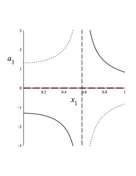
Figure 1: the graph of (5.3)

Consider case 2. Take a path $c:I\rightarrow\Lambda^{2}_{-}S^{4}$ given by

$$c(t)=\left({}^{t}\!(1,0,0,0,0),{}^{t}\!(a_{1}(t),a_{2}(t),a_{3}(t))\right).$$

We may assume that $a_{2}>0,a_{3}=0$ so that $c(t)$ is transverse to the ${\rm SO}(3)\times{\rm SO}(2)$-orbit. We find a path $c$ satisfying $\varphi_{\lambda}|_{({\rm SO}(3)\times{\rm SO}(2))\cdot{\rm Image}(c)}=0$, where $\varphi_{\lambda}$ is given by (3.1). Since $\dot{c}=\sum_{i=1}^{2}\dot{a}_{i}\frac{\partial}{\partial a_{i}}$, we have at $c(t)$

$$(\pi^{*}\omega_{i}(\tilde{E_{j}^{*}},\dot{c})) =0,$$

$$(b_{i}(\dot{c})) =\left(\dot{a}_{1},\dot{a}_{2},0\right),$$

$$\varphi_{\lambda}(\tilde{E_{1}^{*}},\tilde{E_{2}^{*}},\dot{c}) =2s_{\lambda}\dot{a}_{1},$$

$$\varphi_{\lambda}(\tilde{E_{p}^{*}},\tilde{E_{q}^{*}},\dot{c}) =0\qquad\mbox{for }\ (p,q)\neq(1,2),(2,1).$$

Thus the condition $\varphi_{\lambda}|_{({\rm SO}(3)\times{\rm SO}(2))\cdot{\rm Image}(c)}=0$ is equivalent to $a_{1}=C$ for $C\in\mathbb{R}$. Set $M_{C}={\rm SO}(3)\times{\rm SO}(2)\cdot\{({}^{t}\!(1,0,0,0,0),{}^{t}\!(C,r,0));r\in\mathbb{R}\}$. By (4.1) and (4.8), $M_{C}$ is explicitly described as

$$M_{C}= \left\{\left(\begin{array}[]{c}g_{11}\\ g_{21}\\ g_{31}\\ 0\\ 0\end{array}\right),\left(\begin{array}[]{ccc}g_{11}&g_{12}&-g_{13}\\ g_{21}&g_{22}&-g_{23}\\ -g_{31}&-g_{32}&g_{33}\\ \end{array}\right)\left(\begin{array}[]{ccc}1&0&0\\ 0&u&-v\\ 0&v&u\\ \end{array}\right)\left(\begin{array}[]{c}C\\ r\\ 0\\ \end{array}\right);\begin{array}[]{c}(g_{ij})\in{\rm SO}(3)\\ u^{2}+v^{2}=1\\ r\in\mathbb{R}\end{array}\right\}$$ (5.21)

$$= \left\{\left({}^{t}\!(x_{1},x_{2},x_{3},0,0),{}^{t}\!(a_{1},a_{2},a_{3})\right)\in S^{4}\times\mathbb{R}^{3};a_{1}x_{1}+a_{2}x_{2}-a_{3}x_{3}=C\right\}.$$

Thus $M_{C}$ is canonically identified with $\{(v,w)\in S^{2}\times\mathbb{R}^{3};\langle v,w\rangle=C\}$, which is homeomorphic to $\{(v,w)\in S^{2}\times\mathbb{R}^{3};\langle v,w\rangle=0\}=TS^{2}$ via $(v,w)\mapsto(v,w-Cv)$.

Remark 5.5.

Let $\Sigma^{2}\subset S^{4}$ be an oriented 2-submanifold. Let $L\rightarrow\Sigma$ be a line bundle over $\Sigma$ spanned by ${\rm vol}_{\Sigma}-*{\rm vol}_{\Sigma}$, where ${\rm vol}_{\Sigma}$ is a volume form of $\Sigma$ and $*$ is a Hodge star in $S^{4}$. Denote by $L^{\perp}$ the orthogonal complement bundle of $L$ in $\Lambda^{2}_{-}S^{4}$ and take a section $\eta$ of $L$ over $\Sigma$. By the argument in [13] and [12],

$$\eta+L^{\perp}=\left\{(x,\eta_{x}+\sigma)\in\Lambda^{2}_{-}S^{4}|_{\Sigma};x\in\Sigma,\sigma\in L^{\perp}_{x}\right\}$$

is coassociative if and only if $\Sigma$ is superminimal and $\eta\in\mathbb{R}({\rm vol}_{\Sigma}-*{\rm vol}_{\Sigma})$.

The submanifold $M_{C}$ is a special case of these examples. In fact, $\pi(M_{C})$ is a totally geodesic $S^{2}=\{{}^{t}\!(x_{1},x_{2},x_{3},0,0)\in S^{4}\}$ and define $\tau\in C^{\infty}(S^{2},\Lambda^{2}_{-}S^{4}|_{S^{2}})$ by

$$\tau_{x}=x_{1}(\omega_{1})_{x}+x_{2}(\omega_{2})_{x}-x_{3}(\omega_{3})_{x},$$

where $x={}^{t}\!(x_{1},x_{2},x_{3},0,0)\in S^{2}$. Note that $\tau$ is not the restriction of the tautological 2-form to $S^{2}$. We easily see that $M_{C}=C\tau+(\mathbb{R}\tau)^{\perp}$ and $\tau={\rm vol}_{S^{2}}-*{\rm vol}_{S^{2}}$ by the ${\rm SO}(3)$-invariance of $\tau$.

Consider case 3. Take a path $c:I\rightarrow\Lambda^{2}_{-}S^{4}$ given by

$$c(t)=\left({}^{t}\!(0,0,0,1,0),{}^{t}\!(a_{1}(t),a_{2}(t),a_{3}(t))\right).$$

We may assume that $a_{1}>0,a_{2}=a_{3}=0$ so that $c(t)$ is transverse to the ${\rm SO}(3)\times{\rm SO}(2)$-orbit. Since $\tilde{E_{1}^{*}}=a_{1}\frac{\partial}{\partial a_{2}}$, $\tilde{E_{2}^{*}}=-a_{1}\frac{\partial}{\partial a_{3}}$, $\tilde{E_{3}^{*}}=0,\tilde{E_{4}^{*}}=e_{4}$ at $c(t)$, we compute $\varphi_{\lambda}(\tilde{E_{1}^{*}},\tilde{E_{2}^{*}},\dot{c})=-a_{1}^{2}\dot{a}_{1}/s_{\lambda}^{3},$ which implies that $a_{1}$ is constant. Hence we cannot obtain a 4-submanifold.

5.3 Action of ${\rm U}(2)\subset{\rm SO}(4)\times\{1\}$

By Lemma 4.6, a ${\rm U}(2)$-orbit through $p_{0}=({}^{t}\!(x_{1},0,0,0,x_{5}),{}^{t}\!(0,0,a_{3}))$, where $x_{1}>0$, is 3-dimensional. At $p_{0}$, the stabilizer of the ${\rm U}(2)$-action is ${\rm U}(1)$. Thus a ${\rm U}(2)$-orbit through $p_{0}$ agrees with an ${\rm SU}(2)$-orbit through $p_{0}$. The case of ${\rm SU}(2)$ is considered in the next subsection.

5.4 Action of ${\rm SU}(2)\subset{\rm SO}(4)\times\{1\}$

We give a proof of Theorem 1.3. Recall the notation in Section 4.3 and 4.4. By Lemma 4.8, an ${\rm SU}(2)$-orbit through $({}^{t}\!(x_{1},0,0,0,x_{5}),{}^{t}\!(a_{1},a_{2},a_{3}))$ is 3-dimensional when $x_{5}\neq 0$. Take a path $c:I\rightarrow\Lambda^{2}_{-}S^{4}$ given by

$$c(t)=\left({}^{t}\!(x_{1}(t),0,0,0,x_{5}(t)),{}^{t}\!(a_{1}(t),a_{2}(t),a_{3}(t))\right),$$

where $x_{1}(t)>0$. We find a path $c$ satisfying $\varphi_{\lambda}|_{{\rm SU}(2)\cdot{\rm Image}(c)}=0$, where $\varphi_{\lambda}$ is given by (3.1). The condition $\varphi_{\lambda}(\tilde{E_{1}^{*}},\tilde{E_{2}^{*}},\tilde{E_{3}^{*}})=0$ is always satisfied. In fact, since the $G_{2}$-structure $\varphi_{\lambda}$ is preserved by the ${\rm SU}(2)$-action, we have $d(\varphi_{\lambda}(\tilde{E_{1}^{*}},\tilde{E_{2}^{*}},\tilde{E_{3}^{*}}))=0$ by Cartan’s formula. Since the action of ${\rm SU}(2)$ is not free, we have $\tilde{E_{1}^{*}}\wedge\tilde{E_{2}^{*}}\wedge\tilde{E_{3}^{*}}=0$ at some point. Thus we have $\varphi_{\lambda}(\tilde{E_{1}^{*}},\tilde{E_{2}^{*}},\tilde{E_{3}^{*}})=0$.

Lemma 5.6.

The condition $\varphi_{\lambda}|_{{\rm SU}(2)\cdot{\rm Image}(c)}=0$ is equivalent to

$$4\dot{a}_{i}\frac{1-x_{5}}{1+x_{5}}-a_{i}\frac{d}{dt}\left\{\log(\lambda+r^{2})+8\log(1+x_{5})\right\}=0\qquad\mbox{ for }i=1,2,3.$$ (5.22)

Proof.

Since $\dot{c}(t)=\left(-\dot{x}_{1}x_{5}+x_{1}\dot{x}_{5}\right)e_{4}+\sum_{j=1}^{3}\dot{a}_{j}\frac{\partial}{\partial a_{j}},$ we have

$$\left(\pi^{*}\omega_{i}(\tilde{E_{j}^{*}},\dot{c})\right) =\left(\begin{array}[]{ccc}0&-\dot{x}_{5}&0\\ -\dot{x}_{5}&0&0\\ 0&0&\dot{x}_{5}\\ \end{array}\right),$$

$$b_{j}(\dot{c}) =\dot{a_{j}}\qquad\mbox{ for }j=1,2,3.$$

Then we compute

$$\varphi_{\lambda}(\tilde{E_{1}^{*}},\tilde{E_{2}^{*}},\dot{c})|_{c}= \ 2s_{\lambda}\sum_{i=1}^{3}b_{i}\wedge\pi^{*}\omega_{i}(\tilde{E_{1}^{*}},\tilde{E_{2}^{*}},\dot{c})+\frac{1}{s_{\lambda}^{3}}b_{123}(\tilde{E_{1}^{*}},\tilde{E_{2}^{*}},\dot{c})$$

$$= 2s_{\lambda}\left(-2(1+x_{5})\dot{x}_{5}a_{3}+\dot{a}_{3}x_{1}^{2}\right)-\frac{(1+x_{5})^{2}a_{3}}{2s_{\lambda}^{3}}\frac{d(r^{2})}{dt}$$

$$= \frac{s_{\lambda}(1+x_{5})^{2}}{2}\left\{4\dot{a}_{3}\frac{1-x_{5}}{1+x_{5}}-a_{3}\frac{d}{dt}\left(\log(\lambda+r^{2})+8\log(1+x_{5})\right)\right\}.$$

We compute $\varphi_{\lambda}(E_{i}^{*},E_{i+1}^{*},\dot{c})|_{c}$ in the same way and we see the lemma. ∎

By (5.22), we have $\frac{d}{dt}{}^{t}\!\left(a_{1}(t),a_{2}(t),a_{3}(t)\right)=f(t){}^{t}\!\left(a_{1}(t),a_{2}(t),a_{3}(t)\right)$ for some function $f(t)$. The solution is given by ${}^{t}\!\left(a_{1}(t),a_{2}(t),a_{3}(t)\right)=\exp(\int^{t}f(s)ds)v$ for some $v\in\mathbb{R}^{3}$. Thus we may assume that ${}^{t}\!\left(a_{1}(t),a_{2}(t),a_{3}(t)\right)=r(t)v$ for a smooth function $r:I\rightarrow\mathbb{R}_{\geq 0}$ and $v\in S^{2}\subset\mathbb{R}^{3}$. Then (5.22) is solved explicitly as

$$F(r,x_{5})=C$$ (5.23)

for $C\in\mathbb{R}$, where $F:[0,\infty)\times[-1,1]\rightarrow\mathbb{R}$ is defined by

$$F(r,x_{5})=(1-3x_{5})(\lambda+r^{2})^{1/8}\sqrt{r}+\int^{\sqrt{r}}_{0}\frac{2\lambda}{(\lambda+x^{4})^{7/8}}dx.$$ (5.24)

This solution is obtained by Maple 16 [17]. Though the definition of $c$ implies that the domain of $F$ is $[0,\infty)\times(-1,1)$, $F$ extends to a map $[0,\infty)\times[-1,1]\rightarrow\mathbb{R}$ as in Remark 5.1. Thus we obtain the coassociative submanifold

$$M_{C,v}:={\rm SU}(2)\cdot\left\{\left({}^{t}\!(\sqrt{1-x_{5}^{2}},0,0,0,x_{5}),rv\right);F(r,x_{5})=C,r\geq 0,-1\leq x_{5}\leq 1\right\},$$

where $C\in\mathbb{R}$ and $v\in S^{2}\subset\mathbb{R}^{3}$. We study the topology of $M_{C,v}$ now.

Lemma 5.7.

The coassociative submanifold $M_{C}$ is homeomorphic to

$$\left\{\begin{array}[]{ll}\mathbb{R}^{4}&\qquad\mbox{for }\ C>0,\\ S^{4}\sqcup(S^{3}\times\mathbb{R}_{>0})&\qquad\mbox{for }\ C=0,\\ \mathcal{O}_{\mathbb{C}P^{1}}(-1)&\qquad\mbox{for }\ C<0,\end{array}\right.$$

where $S^{4}$ is the zero section of $\Lambda^{2}_{-}S^{4}$ and $\mathcal{O}_{\mathbb{C}P^{1}}(-1)$ is the tautological line bundle over $\mathbb{C}P^{1}\cong S^{2}$.

Proof.

Since we have

$$\frac{\partial F}{\partial x_{5}} =-3(\lambda+r^{2})^{1/8}\sqrt{r},$$

$$\frac{\partial F}{\partial r} =4^{-1}r^{-1/2}(\lambda+r^{2})^{-7/8}\left\{(1-3x_{5})(3r^{2}+2\lambda)+4\lambda\right\},$$

$F(r,\cdot)$ is monotonically decreasing on $[-1,1]$ for a fixed $r>0$ and $F(\cdot,-1)$ (resp. $F(\cdot,1)$) is monotonically increasing (resp. decreasing) on $\mathbb{R}_{\geq 0}$. We compute

$$F(0,\cdot)=0,\qquad\lim_{r\to\infty}F(r,\mp 1)=\pm\infty.$$

Thus for any $C>0$ (resp. $C<0$), there exists a unique $\alpha_{C}>0$ (resp. $\beta_{C}>0$) such that $C=F(\alpha_{C},-1)$ (resp. $C=F(\beta_{C},1)$).

Now, define a function $f_{C}:\mathbb{R}_{>0}\rightarrow\mathbb{R}$ by

$$f_{C}(r)=r^{-1/2}(\lambda+r^{2})^{-1/8}\left(C-\int^{\sqrt{r}}_{0}\frac{2\lambda}{(\lambda+x^{4})^{7/8}}dx\right).$$

Note that $F(x_{5},t)=C$ is equivalent to $1-3x_{5}=f_{C}(r)$. Since $-1\leq x_{5}\leq 1$, we may find the condition on $a_{1}$ so that $-2\leq f_{C}(r)\leq 4$.

Lemma 5.8.

When $C>0$, $f_{C}(r)>-2$ holds for any $r>0$ and $f_{C}(r)\leq 4$ is equivalent to $r\geq\alpha_{C}$. When $C<0$, $f_{C}(r)<4$ holds for any $r>0$ and $f_{C}(r)\geq-2$ is equivalent to $r\geq\beta_{C}$. When $C=0$, $-2<f_{C}(r)<4$ holds for any $r>0$.

Proof.

Suppose that $C>0$. Then $f_{C}(r)>-2$ is equivalent to $C>F(r,1)$, which holds for any $r>0$ since $F(r,1)<0$. The condition that $f_{C}(r)\leq 4$ is equivalent to $C=F(\alpha_{C},-1)\leq F(r,-1)$. Since $F(\cdot,-1)$ is monotonically increasing, this is equivalent to $r\geq\alpha_{C}$. We can prove similarly when $C\leq 0$. ∎

Remark 5.9.

Set $\Gamma(C)=\{(x_{5},r)\in[-1,1]\times[0,\infty);F(x_{5},r)=C\}.$ By Lemma 5.8, we have homeomorphisms $[\alpha_{C},\infty)\cong\Gamma(C)$ when $C>0$, $[\beta_{C},\infty)\cong\Gamma(C)$ when $C<0$, and $(0,\infty)\cong\Gamma(0)\cap\{r\neq 0\}$ via $r\mapsto((1-f_{C}(r))/3,r)$. Note that $\Gamma(C)\cap\{x_{5}=1\}=\emptyset$ when $C>0$, $\Gamma(C)\cap\{x_{5}=-1\}=\emptyset$ when $C<0$, and $\Gamma(0)\cap\{r\neq 0\}\cap\{x_{5}=\pm 1\}=\emptyset$.

Hence we see that

$$M_{0,v}\cap\{r>0\}=\left\{\left(\left(\begin{array}[]{c}\sqrt{1-x_{5}^{2}}a\\ \sqrt{1-x_{5}^{2}}b\\ x_{5}\end{array}\right),rv\right)\in\mathbb{C}^{2}\oplus\mathbb{R}\oplus\mathbb{R}^{3};\begin{array}[]{c}-1<x_{5}=\frac{1-f_{C}(r)}{3}<1,\\ r>0,\\ a,b\in\mathbb{C},\\ |a|^{2}+|b|^{2}=1\end{array}\right\},$$

which is homeomorphic to $S^{3}\times\mathbb{R}_{>0}$.

When $C\neq 0$, $M_{C,v}$ intersects with $\Lambda^{2}_{-}S^{4}|_{{}^{t}\!(0,0,0,0,\pm 1)}$. To study the topology of $M_{C,v}$, we use the stereographic local coordinates.

First, suppose that $\underline{C>0}$. By Remark 5.9, $M_{C,v}$ does not intersect with $\Lambda^{2}_{-}S^{4}|_{{}^{t}\!(0,0,0,0,1)}$. Take the stereographic local coordinates of $\Phi:S^{4}-\{x_{5}=1\}\rightarrow\mathbb{R}^{4}$ given by

$$\Phi(x_{1},\cdots,x_{5}) =\frac{\left(x_{1},x_{2},x_{3},-x_{4}\right)}{1-x_{5}},$$

$$\Phi^{-1}(y_{1},\cdots,y_{4}) =\frac{\left(2y_{1},2y_{2},2y_{3},-2y_{4},-1+|y|^{2}\right)}{1+|y|^{2}},$$

where $|y|^{2}=\Sigma_{i=1}^{4}y_{i}^{2}$. The standard metric on $S^{4}$ is given by $4\sum_{j=1}^{4}dy_{j}^{2}/(1+|y|^{2})^{2},$ and hence we see that $\left\{2dy_{i}/(1+|y|^{2})\right\}_{i=1,\cdots,4}$ is a local oriented orthonormal coframe. The trivialization $4(1+|y|^{2})^{-2}\{dy_{12}-dy_{34},dy_{13}-dy_{42},dy_{14}-dy_{23}\}$ of $\Lambda^{2}_{-}S^{4}$ induces the local fiber coordinates $(\alpha_{1},\alpha_{2},\alpha_{3})$. Setting $\zeta_{1}=y_{1}+iy_{2},\zeta_{2}=y_{3}+iy_{4}$, the action of ${\rm SU}(2)$ is described as

$$\left(\begin{array}[]{cc}a&-\overline{b}\\ b&\overline{a}\end{array}\right)\cdot({}^{t}\!(\zeta_{1},\zeta_{2}),{}^{t}\!(\alpha_{1},\alpha_{2},\alpha_{3}))=({}^{t}\!(a\zeta_{1}-\overline{b}\overline{\zeta_{2}},\overline{\beta}\overline{\zeta_{1}}+\alpha\zeta_{2}),{}^{t}\!(\alpha_{1},\alpha_{2},\alpha_{3})),$$

where $a,b\in\mathbb{C}$ such that $|a|^{2}+|b|^{2}=1$. Then we obtain

$$M_{C,v}=\left\{\left({}^{t}\!\left(y_{1}a,y_{1}b\right),rv^{\prime}\right)\in\mathbb{C}^{2}\oplus\mathbb{R}^{3};\begin{array}[]{c}r\in[\alpha_{C},\infty),y_{1}=\sqrt{\frac{6}{f_{C}(r)+2}-1},\\ a,b\in\mathbb{C},|a|^{2}+|b|^{2}=1\end{array}\right\},$$

where $v^{\prime}\in S^{2}$ is a corresponding element to $v$ under the change of local coordinates. Then it follows that $M_{C,v}$ is homeomorphic to $(S^{3}\times[\alpha_{C},\infty))/(S^{3}\times\{\alpha_{C}\})\cong\mathbb{R}^{4}$.

Next, suppose that $\underline{C<0}$. By Remark 5.9, $M_{C,v}$ does not intersect with $\Lambda^{2}_{-}S^{4}|_{{}^{t}\!(0,0,0,0,-1)}$. Take the stereographic local coordinates of $\Psi:S^{4}-\{x_{5}=-1\}\rightarrow\mathbb{R}^{4}$ given by

$$\Psi(x_{1},\cdots,x_{5}) =\frac{\left(x_{1},x_{2},x_{3},x_{4}\right)}{1+x_{5}},$$

$$\Psi^{-1}(u_{1},\cdots,u_{4}) =\frac{\left(2u_{1},2u_{2},2u_{3},2u_{4},1-|u|^{2}\right)}{1+|u|^{2}},$$

where $|u|^{2}=\Sigma_{i=1}^{4}u_{i}^{2}$. The standard metric on $S^{4}$ is given by $4\sum_{j=1}^{4}du_{j}^{2}/(1+|u|^{2})^{2},$ and hence we see that $\left\{2du_{i}/(1+|u|^{2})\right\}_{i=1,\cdots,4}$ is a local oriented orthonormal coframe. The trivialization $4(1+|u|^{2})^{-2}\{du_{12}-du_{34},du_{13}-du_{42},du_{14}-du_{23}\}$ of $\Lambda^{2}_{-}S^{4}$ induces the local fiber coordinates $(\underline{\alpha_{1}},\underline{\alpha_{2}},\underline{\alpha_{3}})$. Setting $\underline{\zeta_{1}}=u_{1}+iu_{2},\underline{\zeta_{2}}=u_{3}+iu_{4}$, the action of ${\rm SU}(2)$ is described as

$$g\cdot({}^{t}\!(\underline{\zeta_{1}},\underline{\zeta_{2}}),{}^{t}\!(\underline{\alpha_{1}},\underline{\alpha_{2}},\underline{\alpha_{3}}))=(g{}^{t}\!(\underline{\zeta_{1}},\underline{\zeta_{2}}),\varpi(g){}^{t}\!(\underline{\alpha_{1}},\underline{\alpha_{2}},\underline{\alpha_{3}})),$$ (5.25)

where $g\in{\rm SU}(2)$ and $\varpi:{\rm SU}(2)\rightarrow{\rm SO}(3)$ is a double covering given by (4.35). Then we obtain

$$M_{C,v}=\left\{\left(g{}^{t}\!(u_{1},0\right),r\varpi(g)v^{\prime})\in\mathbb{C}^{2}\oplus\mathbb{R}^{3};\begin{array}[]{c}r\in[\beta_{C},\infty),u_{1}=\sqrt{\frac{6}{4-f_{C}(r)}-1},\\ g\in{\rm SU}(2)\end{array}\right\},$$ (5.28)

where $v^{\prime}\in S^{2}$ is a corresponding element to $v$ under the change of local coordinates.

Note that the topology of $M_{C,v}$ is independent of $v$. In fact, fix $v_{0}\in S^{2}$ and let $v_{0}^{\prime}$ be a corresponding element to $v_{0}$ under the change of local coordinates.

For any $v\in S^{2}$, there exists $g_{0}\in{\rm SU}(2)$ such that $v^{\prime}=\varpi(g_{0})v_{0}^{\prime}$. Then $M_{C,v}\cong M_{C,v_{0}}$ via $(g{}^{t}\!(u_{1},0),r\varpi(g)v^{\prime})\mapsto(gg_{0}{}^{t}\!(u_{1},0),r\varpi(g)v^{\prime}).$ Thus we only have to consider the case $v_{0}^{\prime}={}^{t}\!(1,0,0)$. Setting $v_{0}^{\prime}={}^{t}\!(1,0,0)$ in (5.28), we obtain

$$\left\{\left({}^{t}\!(u_{1}a,u_{1}b\right),r{}^{t}\!(|a|^{2}-|b|^{2},2{\rm Im}(a\overline{b}),2{\rm Re}(a\overline{b}));\begin{array}[]{c}r\in[\beta_{C},\infty),u_{1}=\sqrt{\frac{6}{4-f_{C}(r)}-1},\\ a,b\in\mathbb{C},|a|^{2}+|b|^{2}=1\end{array}\right\},$$

which is homeomorphic to

$$\left\{(v,[w,r])\in S^{2}\times(S^{3}\times[\beta_{C},\infty))/(S^{3}\times\{\beta_{C}\});w\in p^{-1}(v)\right\},$$

where $p:S^{3}\rightarrow\mathbb{C}P^{1}=S^{2}$ is the Hopf fibration. This is the tautological line bundle $\mathcal{O}_{\mathbb{C}P^{1}}(-1)$ over $\mathbb{C}P^{1}$. ∎

Remark 5.10.

When $\lambda=0$, (5.23) is given by

$$(1-3x_{5})r^{3/4}=C.$$ (5.29)

We exhibit the graph of (5.29). The solid curve indicates the case $C>0$, the dashed curve indicates the case $C=0$ and the dotted curve indicates the case $C<0$. We see that the solution (5.23) is asymptotic to this graph as $\lambda\rightarrow 0$. The vertical line gives a coassociative cone in $\Lambda^{2}_{-}S^{4}-\{\mbox{zero section}\}\cong\mathbb{C}P^{3}\times\mathbb{R}_{>0}$, which corresponds to a Lagrangian submanifold in the nearly Kähler $\mathbb{C}P^{3}$.

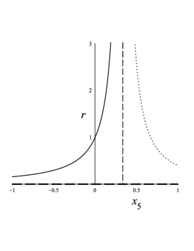
Figure 2: the graph of (5.29)

5.5 ${\rm SO}(3)={\rm SO}(3)\times\{I_{2}\}$-action

We give a proof of Theorem 1.4. Recall the notation in Section 4.5. By Lemma 4.9, an ${\rm SO}(3)$-orbit through $({}^{t}\!(x_{1},0,0,x_{4},x_{5}),{}^{t}\!(a_{1},a_{2},a_{3}))$ is 3-dimensional when $x_{1}>0,(a_{2},a_{3})\neq 0$. Take a path $c:I\rightarrow\Lambda^{2}_{-}S^{4}$ given by

$$c(t)=\left({}^{t}\!(x_{1}(t),0,0,x_{4}(t),x_{5}(t)),{}^{t}\!(a_{1}(t),a_{2}(t),0)\right),$$

where $x_{1}(t)>0,a_{2}(t)>0$. We assume that $a_{3}=0$ so that $c(t)$ is transverse to the ${\rm SO}(3)$-orbits. We find a path $c$ satisfying $\varphi_{\lambda}|_{{\rm SO}(3)\cdot{\rm Image}(c)}=0$, where $\varphi_{\lambda}$ is given by (3.1). We see that $\varphi_{\lambda}(\tilde{E_{1}^{*}},\tilde{E_{2}^{*}},\tilde{E_{3}^{*}})=0$ as in Section 5.4.

Lemma 5.11.

The condition $\varphi_{\lambda}|_{{\rm SO}(3)\cdot{\rm Image}(c)}=0$ is equivalent to

$$4(2x_{1}\dot{x}_{1}a_{1}+\dot{a}_{1}x_{1}^{2})-(1-x_{1}^{2})a_{1}\frac{d}{dt}\log(\lambda+r^{2}) =0,$$ (5.30)

$$4x_{1}\dot{x}_{1}-\frac{d}{dt}\log(\lambda+r^{2})+\frac{x_{1}^{2}}{1-x_{5}}\left(4\dot{x}_{5}+\frac{d}{dt}\log(\lambda+r^{2})\right) =0,$$ (5.31)

$$4\dot{x}_{4}+\frac{x_{4}}{1-x_{5}}\left(4\dot{x}_{5}+\frac{d}{dt}\log(\lambda+r^{2})\right) =0,$$ (5.32)

where $r^{2}=a_{1}^{2}+a_{2}^{2}$.

Proof.

Since $\dot{c}=\frac{-\dot{x}_{1}x_{4}+x_{1}\dot{x}_{4}}{\sqrt{1-x_{5}^{2}}}e_{3}+\frac{\dot{x}_{5}}{\sqrt{1-x_{5}^{2}}}e_{4}+\dot{a}_{1}\frac{\partial}{\partial a_{1}}+\dot{a}_{2}\frac{\partial}{\partial a_{2}},$ we have

$$(\pi^{*}\omega_{i}(\tilde{E_{j}^{*}},\dot{c}))=\left(\begin{array}[]{ccc}0&0&0\\ x_{1}\dot{x}_{4}+\frac{x_{1}x_{4}\dot{x}_{5}}{1-x_{5}}&x_{1}\dot{x}_{1}+\frac{x_{1}^{2}\dot{x}_{5}}{1-x_{5}}&0\\ x_{1}\dot{x}_{1}+\frac{x_{1}^{2}\dot{x}_{5}}{1-x_{5}}&-x_{1}\dot{x}_{4}-\frac{x_{1}x_{4}\dot{x}_{5}}{1-x_{5}}&0\end{array}\right),(b_{i}(\dot{c}))=\left(\begin{array}[]{c}\dot{a}_{1}\\ \dot{a}_{2}\\ \frac{-\dot{x}_{1}x_{4}+x_{1}\dot{x}_{4}}{1-x_{5}}a_{2}\end{array}\right).$$

Then we compute

$$\sum_{i=1}^{3}b_{i}\wedge\pi^{*}\omega_{i}(\tilde{E_{1}^{*}},\tilde{E_{2}^{*}},\dot{c})= 2x_{1}a_{1}\left\{-\frac{x_{1}x_{4}\dot{x}_{4}}{1-x_{5}}+\left(1-\frac{x_{1}^{2}+x_{4}^{2}}{1-x_{5}}\right)\frac{x_{1}\dot{x}_{5}}{1-x_{5}}\right.$$

$$\left.+\left(1-\frac{x_{1}^{2}}{1-x_{5}}\right)\dot{x}_{1}\right\}+\dot{a}_{1}x_{1}^{2},$$

$$b_{123}(\tilde{E_{1}^{*}},\tilde{E_{2}^{*}},\dot{c})= -\left\{\left(1-\frac{x_{1}^{2}}{1-x_{5}}\right)^{2}+\frac{x_{1}^{2}x_{4}^{2}}{(1-x_{5})^{2}}\right\}a_{1}(a_{1}\dot{a}_{1}+a_{2}\dot{a}_{2})$$

Since $x_{1}^{2}+x_{4}^{2}+x_{5}^{2}=1,x_{1}\dot{x}_{1}+x_{4}\dot{x}_{4}+x_{5}\dot{x}_{5}=0$, it follows that

$$\sum_{i=1}^{3}b_{i}\wedge\pi^{*}\omega_{i}(\tilde{E_{1}^{*}},\tilde{E_{2}^{*}},\dot{c})=2x_{1}\dot{x}_{1}a_{1}+\dot{a}_{1}x_{1}^{2},\qquad b_{123}(\tilde{E_{1}^{*}},\tilde{E_{2}^{*}},\dot{c})=-\frac{(1-x_{1}^{2})a_{1}}{2}\frac{d(r^{2})}{dt},$$

which implies (5.30). In the same way, we compute

$$\sum_{i=1}^{3}b_{i}\wedge\pi^{*}\omega_{i}(\tilde{E_{1}^{*}},\tilde{E_{3}^{*}},\dot{c}) =a_{2}\left(x_{1}\dot{x}_{1}+\frac{x_{1}^{2}\dot{x}_{5}}{1-x_{5}}\right),$$

$$b_{123}(\tilde{E_{1}^{*}},\tilde{E_{3}^{*}},\dot{c}) =\left(-1+\frac{x_{1}^{2}}{1-x_{5}}\right)\frac{a_{2}}{2}\frac{d(r^{2})}{dt},$$

$$\sum_{i=1}^{3}b_{i}\wedge\pi^{*}\omega_{i}(\tilde{E_{2}^{*}},\tilde{E_{3}^{*}},\dot{c}) =-a_{2}\left(x_{1}\dot{x}_{4}+\frac{x_{1}x_{4}\dot{x}_{5}}{1-x_{5}}\right),$$

$$b_{123}(\tilde{E_{2}^{*}},\tilde{E_{3}^{*}},\dot{c}) =-\frac{x_{1}x_{4}a_{2}}{2(1-x_{5})}\frac{d(r^{2})}{dt},$$

and obtain (5.31) and (5.32). ∎

Next, we solve (5.30), (5.31), (5.32). Calculating $(\ref{SO3 eq2})+x_{4}\cdot(\ref{SO3 eq3})$, we have

$$4\dot{x}_{5}+x_{5}\frac{d}{dt}\log(\lambda+r^{2})=0.$$ (5.33)

Substitution of (5.33) into (5.32) gives

$$4\dot{x}_{4}+x_{4}\frac{d}{dt}\log(\lambda+r^{2})=0.$$ (5.34)

From (5.33) and (5.34), we have

$$(1-x_{1}^{2})\frac{d}{dt}\log(\lambda+r^{2}) =(x_{4}^{2}+x_{5}^{2})\frac{d}{dt}\log(\lambda+r^{2})$$

$$=-4(x_{4}\dot{x}_{4}+x_{5}\dot{x}_{5})$$

$$=4x_{1}\dot{x}_{1}.$$

which implies that (5.30) is equivalent to

$$x_{1}\frac{d}{dt}(a_{1}x_{1})=0.$$ (5.35)

Equations (5.33), (5.34), (5.35) are solved easily and we obtain

$$x_{4}^{4}(\lambda+r^{2})=C,\qquad x_{5}^{4}(\lambda+r^{2})=D,\qquad a_{1}x_{1}=E$$

for $C,D\geq 0,E\in\mathbb{R}$. Thus

$$M_{C,D,E}={\rm SO}(3)\cdot\left\{({}^{t}\!(x_{1},0,0,x_{4},x_{5}),{}^{t}\!(a_{1},a_{2},0));\begin{array}[]{c}x_{4}^{4}(\lambda+r^{2})=C,\\ x_{5}^{4}(\lambda+r^{2})=D,\\ a_{1}x_{1}=E\end{array}\right\}$$

is a coassociative submanifold for $C,D\geq 0,E\in\mathbb{R}$.

Next, we consider the topology of $M_{C,D,E}$.

Lemma 5.12.

Set $N=(\mathbb{R}_{\geq 0}\times{\rm SO}(3))/(\{0\}\times{\rm SO}(3))$, which is the cone over ${\rm SO}(3)$ with the apex. Then the topology of $M_{C,D,E}$ is given by the following.

condition	topology of $M_{C,D,E}$
$C>0,D>0,E=0,\sqrt{C}+\sqrt{D}\neq\sqrt{\lambda}$	$TS^{2}\sqcup TS^{2}\sqcup TS^{2}\sqcup TS^{2}$
$C>0,D>0,E=0,\sqrt{C}+\sqrt{D}=\sqrt{\lambda}$	$N\sqcup N\sqcup N\sqcup N$
$C>0,D>0,E\neq 0$	$TS^{2}\sqcup TS^{2}\sqcup TS^{2}\sqcup TS^{2}$
$C=0,D=0$	$TS^{2}$
$C>0,D=0,E=0,\sqrt{C}\neq\sqrt{\lambda}$	$TS^{2}\sqcup TS^{2}$
$C>0,D=0,E=0,\sqrt{C}=\sqrt{\lambda}$	$N\sqcup N$
$C>0,D=0,E\neq 0$	$TS^{2}\sqcup TS^{2}$
$C=0,D>0,E=0,\sqrt{D}\neq\sqrt{\lambda}$	$TS^{2}\sqcup TS^{2}$
$C=0,D>0,E=0,\sqrt{D}=\sqrt{\lambda}$	$N\sqcup N$
$C=0,D>0,E\neq 0$	$TS^{2}\sqcup TS^{2}$

Lemma 5.13.

For any convergent sequence $\{(C_{j},D_{j})\}\subset(\mathbb{R}_{>0})^{2}$ satisfying $\sqrt{C_{j}}+\sqrt{D_{j}}<\sqrt{\lambda}$ for any $j$ (or $\sqrt{C_{j}}+\sqrt{D_{j}}>\sqrt{\lambda}$ for any $j$) and $\sqrt{C_{\infty}}+\sqrt{D_{\infty}}=\sqrt{\lambda}$, where $C_{\infty}=\lim_{j\to\infty}C_{j},D_{\infty}=\lim_{j\to\infty}D_{j}$, $M_{C_{j},D_{j},0}$ converges to $M_{C_{\infty},D_{\infty},0}$ in the sense of currents.

Similarly, for any convergent sequence $\{C_{j}\}\subset\mathbb{R}_{>0}$ satisfying $\sqrt{C_{j}}<\sqrt{\lambda}$ for any $j$ (or $\sqrt{C_{j}}>\sqrt{\lambda}$ for any $j$) and $\sqrt{C_{\infty}}=\sqrt{\lambda}$, where $C_{\infty}=\lim_{j\to\infty}C_{j}$, $M_{C_{j},0,0}$ converges to $M_{C_{\infty},0,0}$ and $M_{0,C_{j},0}$ converges to $M_{0,C_{\infty},0}$ in the sense of currents.

Proof of Lemma 5.12.

First, suppose that $M_{C,D,E}$ does not intersect with $\Lambda^{2}_{-}S^{4}|_{{}^{t}\!(0,0,0,0,\pm 1)}$. Then by (4.1) we see that

$$M_{C,D,E}=\left\{\left(\left(\begin{array}[]{c}g_{11}x_{1}\\ g_{21}x_{1}\\ g_{31}x_{1}\\ x_{4}\\ x_{5}\end{array}\right),\left(\begin{array}[]{c}a_{1}g_{11}+a_{2}g_{12}\\ a_{1}g_{21}+a_{2}g_{22}\\ -a_{1}g_{31}-a_{2}g_{32}\end{array}\right)\right);\begin{array}[]{c}x_{4}^{4}(\lambda+r^{2})=C,\\ x_{5}^{4}(\lambda+r^{2})=D,\\ a_{1}x_{1}=E,\\ (g_{ij})\in{\rm SO}(3)\end{array}\right\}$$

$$=\left\{\left(\left(\begin{array}[]{c}x_{1}\\ x_{2}\\ x_{3}\\ x_{4}\\ x_{5}\end{array}\right),\left(\begin{array}[]{c}a_{1}\\ a_{2}\\ a_{3}\end{array}\right)\right)\in S^{4}\times\mathbb{R}^{3};\begin{array}[]{c}x_{4}^{4}(\lambda+r^{2})=C,\\ x_{5}^{4}(\lambda+r^{2})=D,\\ (r^{2}=\sum_{i=1}^{3}a_{i}^{2})\\ a_{1}x_{1}+a_{2}x_{2}-a_{3}x_{3}=E\\ \end{array}\right\}.$$

We study the topology of $M_{C,D,E}$ in the following cases:

1. $C>0,D>0$,

   1. $E=0,\sqrt{C}+\sqrt{D}<\sqrt{\lambda}$,

   2. $E=0,\sqrt{C}+\sqrt{D}>\sqrt{\lambda}$,

   3. $E=0,\sqrt{C}+\sqrt{D}=\sqrt{\lambda}$,

   4. $E\neq 0$,

2. $C=0,D=0$,

3. $C>0,D=0$,

4. $C=0,D>0$.

Consider case 1. Then $M_{C,D,E}$ does not intersect with $\Lambda^{2}_{-}S^{4}|_{{}^{t}\!(0,0,0,0,\pm 1)}$. Set

$$M_{C,D,E}^{\pm,+} =M_{C,D,E}\cap\{\pm x_{4}>0\}\cap\{x_{5}>0\},$$

$$M_{C,D,E}^{\pm,-} =M_{C,D,E}\cap\{\pm x_{4}>0\}\cap\{x_{5}<0\}.$$

Each $M_{C,D,E}^{\pm,\pm}$ is a connected component of $M_{C,D,E}$ and is homeomorphic to

$$N_{C,D,E}=\left\{(v,w)\in\mathbb{R}^{3}\times\mathbb{R}^{3};\langle v,w\rangle=E,(1-|v|^{2})\sqrt{\lambda+|w|^{2}}=\sqrt{C}+\sqrt{D}\right\}.$$ (5.36)

We only have to consider the topology of $N_{C,D,E}$.

Consider case 1-(a). We have $|v|^{2}=1-(\sqrt{C}+\sqrt{D})/\sqrt{\lambda+|w|^{2}}\geq 1-(\sqrt{C}+\sqrt{D})/\sqrt{\lambda}>0$. Hence there is an homeomorphism $N_{C,D,0}\rightarrow\{(v,w)\in S^{2}\times\mathbb{R}^{3};\langle v,w\rangle=0\}=TS^{2}$ via $(v,w)\mapsto(v/|v|,w)$.

Consider case 1-(b). We have $|w|^{2}=(\sqrt{C}+\sqrt{D})^{2}/(1-|v|^{2})^{2}-\lambda\geq(\sqrt{C}+\sqrt{D})^{2}-\lambda>0$. Hence there is an homeomorphism $N_{C,D,0}\rightarrow\{(w,v)\in S^{2}\times\mathbb{R}^{3};\langle w,v\rangle=0,|v|<1\}\cong TS^{2}$ via $(v,w)\mapsto(w/|w|,v)$.

Consider case 1-(c). A map $N=(\mathbb{R}_{\geq 0}\times{\rm SO}(3))/(\{0\}\times{\rm SO}(3))\rightarrow N_{C,D,0}$ defined by $[(r,(g_{1},g_{2},g_{3})]\mapsto(f(r)g_{1},rg_{2})$, where $g_{i}\in\mathbb{R}^{3}$, $\langle g_{i},g_{j}\rangle=\delta_{ij}$, and $f(r)=\sqrt{1-(\sqrt{C}+\sqrt{D})/\sqrt{\lambda+r^{2}}}$, gives a homeomorphism.

Consider case 1-(d). Since $N_{C,D,E}\cong N_{C,D,-E}$ via $(v,w)\mapsto(v,-w)$, we may assume that $E>0$. Since $E\neq 0$, we have $v,w\neq 0$ for any $(v,w)\in N_{C,D,E}.$ Define $c_{0}\in\mathbb{R}$ and a function $f:(c_{0},\infty)\rightarrow(f(c_{0}),1)$ by

$$c_{0} =\left\{\begin{array}[]{ll}0&\qquad\mbox{when }\ (\sqrt{C}+\sqrt{D})^{2}-\lambda\leq 0,\\ \sqrt{(\sqrt{C}+\sqrt{D})^{2}-\lambda}&\qquad\mbox{when }\ (\sqrt{C}+\sqrt{D})^{2}-\lambda\geq 0\end{array}\right.,$$

$$f(r) =\sqrt{1-\frac{\sqrt{C}+\sqrt{D}}{\sqrt{\lambda+r^{2}}}}.$$

Then $f$ is bijective and monotonically increasing. Note that for $(v,w)\in N_{C,D,E}$, we have $f(|w|)=|v|$. Since $rf(r):(c_{0},\infty)\rightarrow(0,\infty)$ is bijective and monotonically increasing, there exists a unique $d_{0}>c_{0}>0$ such that $d_{0}f(d_{0})=E$. Now define a function $g:[d_{0},\infty)\rightarrow[0,\infty)$ by $g(r)=\sqrt{r^{2}-(E^{2}/f(r)^{2})}$. Note that for $(v,w)\in N_{C,D,E}$, we have $|w-(Ev/|v|^{2})|=g(|w|)$.

Define a map $\Phi:N_{C,D,E}\rightarrow\{(v^{\prime},w^{\prime})\in S^{2}\times\mathbb{R}^{3};\langle v,w\rangle=0\}=TS^{2}$ by $\Phi(v,w)=(v/|v|,w-(Ev/|v|^{2}))$. Then $\Phi$ is a homeomorphism and the inverse map $\Phi^{-1}$ is given by $\Phi^{-1}(v^{\prime},w^{\prime})=(f(g^{-1}(|w^{\prime}|))v^{\prime},w^{\prime}+(Ev^{\prime}/f(g^{-1}(|w^{\prime}|))))$.

Consider case 2. By definition, we have $x_{4}=x_{5}=0$. Then

$$M_{0,0,E}=\left\{\left({}^{t}\!\left(x_{1},x_{2},x_{3},0,0\right),{}^{t}\!\left(a_{1},a_{2},a_{3}\right)\right)\in S^{4}\times\mathbb{R}^{3};a_{1}x_{1}+a_{2}x_{2}-a_{3}x_{3}=E\right\},$$

which is obtained in (5.21) and is homeomorphic to $TS^{2}$.

Consider case 3. By definition, we have $x_{5}=0$ and

$$M_{C,0,E}=\left\{\left({}^{t}\!\left(x_{1},x_{2},x_{3},x_{4},0\right),{}^{t}\!\left(a_{1},a_{2},a_{3}\right)\right)\in S^{4}\times\mathbb{R}^{3};\begin{array}[]{c}x_{4}^{4}(\lambda+r^{2})=C,\\ a_{1}x_{1}+a_{2}x_{2}-a_{3}x_{3}=E\end{array}\right\}.$$

Set $M_{C,0,E}^{\pm}=M_{C,0,E}\cap\{\pm x_{4}>0\}.$ Each $M_{C,0,E}^{\pm}$ is a connected component of $M_{C,0,E}$ and is homeomorphic to $N_{C,0,E}$ defined in (5.36).

Consider case 4. By (4.8), $\left(\begin{array}[]{cc}0&1\\ -1&0\end{array}\right)\in{\rm SO}(2)=\{I_{3}\}\times{\rm SO}(2)\subset{\rm SO}(5)$ gives a homeomorphism from $N_{0,D,E}$ to $N_{D,0,E}$. Hence this case is reduced to case 3. ∎

Proof of Lemma 5.13.

We only have to prove that $N_{C_{j},D_{j},0}$ converges to $N_{C_{\infty},D_{\infty},0}-\{(0,0)\}$ in the sense of currents. Note that sets differing only a set of measure zero are identified in the theory of currents.

Suppose that $\sqrt{C_{j}}+\sqrt{D_{j}}<\sqrt{\lambda}$ for any $j$. Then by the proof of Lemma 5.12, there is a homeomorphism $h_{C_{j},D_{j}}:N_{C_{j},D_{j},0}\rightarrow\{(v,w)\in S^{2}\times\mathbb{R}^{3};\langle v,w\rangle=0\}=TS^{2}$ via $(v,w)\mapsto(v/|v|,w)$. Note that $h_{C_{j},D_{j}}^{-1}$ is given by $(v^{\prime},w^{\prime})\mapsto(f_{C_{j},D_{j}}(|w^{\prime}|)v^{\prime},w^{\prime})$, where $f_{C_{j},D_{j}}(r)=\sqrt{1-(\sqrt{C_{j}}+\sqrt{D_{j}})/\sqrt{\lambda+r^{2}}}$.

On the other hand, $N_{C_{\infty},D_{\infty},0}-\{(0,0)\}$ is homeomorphic to $TS^{2}-\{0\}$ via $h_{C_{\infty},D_{\infty}}:(v,w)\mapsto(v/|v|,w)$ and $h_{C_{\infty},D_{\infty}}^{-1}$ is given by $(v^{\prime},w^{\prime})\mapsto(f_{C_{\infty},D_{\infty}}(|w^{\prime}|)v^{\prime},w^{\prime})$. Then we see that for any compactly supported 4-form $\alpha$ on $\mathbb{R}^{3}\times\mathbb{R}^{3}$

$$\int_{N_{C_{j},D_{j},0}}\alpha=\int_{TS^{2}-\{0\}}(h_{C_{j},D_{j}}^{-1})^{*}\alpha\rightarrow\int_{TS^{2}-\{0\}}(h_{C_{\infty},D_{\infty}}^{-1})^{*}\alpha=\int_{N_{C_{\infty},D_{\infty},0}-\{(0,0)\}}\alpha,$$

which implies that $N_{C_{j},D_{j},0}$ converges to $N_{C_{\infty},D_{\infty},0}-\{(0,0)\}$ in the sense of currents. We can prove the other cases similarly and obtain the statement. ∎

Remark 5.14.

Use the notation in [16]. By Lemma 5.12, $M_{C,D,E}$ is a coassociative submanifold with conical singularities when (i) $C>0,D>0,E=0,\sqrt{C}+\sqrt{D}=\sqrt{\lambda}$, (ii)$C>0,D=0,E=0,\sqrt{C}=\sqrt{\lambda}$, or (iii)$C=0,D>0,E=0,\sqrt{D}=\sqrt{\lambda}$. In each case, the tangent cone is modeled on $C(L)=\mathbb{R}_{>0}\times L$, where $L$ is given by

$$L=\left\{{}^{t}\!(0,z_{1},z_{2},z_{3})\in\mathbb{R}\oplus\mathbb{C}^{3};z_{1}^{2}+z_{2}^{2}+\overline{z}_{3}^{2}=0,|z_{1}|^{2}+|z_{2}|^{2}+|z_{3}|^{2}=1\right\}\cong{\rm SO}(3).$$

We calculate the rate at singular points as follows. For simplicity, we only consider the case of $M^{+}_{\lambda,0,0}$ which is singular at $p_{0}=\left({}^{t}\!(0,0,0,1,0),{}^{t}\!(0,0,0)\right)$.

Let $B(0,r)\subset\mathbb{R}^{4}$ be an open ball of radius $r$. Set $D=\{x_{4}>0\}\subset S^{4}$ and $k=2^{-1/2}\lambda^{-1/4}$. Define $\chi:B(0,1/k)\times\mathbb{R}^{3}\rightarrow D\times\mathbb{R}^{3}$ by

$$\left({}^{t}\!(u_{1},u_{2},u_{3},u_{4}),{}^{t}\!(a_{1},a_{2},a_{3})\right)\mapsto\left({}^{t}\!(-ku_{3},ku_{2},-ku_{1},\sqrt{1-k^{2}|u|^{2}},ku_{4}),\lambda^{1/4}{}^{t}\!(a_{1},a_{2},a_{3})\right),$$

where $|u|^{2}=\sum_{j=1}^{4}u_{j}^{2}$. Since $(d\chi)_{0}(\frac{\partial}{\partial u_{i}})_{0}=k(e_{i})_{p_{0}},(d\chi)_{0}(\frac{\partial}{\partial a_{i}})_{0}=\lambda^{1/4}(\frac{\partial}{\partial a_{i}})_{p_{0}}$, we see that $(d\chi)_{0}^{*}(\varphi_{\lambda})_{p_{0}}=\varphi_{0}$, where $\varphi_{0}$ is a 3-form on $\mathbb{R}^{7}$ given by (2.1). Note that

$$\chi^{-1}(M^{+}_{\lambda,0,0})=\left\{{}^{t}\!(u_{1},u_{2},u_{3},0,a_{1},a_{2},a_{3});\begin{array}[]{l}(1-k^{2}|u|^{2})^{2}\left(1+\sum_{j=1}^{3}a_{j}^{2}\right)=1,\\ -u_{3}a_{1}+u_{2}a_{2}-u_{1}a_{3}=0\end{array}\right\}.$$

Define $\Phi:\mathbb{R}_{>0}\times L\rightarrow\mathbb{R}^{7}$ by

$$\left(r,{}^{t}\!(0,x_{1}+iy_{1},x_{2}+iy_{2},x_{3}+iy_{3})\right)\mapsto{}^{t}\!\left(f(r)x_{1},f(r)x_{2},f(r)x_{3},0,ry_{3},ry_{2},-ry_{1}\right),$$

where $f(r)=2\lambda^{1/4}\sqrt{1-\sqrt{\frac{2}{2+r^{2}}}}$. This gives the diffeomorphism $\chi\circ\Phi:\mathbb{R}_{>0}\times L\rightarrow M^{+}_{\lambda,0,0}-\{p_{0}\}$. Since we see that $f(r)=\lambda^{1/4}r+O(r^{3})$ as $r\rightarrow 0$, we see that the rate at $p_{0}$ is equal to 3 in these coordinates.

5.6 Irreducible ${\rm SO}(3)$-action

We give a proof of Theorem 1.5. Recall the notation in Section 4.6. By Lemma 4.12, an ${\rm SO}(3)$-orbit through $({}^{t}\!(x_{1},0,0,0,x_{5}),{}^{t}\!(a_{1},a_{2},a_{3}))$ is 3-dimensional when

1. $-1/2<x_{5}<1/2$,

2. $x_{5}=1/2,(a_{1},a_{3})\neq 0$, or

3. $x_{5}=-1/2,(a_{2},a_{3})\neq 0$.

Consider case 1. Take a path $c:I\rightarrow\Lambda^{2}_{-}S^{4}$ given by

$$c(t)=\left({}^{t}\!(x_{1}(t),0,0,0,x_{5}(t)),{}^{t}\!(a_{1}(t),a_{2}(t),a_{3}(t))\right),$$

where $x_{1}(t)>0,|x_{5}(t)|<1/2$. We find a path $c$ satisfying $\varphi_{\lambda}|_{{\rm SO}(3)\cdot{\rm Image}(c)}=0$, where $\varphi_{\lambda}$ is given by (3.1). We see that $\varphi_{\lambda}(\tilde{E_{1}^{*}},\tilde{E_{2}^{*}},\tilde{E_{3}^{*}})=0$ as in Section 5.4.

Lemma 5.15.

The condition $\varphi_{\lambda}|_{{\rm SO}(3)\cdot{\rm Image}(c)}=0$ is equivalent to

$$4\left\{(2\sqrt{3}x_{1}+4x_{5}+1)\dot{x}_{5}+\sqrt{3}(2x_{5}-1)\dot{x}_{1}\right\}a_{1}+8x_{1}(-x_{1}+\sqrt{3}x_{5})\dot{a}_{1}$$

$$-(\sqrt{3}x_{1}+x_{5}+1)(1-2x_{5})a_{1}\frac{d}{dt}\log(\lambda+r^{2}) =0,$$ (5.37)

$$4\left\{(2\sqrt{3}x_{1}-4x_{5}-1)\dot{x}_{5}+\sqrt{3}(2x_{5}-1)\dot{x}_{1}\right\}a_{2}+8x_{1}(x_{1}+\sqrt{3}x_{5})\dot{a}_{2}$$

$$+(-\sqrt{3}x_{1}+x_{5}+1)(1-2x_{5})a_{2}\frac{d}{dt}\log(\lambda+r^{2}) =0,$$ (5.38)

$$4\left\{-(x_{5}+1)\dot{x}_{5}+3x_{1}\dot{x}_{1}\right\}a_{3}+2(x_{1}^{2}-3x_{5}^{2})\dot{a}_{3}$$

$$+(1+x_{5})(1-2x_{5})a_{3}\frac{d}{dt}\log(\lambda+r^{2}) =0,$$ (5.39)

where $r^{2}=\sum_{j=1}^{3}a_{j}^{2}$.

This lemma implies Theorem 1.5. In general, it is hard to solve the equations (5.37), (5.38), (5.39) explicitly.

Proof.

Since $\dot{c}=(-\dot{x}_{1}x_{5}+x_{1}\dot{x}_{5})e_{4}+\sum_{j=1}^{3}\dot{a}_{j}\frac{\partial}{\partial a_{j}},$ we have

$$(\pi^{*}\omega_{i}(\tilde{E_{j}^{*}},\dot{c})) =\left(\begin{array}[]{ccc}-\dot{x}_{5}+\sqrt{3}\dot{x}_{1}&0&0\\ 0&0&\dot{x}_{5}+\sqrt{3}\dot{x}_{1}\\ 0&-2\dot{x}_{5}&0\end{array}\right),$$

$$b_{j}(\dot{c}) =a_{j}\qquad\mbox{ for }j=1,2,3.$$

Then we compute

$$\sum_{i=1}^{3}b_{i}\wedge\pi^{*}\omega_{i}(\tilde{E_{1}^{*}},\tilde{E_{2}^{*}},\dot{c})= \left\{(2\sqrt{3}x_{1}-4x_{5}-1)\dot{x}_{5}+\sqrt{3}(2x_{5}-1)\dot{x}_{1}\right\}a_{2}$$

$$+2x_{1}(x_{1}+\sqrt{3}x_{5})\dot{a}_{2},$$

$$b_{123}(\tilde{E_{1}^{*}},\tilde{E_{2}^{*}},\dot{c})= -(\sqrt{3}x_{1}-x_{5}-1)(1-2x_{5})\frac{a_{2}}{2}\frac{d(r^{2})}{dt},$$

which implies (5.38). In the same way, we compute

$$\sum_{i=1}^{3}b_{i}\wedge\pi^{*}\omega_{i}(\tilde{E_{1}^{*}},\tilde{E_{3}^{*}},\dot{c})= \left\{-2(x_{5}+1)\dot{x}_{5}+6x_{1}\dot{x}_{1}\right\}a_{3}+(x_{1}^{2}-3x_{5}^{2})\dot{a}_{3},$$

$$b_{123}(\tilde{E_{1}^{*}},\tilde{E_{3}^{*}},\dot{c})= (1+x_{5})(1-2x_{5})a_{3}\frac{d(r^{2})}{dt},$$

$$\sum_{i=1}^{3}b_{i}\wedge\pi^{*}\omega_{i}(\tilde{E_{2}^{*}},\tilde{E_{3}^{*}},\dot{c})= \left\{(2\sqrt{3}x_{1}+4x_{5}+1)\dot{x}_{5}+\sqrt{3}(2x_{5}-1)\dot{x}_{1}\right\}a_{1}$$

$$+2x_{1}(\sqrt{3}x_{5}-x_{1})\dot{a}_{1},$$

$$b_{123}(\tilde{E_{1}^{*}},\tilde{E_{2}^{*}},\dot{c})= -(\sqrt{3}x_{1}+x_{5}+1)(1-2x_{5})\frac{a_{1}}{2}\frac{d(r^{2})}{dt},$$

and obtain (5.37) and (5.39). ∎

Consider case 2. Take a path $c:I\rightarrow\Lambda^{2}_{-}S^{4}$ given by

$$c(t)=\left({}^{t}\!(\sqrt{3}/2,0,0,0,1/2),{}^{t}\!(a_{1}(t),a_{2}(t),a_{3}(t))\right).$$

We may assume that $a_{3}=0$ so that $c(t)$ is transverse to the ${\rm SO}(3)$-orbit. We find a path $c$ satisfying $\varphi_{\lambda}|_{{\rm SO}(3)\cdot{\rm Image}(c)}=0$, where $\varphi_{\lambda}$ is given by (3.1). Since $\dot{c}=\sum_{i=1}^{2}\dot{a}_{i}\frac{\partial}{\partial a_{i}}$, we have at $c(t)$

$$(\pi^{*}\omega_{i}(\tilde{E_{j}^{*}},\dot{c})) =0,$$

$$(b_{i}(\dot{c})) =\left(\dot{a}_{1},\dot{a}_{2},0\right),$$

$$\varphi_{\lambda}(\tilde{E_{1}^{*}},\tilde{E_{2}^{*}},\dot{c}) =6s_{\lambda}\dot{a}_{2},$$

$$\varphi_{\lambda}(\tilde{E_{p}^{*}},\tilde{E_{q}^{*}},\dot{c}) =0\qquad\mbox{ for }\ (p,q)\neq(1,2),(2,1).$$

Thus the condition $\varphi_{\lambda}|_{{\rm SO}(3)\cdot{\rm Image}(c)}=0$ is equivalent to $a_{2}=C$ for $C\in\mathbb{R}$. Then as Remark 5.5, we see that $M_{C}={\rm SO}(3)\cdot\{({}^{t}\!(\sqrt{3}/2,0,0,0,1/2),{}^{t}\!(r,C,0));r\in\mathbb{R}\}$, where $C\in\mathbb{R}$, is a coassociative submanifold described as

$$M_{C}=C\tau+(\mathbb{R}\tau)^{\perp},$$

where $\tau={\rm vol}_{\Sigma}-*{\rm vol}_{\Sigma}$ and $\Sigma={\rm SO}(3)\cdot{}^{t}\!(\sqrt{3}/2,0,0,0,1/2)\subset S^{4}$ is a Veronese surface. In Case 3, we obtain the similar coassociative submanifold, and hence we cannot obtain new examples in Case 2 and Case 3.

5.7 Cohomogeneity two coassociative submanifolds

When $\lambda\rightarrow 0$, $\varphi_{0}=\varphi_{\lambda}|_{\lambda=0}$ defines a $G_{2}$-structure on $\Lambda^{2}_{-}S^{4}-\{\mbox{zero section}\}\cong\mathbb{C}P^{3}\times\mathbb{R}_{>0}$ by Remark 3.3. On $\Lambda^{2}_{-}S^{4}-\{\mbox{zero section}\}$, $\mathbb{R}_{>0}$ acts by dilations preserving $\varphi_{0}$ up to scalar multiplication. Thus by using the $\mathbb{R}_{>0}$-action, we can apply the same method as the cohomogeneity one case and we derive some systems of O.D.E.s. However, we can find no explicit solutions which give new coassociative examples. In some cases, we obtain some explicit solutions, all of which turn out to be congruent to examples in Section 5 up to the ${\rm SO}(5)$-action.

Appendix A Real irreducible representations

We give a summary about real irreducible representations in [5, 18].

Definition A.1.

Let $G$ be a compact Lie group and $(V,\rho)$ be a $\mathbb{C}$-irreducible representation of $G$. We call $(V,\rho)$ self-conjugate if $V$ has a conjugate linear map $J$ on $V$ satisfying

$$J^{2}=\pm 1,\qquad J\circ\rho(g)=\rho(g)\circ J\ \mbox{ for }g\in G.$$

This map is called a structure map. A self-conjugate representation $(V,\rho)$ is said to be of index $\pm 1$ if $J^{2}=\pm 1$.

Proposition A.2.

Let $(V,\rho)$ be a $\mathbb{C}$-irreducible representation of $G$. Then one of the following is satisfied.

1. $(V,\rho)$ is a self-conjugate representation of index $1$. In this case, $(V,\rho)$ is a complexification of a real representation.

2. $(V,\rho)$ is a self-conjugate representation of index $-1$. In this case, $(V,\rho)$ is a quaternionic representation.

3. $(V,\rho)$ is not a self-conjugate representation.

Proposition A.3.

Let $(V,\rho)$ be a $\mathbb{C}$-irreducible representation of $G$. As a real representation, $\rho$ is reducible (resp. irreducible) if and only if 1. (resp. 2. or 3.) in Proposition A.2 is satisfied.

Proposition A.4.

All $\mathbb{R}$-irreducible representations of $G$ are given as follows.

• A $\mathbb{R}$-irreducible component of a $\mathbb{C}$-irreducible representation which is reducible as a $\mathbb{R}$-representation. This is an eigenspace of $1$ or $-1$ of the structure map $J$ in 1. of Proposition A.2. (Note that an eigenspace of $1$ and that of $-1$ are mutually equivalent real irreducible representations of $G$.)

• A $\mathbb{C}$-irreducible representation which is also irreducible as a $\mathbb{R}$-representation. This corresponds 2. or 3. in Proposition A.2.

In many cases, we know $\mathbb{C}$-irreducible representations, from which we can deduce $\mathbb{R}$-irreducible representations by Proposition A.4.

All equivalence classes of finite dimensional $\mathbb{C}$-irreducible representations of ${\rm SU}(2)$ are represented by $\{(V_{n},\rho_{n})\}_{n\geq 0}$, where $V_{n}$ is a $\mathbb{C}$-vector space of all complex homogeneous polynomials with two variables $z_{1},z_{2}$ of degree $n$ and $\rho_{n}$ is the induced action from the standard action of ${\rm SU}(2)$ on $\mathbb{C}^{2}$. By Proposition A.4, we deduce the following.

Lemma A.5 ([18]).

Let $V$ be a $\mathbb{R}$-irreducible representation of ${\rm SU}(2)$. Then $\dim_{\mathbb{R}}V=4m$ or $2n-1$, where $m,n\geq 1.$

For compact Lie groups $H_{1}$ and $H_{2}$, any $\mathbb{C}$-irreducible representation of $H_{1}\times H_{2}$ is given by $\sigma_{1}\otimes\sigma_{2}$, where $\sigma_{i}$ is a irreducible $\mathbb{C}$-representation of $H_{i}$. Thus in the same way, we obtain the following.

Lemma A.6.

Let $V$ be a $\mathbb{R}$-irreducible representation of ${\rm SU}(2)\times{\rm SU}(2)$. Then

$$\dim_{\mathbb{R}}V=\left\{\begin{array}[]{ll}2(k+1)(l+1)&\mbox{ when }k,l\geq 0,k+l\mbox{: odd},\\ (k+1)(l+1)&\mbox{ when }k,l\geq 0,k+l\mbox{: even}.\end{array}\right.$$

If $k=0$ or $l=0$, the representation reduces to that of ${\rm SU}(2)$.

Lemma A.7.

Let $V$ be a $\mathbb{R}$-irreducible representation of ${\rm SU}(2)\times{\rm SU}(2)\times{\rm SU}(2)$. Then

$$\dim_{\mathbb{R}}V=\left\{\begin{array}[]{ll}2(k+1)(l+1)(m+1)&\mbox{ when }k,l,m\geq 0,k+l+m\mbox{: odd},\\ (k+1)(l+1)(m+1)&\mbox{ when }k,l,m\geq 0,k+l+m\mbox{: even}.\end{array}\right.$$

If one of $\{k,l,m\}$ is equal to 0, the representation reduces to that of ${\rm SU}(2)\times{\rm SU}(2)$. If two of $\{k,l,m\}$ are equal to 0, the representation reduces to that of ${\rm SU}(2)$.

Appendix B Proof of Lemma 4.1

First, we prove the following.

Lemma B.1.

Let $\mathfrak{g}\subset\mathfrak{so}(5)$ be a compact Lie subalgebra with $\dim_{\mathbb{R}}\mathfrak{g}\geq 3$. Then $\mathfrak{g}$ is isomorphic to one of the following Lie algebras:

$$\mathfrak{so}(5),\qquad\mathfrak{so}(4),\qquad\mathfrak{su}(2)\oplus\mathbb{R},\qquad\mathfrak{su}(2).$$

For the proof of Lemma B.1, we need the $\mathbb{R}$-irreducible representations of compact Lie groups in Appendix A. By Lemma B.1 and its proof, we obtain Lemma 4.1.

Proof.

By the classification of compact Lie algebras, the possible $k$-dimensional Lie subalgebra $\mathfrak{g}$ of $\mathfrak{so}(5)$, where $3\leq k\leq 10$, is isomorphic to one of the following:

$$\begin{array}[]{ll}\mathfrak{so}(5)&\mbox{ for }k=10,\\ \mathbb{R}\oplus\mathfrak{su}(3),\ \mathfrak{su}(2)^{3}&\mbox{ for }k=9,\\ \mathfrak{su}(3),\ \mathbb{R}^{2}\oplus\mathfrak{su}(2)^{2}&\mbox{ for }k=8,\\ \mathbb{R}\oplus\mathfrak{su}(2)^{2}&\mbox{ for }k=7,\end{array}\qquad\begin{array}[]{ll}\mathfrak{su}(2)^{2}&\mbox{ for }k=6,\\ \mathbb{R}^{2}\oplus\mathfrak{su}(2)&\mbox{ for }k=5,\\ \mathbb{R}\oplus\mathfrak{su}(2)&\mbox{ for }k=4,\\ \mathfrak{su}(2)&\mbox{ for }k=3.\end{array}$$

We check whether the Lie subalgebras in this list are actually contained in $\mathfrak{so}(5)$.

First, we show that $\mathfrak{su}(3),\mathbb{R}\oplus\mathfrak{su}(3)\not\subset\mathfrak{so}(5)$. By Theorem 5.10 of [7], the dimension of the $\mathbb{C}$-irreducible representation of $\mathfrak{su}(3)$ is of the form

$$\frac{1}{2}(m_{1}+1)(m_{2}+1)(m_{1}+m_{2}+2),$$

where $m_{j}\in\mathbb{Z}_{\geq 0}.$ Since any representation of the compact Lie algebra $\mathfrak{su}(3)$ is completely reducible, we see that $\mathfrak{su}(3)\not\subset\mathfrak{so}(5)$ by Proposition A.4, which implies that $\mathbb{R}\oplus\mathfrak{su}(3)\not\subset\mathfrak{so}(5)$.

Similarly, by Lemma A.7, we see that $\mathfrak{su}(2)^{3}\not\subset\mathfrak{so}(5)$. By Lemma A.6, the only inclusion $\mathfrak{su}(2)^{2}\hookrightarrow\mathfrak{so}(5)$ is the standard inclusion $\mathfrak{su}(2)^{2}=\mathfrak{so}(4)\hookrightarrow\mathfrak{so}(5)$. We may assume that $\mathfrak{so}(4)=\left(\begin{array}[]{cc}\mathfrak{so}(4)&\\ &0\end{array}\right)\hookrightarrow\mathfrak{so}(5)$. Since

$$\left\{Y\in\mathfrak{so}(5);[X,Y]=0\mbox{ for any }X\in\mathfrak{so}(4)\right\}=\{0\},$$

we see that $\mathbb{R}^{2}\oplus\mathfrak{su}(2)^{2},\mathbb{R}\oplus\mathfrak{su}(2)^{2}\not\subset\mathfrak{so}(5)$.

By Lemma A.5, we have 3 types of inclusions $\mathfrak{su}(2)\hookrightarrow\mathfrak{so}(5)$ given by

$$\mathfrak{su}(2)=\mathfrak{so}(3)\hookrightarrow\mathfrak{so}(5),$$ (B.1)

$$\mathfrak{su}(2)\hookrightarrow\mathfrak{so}(4)\hookrightarrow\mathfrak{so}(5),$$ (B.2)

$$\mathfrak{su}(2)\hookrightarrow\mathfrak{so}(5)\mbox{: irreducibly}.$$ (B.3)

Note that the basis of $\mathfrak{su}(2)$ of (B.1) is given by $\left\{\left(\begin{array}[]{cc}E_{i}&\\ &O_{2}\end{array}\right)\right\}_{i=1,2,3},$ where $E_{i}$ is defined in (4.18). The basis of $\mathfrak{su}(2)$ of (B.2) is given by (4.61), and that of (B.3) is given by (4.81). We easily see that $Z:=\{Y\in\mathfrak{so}(5);[X,Y]=0\mbox{ for any }X\in\mathfrak{su}(2)\}$ is spanned by

$$\left(\begin{array}[]{cc}O_{3}&\\ &J\end{array}\right)\mbox{ for (\ref{incl su2=so3}), }O_{5}\mbox{ for (\ref{incl irr su2}), }$$

$$\left(\begin{array}[]{ccc}&I^{\prime}&\\ -I^{\prime}&&\\ &&0\end{array}\right),\left(\begin{array}[]{ccc}&-J^{\prime}&\\ J^{\prime}&&\\ &&0\end{array}\right),\left(\begin{array}[]{ccc}J&&\\ &J&\\ &&0\end{array}\right)\mbox{ for (\ref{incl diag su2}), }$$

where $J=\left(\begin{array}[]{cc}&-1\\ 1&\end{array}\right)$, $I^{\prime}=\left(\begin{array}[]{cc}1&\\ &-1\end{array}\right)$ and $J^{\prime}=\left(\begin{array}[]{cc}&1\\ 1&\end{array}\right).$

From these computations, we see that $\mathbb{R}^{2}\oplus\mathfrak{su}(2)\not\subset\mathfrak{so}(5)$. In fact, for (B.1) and (B.3), we have $\dim_{\mathbb{R}}Z\leq 1$, which implies that $\mathbb{R}^{2}\oplus\mathfrak{su}(2)\not\subset\mathfrak{so}(5)$. For (B.2), we have $Z\cong\mathfrak{su}(2)$, which has no nontrivial commutative Lie subalgebras. ∎

Graduate School of Mathematical Sciences, University of Tokyo, 3-8-1, Komaba, Meguro, Tokyo 153-8914, Japan

E-mail address: kkawai@ms.u-tokyo.ac.jp

References

- [1] G. Bor, Yang-Mills fields which are not self-dual, Comm. Math. Phys. 145 (1992), no. 2, 393-410.
- [2] R. L. Bryant and S. M. Salamon, On the construction of some complete metrics with exceptional holonomy, Duke Math. J. 58 (1989), 829-850.
- [3] M. Fernández and A. Gray, Riemannian manifolds with structure group , Ann. Mat. Pura Appl. (4), 32 (1982), 19-45.
- [4] D. Fox, Coassociative Cones Ruled by 2-planes, Asian J. Math. 11 (2007), no. 4, 535-554.
- [5] M. Goto and F. Grosshans, Semisimple Lie algebras, Marcel-Dekker, New York, 1978.
- [6] R. Harvey and H. B. Lawson, Calibrated geometries, Acta Math. 148 (1982), 47-157.
- [7] B. Hall, Lie groups, Lie algebras, and representations: An elementary introduction, Grad. Texts in Math. 222, Springer-Verlag, New York, 2003.
- [8] K. Hashimoto and T. Sakai, Cohomogeneity one special Lagrangian submanifolds in the cotangent bundle of the sphere, Tohoku Math. J., 64 (2012), 141-169.
- [9] N. Hitchin, A new family of Einstein metrics, Manifolds and geometry (Pisa, 1993), 190-222, Sympos. Math., XXXVI, Cambridge Univ. Press, Cambridge, 1996.
- [10] W. Y. Hsiang and H. B. Lawson, Minimal Submanifolds of Low Cohomogeneity, J. Differential Geom. 5 (1971), 1-38.
- [11] M. Ionel, S. Karigiannis and M. Min-Oo, Bundle constructions of calibrated submanifolds in and , Math. Res. Lett. 12 (2005), 493-512.
- [12] S. Karigiannis and N. C.-H. Leung, Deformations of calibrated subbundles of Euclidean spaces via twisting by special sections, Ann. Global Anal. Geom. 42 (2012), 371-389.
- [13] S. Karigiannis and M. Min-Oo, Calibrated subbundles in noncompact manifolds of special holonomy, Ann. Global Anal. Geom. 28 (2005), 371-394.
- [14] J. D. Lotay, 2-Ruled Calibrated 4-folds in and , J. Lond. Math. Soc. (2), 74 (2006), 219-243.
- [15] J. D. Lotay, Calibrated Submanifolds of and with Symmetries, Q. J. Math. 58 (2007), 53-70.
- [16] J. D. Lotay, Coassociative 4-folds with Conical Singularities, Comm. Anal. Geom. 15 (2007), 891-946.
- [17] Maple 16, Waterloo Maple Inc. (Maplesoft).
- [18] K. Mashimo, Minimal immersions of 3-dimensional spheres into spheres, Osaka J. Math. 21 (1984), 721-732.
- [19] S.M. Salamon, Riemannian Geometry and Holonomy Groups, Longman Group UK Limited, Harlow, 1989.
- [20] S. Salamon, Explicit metric with holonomy , Proc. UK-Japan Winter School (2004).
- [21] A. Strominger, S.-T. Yau and E. Zaslow, Mirror symmetry is T-duality, Nuclear Phys. B 479 (1996), no.1-2, 243-259.