Isogeometric cohesive elements for two and three dimensional composite delamination analysis

Abstract

Isogeometric cohesive elements are presented for modeling two and three dimensional delaminated composite structures. We exploit the knot insertion algorithm offered by NURBS (Non Uniform Rational B-splines) to generate cohesive elements along delamination planes in an automatic fashion. A complete computational framework is presented including pre-processing, processing and post-processing. They are explained in details and implemented in MIGFEM–an open source Matlab Isogemetric Analysis code developed by the authors. The composite laminates are modeled using both NURBS solid and shell elements. Several two and three dimensional examples ranging from standard delamination tests (the mixed mode bending test), the L-shaped specimen with a fillet, three dimensional (3D) double cantilever beam and a 3D singly curved thick-walled laminate are provided. To the authors’ knowledge, it is the first time that NURBS-based isogeometric analysis for two/three dimensional delamination modeling is presented. For all examples considered, the proposed framework outperforms conventional Lagrange finite elements.

basicstyle=, numbers=none, numberstyle=,showstringspaces=false, language=Matlab, escapechar=—,frame=tb,commentstyle= basicstyle=, numbers=left, numberstyle=,showstringspaces=false, language=Matlab, escapechar=—,frame=tb,commentstyle=

1 Introduction

Isogeometric analysis (IGA) was proposed by Hughes and his co-workers [1] in 2005 to reduce the gap between Computer Aided Design (CAD) and Finite Element Analysis (FEA). The idea is to use CAD technology such B-splines, NURBS (Non Uniform Rational B-splines), T-splines etc. as basis functions in a finite element (FE) framework. Since this seminal paper, a monograph has been published entirely on the subject [2] and applications have been found in several fields including structural mechanics, solid mechanics, fluid mechanics and contact mechanics. It should be emphasized that the idea of using CAD technologies in finite elements is not new. For example in [3], B-splines were used as shape functions in FEM and subdivision surfaces were adopted to model shells [4].

Due to the ultra smoothness provided by NURBS basis, IGA has been successfully applied to many engineering problems ranging from contact mechanics, see e.g., [5, 6, 7, 8, 9], optimisation problems [10, 11, 12, 13], structural mechanics [14, 15, 16, 17, 18, 19, 20], structural vibration [21, 22, 23, 24], to fluids mechanics [25, 26, 27], fluid-structure interaction problems [28, 29]. In addition, due to the ease of constructing high order continuous basis functions, IGA has been used with great success in solving PDEs that incorporate fourth order (or higher) derivatives of the field variable such as the Hill-Cahnard equation [30], explicit gradient damage models [31] and gradient elasticity [32]. The high order NURBS basis have also found potential application in the Kohn-Sham equation for electronic structure modeling of semiconducting materials [33]. We refer to [34] for an overview of IGA and its implementation aspects.

In the context of fracture mechanics, IGA has been applied to fracture using the partition of unity method (PUM) to capture two dimensional strong discontinuities and crack tip singularities efficiently [35, 36]. In [37] an explicit isogeometric enrichment technique is proposed for modeling material interfaces and cracks exactly. Note that this method is contratry to PUM-based enrichment methods which define the cracks implicitly. A phase field model for dynamic fracture has been presented in [38] where adaptive refinement with T-splines provides an effective method for simulating fracture in three dimensions. There are, however, only a few works on cohesive fracture in an IGA framework [39]. The method hinges on the ability to specify the continuity of NURBS/T-splines through a process known as knot insertion. Highly accurate stress fields in cracked specimens were obtained with coarse meshes.

Delamination or interfacial cracking between composite layers is unarguably one of the predominant modes of failure in laminated composite. This failure mode has therefore been widely investigated both experimentally and numerically. Delamination analyses have been traditionally performed using standard low order Lagrange finite elements, see e.g., [40, 41, 42, 43] and references therein. The two most popular computational methods for the analysis of delamination are the Virtual Crack Closure Technique (VCCT) [44, 45] and interface elements with a cohesive law (also known as decohesion elements) [40, 41, 42]. The latter is adopted in this contribution for it can deal with initiation and propagation of delamination in a unified theory. The Element Free Galerkin, which is a meshfree method, with the smooth moving least square basis was also adopted for delamination analysis [46]. In order to alleviate the computational expense of cohesive elements, formulations with enrichment of the FE basis was proposed in [47, 48]. The extended finite element method (XFEM) [49] have been adopted for delamination studies e.g., [50, 51, 52] which makes the pre-processing simple for the delaminations can be arbitrarily located with respect to the FE mesh. The interaction between the delamination plane and the mesh is resolved during the solving step by using enrichment functions. More recently, in [53] high order B-splines cohesive FEM with $C^{0}$ continuity across element boundary were utilized to efficiently model delamination of two dimensional (2D) composite specimens. In the referred paper, it was shown that by using high order B-spline (order of up to 4) basis functions, relatively coarse meshes can be used and 2D delamination benchmark tests such as the MMB were solved within 10 seconds on a laptop.

In this manuscript, prompted by our previous encouraging results reported on [53] and the work in [39], we present an isogeometric framework for two and three dimensional (2D/3D) delamination analysis of laminated composites. Both the geometry and the displacement field are approximated using NURBS, therefore curved geometries are exactly represented. We use knot insertion algorithm of NURBS to duplicate control points along the delamination path. Meshes of zero-thickness interface elements can be straightforwardly generated. The proposed ideas are implemented in our open source Matlab IGA code, MIGFEM, described in [34]. Several examples are provided including the mixed mode bending test, a L-shaped curved composite specimen test [54, 55], 3D double cantilever beam and a 3D singly curved thick-walled laminate. Moreover, isogeometric shell elements are used for the first time, at least to the authors’ knowledge, to model delamination. Our findings are (i) the proposed IGA-based framework reduces significantly the time being spent on the pre-processing step to prepare FE models for delamination analyses and (ii) from the analysis perspective, the ultra smooth high order NURBS basis functions are able to produce highly accurate stress fields which is very important in fracture modeling. The consequence is that relatively coarse meshes (compared to meshes of lower order elements) can be adopted and thus the computational expense is reduced.

The remainder of the paper is organized as follows. Section 2 briefly presents NURBS curves, surfaces and solids. Section 3 is devoted to a discussion on knot insertion and automatic generation of cohesive interface elements followed by finite element formulations for solids with cohesive cracks given in Section 4. Numerical examples are given in Section 5. Finally, Section 6 ends the paper with some concluding remarks.

2 NURBS curves, surfaces and solids

In this section, NURBS are briefly reviewed. We refer to the standard textbook [56] for details. A knot vector is a sequence in ascending order of parameter values, written $\Xi=\{\xi_{1},\xi_{2},\ldots,\xi_{n+p+1}\}$ where $\xi_{i}$ is the ith knot, $n$ is the number of basis functions and $p$ is the order of the B-spline basis. Open knots are used in this manuscript.

Given a knot vector $\Xi$, the B-spline basis functions are defined recursively starting with the zeroth order basis function ($p=0$) given by

$$N_{i,0}(\xi)=\begin{cases}1&\textrm{if $\xi_{i}\leq\xi<\xi_{i+1}$}\\ 0&\textrm{otherwise}\end{cases}$$ (1)

and for a polynomial order $p\geq 1$

$$N_{i,p}(\xi)=\frac{\xi-\xi_{i}}{\xi_{i+p}-\xi_{i}}N_{i,p-1}(\xi)+\frac{\xi_{i+p+1}-\xi}{\xi_{i+p+1}-\xi_{i+1}}N_{i+1,p-1}(\xi)$$ (2)

This is referred to as the Cox-de Boor recursion formula.

Figure 1 illustrates some quadratic B-splines functions defined on an open non-uniform knot vector. Note that the basis functions are interpolatory at the ends of the interval thanks to the use of open knot vectors and also at $\xi=4$, the location of a repeated knot where only $C^{0}$-continuity is attained. Elsewhere, the functions are $C^{1}$-continuous. The ability to control continuity by means of knot insertion is particularly useful for modeling discontinuities such as cracks or material interfaces as will be presented in this paper. In general, in order to have a $C^{-1}$ continuity at a knot, its multiplicity must be $p+1$.

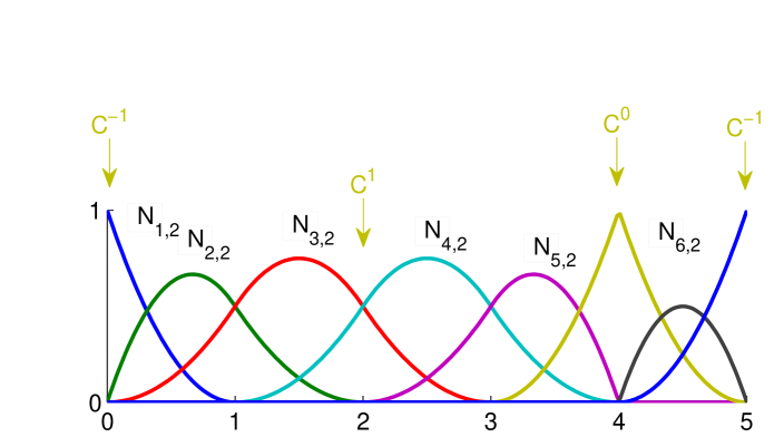
Figure 1: Quadratic ($p=2$) B-spline basis functions for an open non-uniform knot vector $\Xi=\{0,0,0,1,2,3,4,4,5,5,5\}$. Note the flexibility in the construction of basis functions with varying degrees of regularity.

NURBS basis functions are defined as

$$R_{i,p}(\xi)=\frac{N_{i,p}(\xi)w_{i}}{W(\xi)}=\frac{N_{i,p}(\xi)w_{i}}{\sum_{j=1}^{n}N_{j,p}(\xi)w_{j}},$$ (3)

where $N_{i,p}(\xi)$ denotes the $i$th B-spline basis function of order $p$ and $w_{i}$ are a set of $n$ positive weights. Selecting appropriate values for the $w_{i}$ permits the description of many different types of curves including polynomials and circular arcs. For the special case in which $w_{i}=c,i=1,2,\ldots,n$ the NURBS basis reduces to the B-spline basis. Note that for simple geometries, the weights can be defined analytically see e.g., [56]. For complex geometries, they are obtained from CAD packages such as Rhino [57].

Given two knot vectors (one for each direction) $\Xi=\{\xi_{1},\xi_{2},\ldots,\xi_{n+p+1}\}$ and $\mathscr{H}=\{\eta_{1},\eta_{2},\ldots,\eta_{m+q+1}\}$ and a control net $\mathbf{B}_{i,j}\in\mathds{R}^{d}$, a tensor-product NURBS surface is defined as

$$\mathbf{S}(\xi,\eta)=\sum_{i=1}^{n}\sum_{j=1}^{m}R_{i,j}^{p,q}(\xi,\eta)\mathbf{B}_{i,j}$$ (4)

where $R_{i,j}^{p,q}$ are given by

$$R_{i,j}^{p,q}(\xi,\eta)=\frac{N_{i}(\xi)M_{j}(\eta)w_{i,j}}{\sum_{\hat{i}=1}^{n}\sum_{\hat{j}=1}^{m}N_{\hat{i}}(\xi)M_{\hat{j}}(\eta)w_{\hat{i},\hat{j}}}$$ (5)

In the same manner, NURBS solids are defined as

$$\mathbf{S}(\xi,\eta,\zeta)=\sum_{i=1}^{n}\sum_{j=1}^{m}\sum_{k=1}^{l}R_{i,j,k}^{p,q,r}(\xi,\eta,\zeta)\mathbf{B}_{i,k,j}$$ (6)

where $R_{i,j,k}^{p,q,r}$ are given by

$$R_{i,j,k}^{p,q,r}(\xi,\eta,\zeta)=\frac{N_{i}(\xi)M_{j}(\eta)P_{k}(\zeta)w_{i,j,k}}{\sum_{\hat{i}=1}^{n}\sum_{\hat{j}=1}^{m}\sum_{\hat{k}=1}^{l}N_{\hat{i}}(\xi)M_{\hat{j}}(\eta)P_{\hat{k}}(\zeta)w_{\hat{i},\hat{j},\hat{k}}}$$ (7)

Derivatives of the B-splines and NURBS basis functions can be find elsewhere e.g., [1, 2].

3 Automatic generation of cohesive elements

3.1 Knot insertion

It should be emphasized that knot insertion does not change the B-spline curves or surfaces geometrically but a direct influence on the continuity of the approximation where knots are repeated. Let us consider a knot vector defined by $\Xi=\{\xi_{1},\xi_{2},\ldots,\xi_{n+p+1}\}$ with the corresponding control net denoted by $\mathbf{B}$. A new extended knot vector given by $\bar{\Xi}=\{\bar{\xi}_{1}=\xi_{1},\bar{\xi}_{2},\ldots,\bar{\xi}_{n+m+p+1}=\xi_{n+p+1}\}$ is formed where $m$ knots are added. The $n+m$ new control points $\bar{\mathbf{B}}_{i}$ are formed from the original control points by

$$\bar{\mathbf{B}}_{i}=\alpha_{i}\mathbf{B}_{i}+(1-\alpha_{i})\mathbf{B}_{i-1}$$ (8)

where

$$\alpha_{i}=\begin{cases}1&1\leq i\leq k-p,\\ \displaystyle\frac{\bar{\xi}-\xi_{i}}{\xi_{i+p}-\xi_{i}}&k-p+1\leq i\leq k\\ 0&k+1\leq i\leq n+p+2\end{cases}$$ (9)

Considering a quadratic B-spline curve with knot vector $\Xi=\{0,0,0,0.5,1,1,1\}$ and control points as shown in Fig. 2 (left). On the right of the same figure, two new knots $\xi=0.25$ and $\xi=0.75$ were added. Consequently, two new control points were formed. Although the curve is not changed geometrically and parametrically, the basis functions are now richer and may be more suitable for the purpose of analysis.

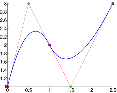
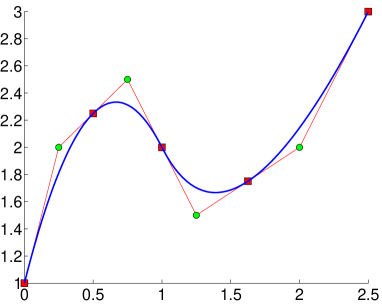
Figure 2: Knot insertion on a quadratic B-spline curve. The curve is not changed geometrically. Control points are denoted by filled green circles. Points corresponding to the knot values are denoted by red circles. These points divide the curve into segments or elements from an analysis standpoint.

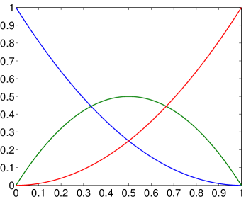
(a) $\Xi=\{0,0,0,1,1,1\}$

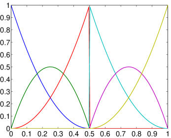
(b) $\Xi^{\prime}=\{0,0,0,0.5,0.5,0.5,1,1,1\}$

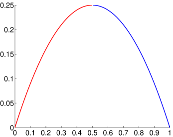
(c) B-spline curve after knot insertion

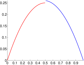
(d) B-spline curve with $\mathbf{B}^{\prime}_{4}$ moved slightly the original position

Figure 3: $p+1$ times knot insertion for a quadratic B-spline curve to introduce a $C^{-1}$ discontinuity at $\xi=0.5$.

Let us now consider a quadratic B-spline defined using $\Xi=[0,0,0,1,1,1]$. The three basis functions for this curve are given in Fig. (3a). Now suppose that we need to have a discontinuity at $\xi=0.5$. This can be achieved by inserting a new knot $\bar{\xi}=0.5$ three ($=p+1$) times. The new knot vector is then given by $\Xi^{\prime}=[0,0,0,0.5,0.5,0.5,1,1,1]$ and the new basis functions are shown in Fig. (3b). Let us build a B-spline curve with the control net defined by $\mathbf{B}$ as shown in Eq. (10). The new control net that is defined by $\mathbf{B}^{\prime}$ is also given in Eq. (10).

$$\mathbf{B}=\begin{bmatrix}0.0&0.0\\ 0.5&0.5\\ 1.0&0.0\end{bmatrix},\quad\mathbf{B}^{\prime}=\begin{bmatrix}0.00&0.00\\ 0.25&0.25\\ 0.50&0.25\\ 0.50&0.25\\ 0.75&0.25\\ 1.00&0.00\\ \end{bmatrix}.$$ (10)

where it should be noted that $\mathbf{B}^{\prime}_{3}=\mathbf{B}^{\prime}_{4}$. The B-spline curve corresponds to the original and new basis is the same and given in Fig. (3c). Imagine now that point $\mathbf{B}^{\prime}_{4}$ slightly moves vertically, the resulting B-spline curve with a strong discontinuity at $x=0.5$ is plotted in Fig. (3d). This technique of inserting knot values $p+1$ times was used in [39] to model the decohesion of material interfaces. The application of this method in two/three dimensions resemble the usage of zero-thickness interface elements by doubling nodes in the FE framework.

We demonstrate the technique to generate a discontinuity into a NURBS surface by a simple example. The studied surface is a square of $10\times 10$ and suppose that one needs a horizontal discontinuity line in the middle of the square as shown in Fig. (4a). The coarsest mesh consists of one single bi-linear NURBS element with $\Xi=\mathscr{H}=\{0,0,1,1\}$ and $p=q=1$. To insert the desired discontinuity, the following steps are performed: (1) perform order elevation to $p=q=2$; (2) perform knot insertion for $\mathscr{H}$, the new knot is $\mathscr{H}=\{0,0,0,0.5,0.5,0.5,1,1,1\}$ (Fig. (4b)); and (3) perform knot insertion to refine the mesh if needed. In Fig. (4c,d) the duplicated control points were moved upward to show the effect of discontinuity. In order to use these duplicated nodes in a FE context, one can put springs connecting each pair of nodes or employ zero-thickness interface elements. In this manuscript the latter is used. With a small amount of effort, the connectivity matrix for the interface elements can be constructed using a simple Matlab code as given in Listing LABEL:list-1D. It is obvious that, due to the simplification made in line 2 of Listing LABEL:list-1D, this code snippet applies only for a horizontal/vertical discontinuity line. However, it is straightforward to extend this template code to general cases by changing line 2. Such refinements are certainly problem dependent and hence not provided here. We refer to Fig. (5) for one example of a curved composite panel made of two plies.

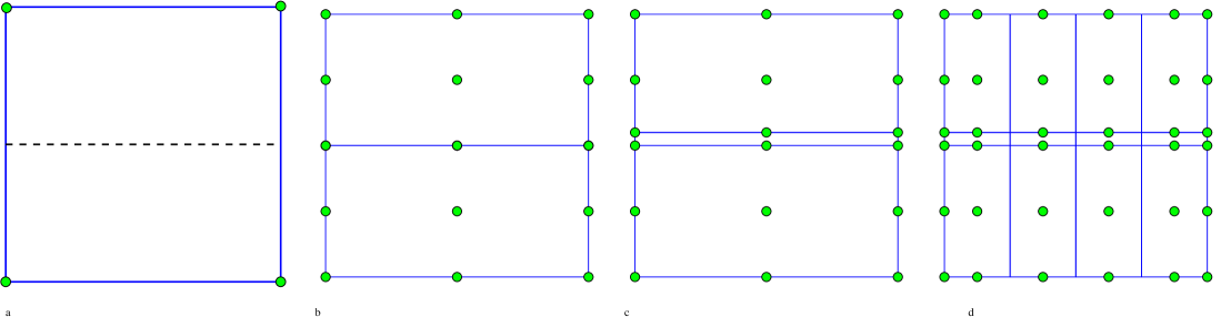
Figure 4: Example of introducing a horizontal discontinuity in a NURBS surface.

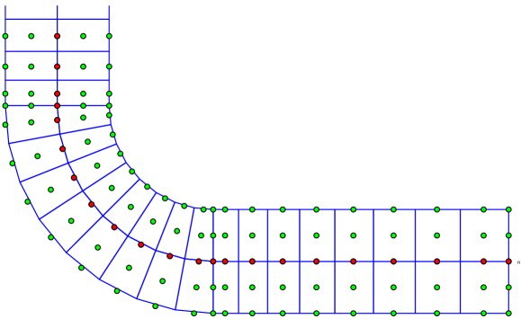
Figure 5: L-shaped composite sample of two plies with a fillet modeled with a bi-quadratic NURBS: red circles denote duplicated nodes. For this case, it suffices to find the index of node S–the first node on the discontinuity curve. By virtue of the tensor-product nature of NURBS, the indices of other discontinuity nodes can then be found with ease.

⬇

[ielements] = buildIGA1DMesh (uKnot,p);

delaminationNodes = find(abs(controlPts(:,2) - 5 ) <1e-10);

mm = 0.5*length(delaminationNodes);

lowerNodes = delaminationNodes(1:mm);

upperNodes = delaminationNodes(mm+1:end);

iElements = zeros(noElemsU,2*(p+1));

for i=1:noElemsU

sctr = ielements(i,:);

iElements(i,1:p+1) = lowerNodes(sctr);

iElements(i,p+2:end) = upperNodes(sctr);

end

⬇

delaminationNodes = find(abs(controlPts(:,3) -b/2 ) <1e-10);

mm = 0.5*length(delaminationNodes);

lowerNodes = delaminationNodes(1:mm);

upperNodes = delaminationNodes(mm+1:end);

% noElemsU=number of elements along X-dir

iElements = zeros(noElemsU*noElemsV,2*(p+1)*(q+1));

iElementS = generateIGA2DMesh (uKnot,vKnot,noPtsX,noPtsY,p,q);

for e=1:noElemsU*noElemsV

iElements(e,1:(p+1)*(q+1)) = lowerNodes(iElementS(e,:));

iElements(e,(p+1)*(q+1)+1:end) = upperNodes(iElementS(e,:));

end

The technique introduced so far can be straightforwardly extended to three dimensions, see Listing LABEL:list-2d and Fig. (6) for an example. The discontinuity surface lies in the $X-Y$ plane. Line 7 of this Listing builds the element connectivity array for a 2D NURBS mesh, we refer to [34] for a detailed description of these Matlab functions. These pre-processing techniques are implemented in our open source Matlab IGA code named MIGFEM, desribed in [34], which is available at https://sourceforge.net/projects/cmcodes/. In order to support IGA codes which are based on the Bézier extraction [58, 59], see also Section 4.5, MIGFEM computes the 1D, 2D and 3D Bézier extractors. In summary the pre-processing code writes to a file with (1) coordinates of control points (including duplicated ones), (2) connectivity of continuum elements, (3) connectivity of interface elements, (4) 2D/3D Bézier extractors for continuum elements and (5) 1D/2D extractors for interface elements. It should be emphasized that inserting interface elements into a Lagrange FE mesh is a time-consuming task even with commercial FE packages. Due to that fact, a free mesh generator for cohesive modeling was developed by the first author and presented in [60].

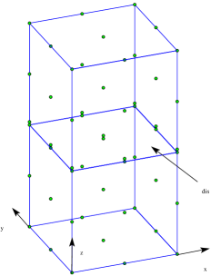
Figure 6: A 3D bar with a discontinuity surface in the middle: modeled by a tri-quadratic NURBS solid.

Remark 3.1.

In the proposed framework, interface elements are inserted a priori, therefore delaminations only grow along predefined paths. For laminates built up by plies of unidirectional fiber reinforced composites, the fracture toughness of the plies is much greater than the fracture toughness of the ply interfaces. Therefore, delaminations only grow along the ply interfaces which are known a priori. And that justifies our assumption.

4 Finite element formulation

4.1 Isogeometric analysis

According to the IGA the field variable (which is, in this paper, the displacement field) is approximated by the same B-spline/NURBS basis functions used to exactly represent the geometry. Therefore, in an IGA context, one writes for the geometry and displacement field, respectively

$$\mathbf{x} =N_{I}(\boldsymbol{\xi})\mathbf{x}_{I}$$ (11a)

$$u_{i} =N_{I}(\boldsymbol{\xi})u_{iI}$$ (11b)

where $\mathbf{x}_{I}$ are the nodal coordinates, $u_{iI}$ is the $i$ ($i=1,2,3$) component of the displacement at node/control point $I$ and $N_{I}$ denotes the shape functions which are the B-spline/NURBS basis functions described in Section 2.

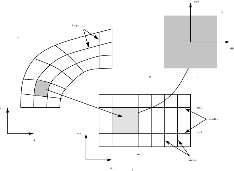
Figure 7: Definition of domains used for integration in isogeometric analysis. Elements are defined in the parametric space as non-zero knot spans, $[\xi_{i},\xi_{i+1}]\times[\eta_{j},\eta_{j+1}]$ and elements in the physical space are images of their parametric counterparts.

Elements are defined as non-zero knot spans, see Fig. (7), which are elements in the parameter space (denoted by $\hat{\Omega}_{e}$). Their images in the physical space obtained via the mapping, see Eq. (11), are called elements in the physical space (denoted by $\Omega_{e}$) that resemble the familiar Lagrange elements. From our experiences, it is beneficial to work with elements in the parameter space. Numerical integration is also performed on a parent domain as in Lagrange FEs.

4.2 FE discrete equations

The semi-discrete equation for a solid with cohesive cracks is given by

$$\mathbf{M}\mathbf{a}=\mathbf{f}^{\textrm{ext}}-\mathbf{f}^{\textrm{int}}-\mathbf{f}^{\textrm{coh}}$$ (12)

where $\mathbf{a}$ is the acceleration vector, $\mathbf{M}$ denotes the consistent mass matrix, $\mathbf{f}^{\textrm{ext}}$ is the external force vector , the internal force vector is denoted as $\mathbf{f}^{\textrm{int}}$ and the cohesive force vector $\mathbf{f}^{\textrm{coh}}$. The elemental mass matrix, external and internal force vectors are computed from contributions of continuum elements and given by

$$\mathbf{M}_{e} =\int_{\Omega_{e}}\rho\mathbf{N}^{\mathrm{T}}\mathbf{N}\mathrm{d}\Omega_{e}$$ (13)

$$\mathbf{f}^{\textrm{int}}_{e} =\int_{\Omega_{e}}\mathbf{B}^{\mathrm{T}}\boldsymbol{\sigma}\mathrm{d}\Omega_{e}$$ (14)

$$\mathbf{f}^{\textrm{ext}}_{e} =\int_{\Omega_{e}}\rho\mathbf{N}^{\mathrm{T}}\mathbf{b}\mathrm{d}\Omega_{e}+\int_{\Gamma_{t}^{e}}\mathbf{N}^{\mathrm{T}}\bar{\mathbf{t}}\mathrm{d}\Gamma_{t}^{e}$$ (15)

where $\rho$ is the density, $\Omega_{e}$ is the element domain, $\Gamma_{t}^{e}$ is the element boundary that overlaps with the Neumann boundary, $\mathbf{b}$ and $\bar{\mathbf{t}}$ are the body forces and traction vector, respectively. The shape function matrix and the strain-displacement matrix are denoted by $\mathbf{N}$ and $\mathbf{B}$; $\boldsymbol{\sigma}$ is the Cauchy stress vector.

The cohesive force vector is computed by assembling the contribution of all interface elements. It is given by for an interface element $ie$

$$\begin{split}\mathbf{f}^{\textrm{coh}}_{ie,+}&=\int_{\Gamma}\mathbf{N}^{\mathrm{T}}_{\text{int}}\mathbf{t}^{\mathrm{c}}\mathrm{d}\Gamma\\ \mathbf{f}^{\textrm{coh}}_{ie,-}&=-\int_{\Gamma}\mathbf{N}^{\mathrm{T}}_{\text{int}}\mathbf{t}^{\mathrm{c}}\mathrm{d}\Gamma\end{split}$$ (16)

in which $\mathbf{t}^{c}$ denotes the cohesive traction, $\mathbf{N}_{\text{int}}$ represents the shape function matrix of interface elements. The subscripts +/- denote the upper and lower faces of the interface element.

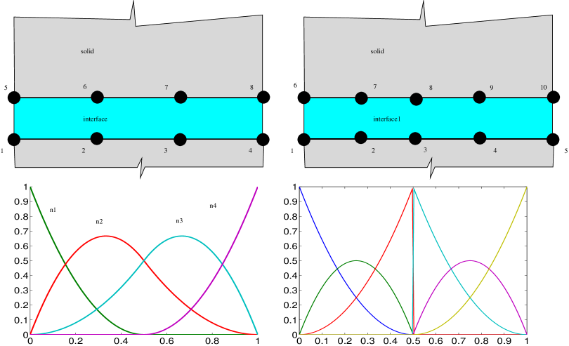
Figure 8: Illustration of $C^{p-1}$ NURBS interface elements (left) and $C^{0}$ NURBS interface elements (right): For $C^{p-1}$ elements, the connectivity of the first element is $[1,2,3,5,6,7]$ while the connectivity of the second element is $[2,3,4,6,7,8]$.

The displacement of the upper and lower faces of an interface element, let say the first element in Fig. (8)-left read

$$\begin{split}\mathbf{u}^{+}&=N_{1}(\xi)\mathbf{u}_{5}+N_{2}(\xi)\mathbf{u}_{6}+N_{3}(\xi)\mathbf{u}_{7}\\ \mathbf{u}^{-}&=N_{1}(\xi)\mathbf{u}_{1}+N_{2}(\xi)\mathbf{u}_{2}+N_{3}(\xi)\mathbf{u}_{3}\\ \end{split}$$ (17)

with $N_{I}$ ($I=1,2,3,4$) are the quadratic NURBS shape functions. Figure 8 also explains the difference between $C^{p-1}$ and $C^{0}$ high order elements–for the same number of elements, $C^{p-1}$ meshes have less nodes. We refer to [1] for more information on this issue. The latter was used in [53] with B-spline basis for 2D delamination analysis.

Having defined the displacement of the upper and lower faces of the interface, it is able to compute the displacement jump as

$$\llbracket\mathbf{u}(\mathbf{x})\rrbracket\equiv\mathbf{u}^{+}-\mathbf{u}^{-}=\mathbf{N}_{\text{int}}(\mathbf{u}^{+}-\mathbf{u}^{-})$$ (18)

where

$$\mathbf{N}_{\text{int}}=\begin{bmatrix}N_{1}&0&N_{2}&0&N_{3}&0\\ 0&N_{1}&0&N_{2}&0&N_{3}\end{bmatrix},\quad\mathbf{u}^{+}=\begin{bmatrix}u_{x5}&u_{y5}&u_{x6}&u_{y6}&u_{x7}&u_{y7}\end{bmatrix}^{\mathrm{T}}$$ (19)

The displacement jump will be inserted into a cohesive law (or traction-separation law) to compute the corresponding traction $\mathbf{t}^{c}$. We refer to [40, 41, 42] and references therein for other aspects of interface cohesive elements. The implementation for three dimensional problems i.e., 2D interface elements is straightforward, for example in Eq. (17), instead of using univariate NURBS basis one uses bivariate basis $N_{I}(\xi,\eta)$.

4.3 Cohesive laws

In this work, we adopt the damage-based bilinear cohesive law developed in [61, 62]. This is a cohesive law in which the fracture toughness is a phenomenological function, rather than a material constant, of mode mixity as formulated by Benzeggagh and Kenane [63]. Herein we briefly recall the cohesive law of which implementation details can be found in [64]. Denoting $d$ as the damage variable ($0\leq d\leq 1$), the cohesive law reads in the local coordinate system attached to the interface elements

$$\mathbf{t}^{c}_{l}=(1-d)K\llbracket\mathbf{u}\rrbracket_{l}$$ (20)

where $K$ is the dummy stiffness. The damage variable $d$ is a function of the equivalent displacement jump, the onset $[\![{u}]\!]_{\text{eq}}^{0}$ and the propagation equivalent displacement jump $[\![{u}]\!]_{\text{eq}}^{f}$. The onset $[\![{u}]\!]_{\text{eq}}^{0}$ is a function of $K$, the mode mixity and the normal and shear strength $\tau^{0}_{1}$ and $\tau^{0}_{3}$. The propagation displacement jump $[\![{u}]\!]_{\text{eq}}^{f}$ is a function of $[\![{u}]\!]_{\text{eq}}^{0}$, mode I and II fracture toughness $G_{Ic}$, $G_{IIc}$, the mode mixity and $\eta$ which is a curve fitting value for fracture toughness tests performed by Benzeggagh and Kenane [63].

4.4 Numerical integration

In this manuscript, full Gaussian integration schemes are used. Precisely, for 2D solid elements of order $p\times q$, a $(p+1)\times(q+1)$ Gauss quadrature rule is adopted and for cohesive elements of order $p$, a $(p+1)$ Gauss scheme is utilized. A similar rule was used for 3D solid elements and 2D cohesive elements.

4.5 Implementation aspects

There are at least two approaches to incorporating IGA into existing FE codes–with and without using the Bézier extraction. The former, which relies on the Bézier decomposition technique, was developed in [58, 59] and provides data structures (the so-called Bézier extractor sparse matrices) that facilitate the implementation of IGA in existing FE codes. Precisely, the shape functions of IGA elements are the Bernstein polynomials (defined on the standard parent element) multiplied by the extractors. We refer to [34] for a discussion on both techniques.

For curved geometries, the post-processing of IGA is more involved than Lagrange FEs due to two reasons (1) some control points locate outside the physical domain (hence the computed displacements at control points are not nodal values) and (2) existing post-processing techniques cannot be applied directly to NURBS meshes. Interested reader can refer to [34] for a discussion on some post-processing techniques for IGA. For completeness we discuss briefly one technique here for 2D problems. First, a visualization mesh which consists of four-noded quadrilateral elements is constructed. The nodes of this mesh are the intersections of the $\xi$ and $\eta$ knot lines in the physical space. We then extrapolate the quantities at Gauss points to these nodes and perform nodal averaging if necessary. Figure 9 summarizes the idea.

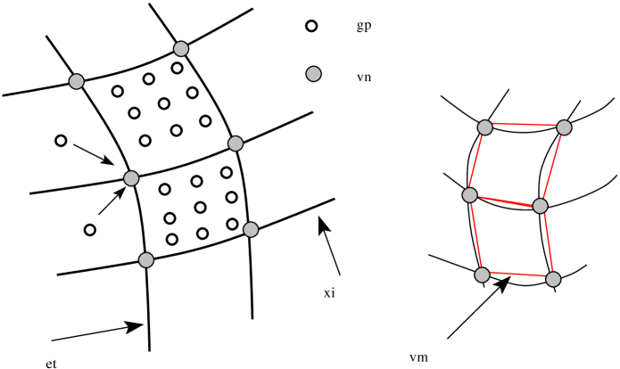
Figure 9: Post-processing in Isogeometric Analysis.

5 Examples

Since we are introducing a computational framework for delamination analyses rather than a detailed study of the delamination behaviour of composite materials, intralaminar damage (matrix cracking and fiber damage) is not taken into account leading to an orthotropic elastic behaviour assumption for the plies. Note that matrix cracking can however be efficiently modeled using extended finite elements as shown in [65, 64] and can be incorporated in our framework without major difficulties. Besides, inertia effects are also skipped. In order to trace equilibrium curves we use either a displacement control (for problems without snapbacks) and the energy-based arc-length control [66, 67]. Interested reader can refer to [53, 65] for the computer implementation aspects of this arc-length solver. A full Newton-Raphson method was used to solve the discrete equilibrium equations. Unless otherwise stated, a geometrically linear formulation is adopted. We use a C++ code [68] for computations since Matlab is not suitable for this purpose. Whenever possible, validation against theoretical solutions are provided.

Four numerical examples are provided including

• Mixed mode bending test (MMB), 2D simple geometry, implementation verification test;

• L-shaped specimen, single and multiple delamination, NURBS curved geometry;

• 3D double cantilever beam, to verify the implementation;

• Singly curved thick-walled laminate, 3D curved geometry.

And in an extra example, we present NURBS parametrization for other commonly used composite structures–glare panel with a circular initial delamination, open hole laminate and doubly curved composite panel.

5.1 Mixed mode bending test (MMB)

Figure 10 shows the mixed mode bending test of which the geometry data are $L=100$ mm, $h=3$ mm; the beam thickness $B$ is equal to 10 mm; the initial crack length is $a_{0}=20$ mm. The plies are modeled with isotropic material to make a fair comparison with analytical solutions [69] which are valid for isotropic materials only. The properties for the isotropic material are $E=150$ GPa and $\nu=0.25$. The properties for the cohesive elements are $G_{Ic}=0.352$ N/mm, $G_{IIc}=1.45$ N/mm and $\tau^{0}_{1}=80$ MPa, $\tau^{0}_{3}=60$ MPa. The interface stiffness is $K=10^{6}$ N/mm³ and $\eta=1.56$. In order to prevent interpenetration of the two arms, in addition to cohesive elements, frictionless contact elements are placed along the initial crack. The loads applied are $P_{1}=2Pc/L$ and $P_{2}=P(2c+L)/L$, where $L$ is the beam length, $c$ is the lever arm length, and $P$ is the applied load. From these relationships, it is clear that the applied loads $P_{1}$ and $P_{2}$ are proportional i.e., $P_{2}/P_{1}=(2c+L)/L$. We choose $c=43.72$ mm so that the mixed-mode ratio $G_{I}/G_{II}$ is unity. The external force vector is therefore $\mathbf{f}^{\text{ext}}=\lambda[1,-2.1436]^{\mathrm{T}}$ (a unit force was assigned to $P_{1}$) in which the variable load scale $\lambda$ is solved together with the nodal displacements using the energy based arc-length method [66, 67, 53].

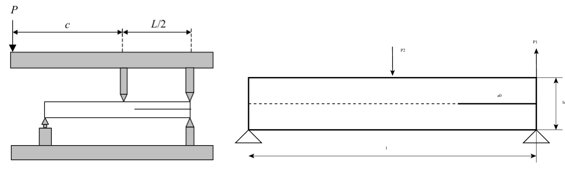
Figure 10: Mixed Mode Bending (MMB): geometry and loading.

5.1.1 Geometry and mesh

For those who are not familiar to B-splines/NURBS, we present how to build the beam geometry using B-splines. It is obvious that the beam can be exactly represented by a bilinear B-spline surface with 4 control points locating at its four corners. The Matlab code for doing this is lines 1–9 in Listing LABEL:list-mmb. Next, the B-spline is order elevated to the order that suits the analysis purpose, see line 10 of the same Listing. The delamination path locates in the midline of the beam i.e., $\eta=0.5$ and note that $q=2$, in order to introduce a discontinuity one simply has to insert $0.5$ three ($=q+1$) times into knot vector $\mathscr{H}$ (knot vector which is perpendicular to the delamination plane). For point load $P_{2}$ one needs a control point at the location of the force which corresponding to insert 0.5 three times (equals $p=3$) into knots $\Xi$. Line 13 does exactly that. In order to differentiate cohesive elements and contact elements (remind that contact elements are put along the initial crack to prevent interpenetration), a knot $1-a_{0}/L$ is added to $\Xi$ $p$ times (see line 14). The final step is to perform a $h$-refinement to refine the mesh and extract element connectivity data for the interface elements using the code given in Listing LABEL:list-1D.

⬇

controlPts = zeros(4,2,2);

controlPts(1:2,1,1) = [0;0]; % L=length of beam

controlPts(1:2,2,1) = [L;0]; % W=height of beam

controlPts(1:2,1,2) = [0;W];

controlPts(1:2,2,2) = [L;W];

controlPts(4,:,:) = 1; % weights = 1: B-splines

uKnot = [0 0 1 1];

vKnot = [0 0 1 1];

solid = nrbmak(controlPts,{uKnot vKnot}); % build the initial NURBS object

solid = nrbdegelev(solid,[2 1]); % evaluate order to cubic-quadratic surface

% h-refinement in Y direction to make sure it is C^{-1} along the

% delamination path. The multiplicity must be q+1. Also insert knot to have a C^0

% at loading point

solid = nrbkntins(solid,{[0.5 0.5 0.5] [0.5 0.5 0.5]});

solid = nrbkntins(solid,{[1-a0/L 1-a0/L 1-a0/L] []});% insert for intitial crack

5.1.2 Analyses with varying basis orders

We use meshes with two elements along the thickness direction and the basis order along this direction is fixed to 2 (quadratic basis). The notation $2\times 128$ B$2\times 3$ indicates a mesh of $2\times 128$ elements of orders $2\times 3$. The order of basis functions along the length direction, $p$, varies from two to five. Firstly we perform a mesh convergence test for quartic-quadratic elements and the result is given in Fig. (11a). Mesh $2\times 64$ is simply too coarse to accurately capture the cohesive zone and mesh $2\times 128$ is sufficient to get a reasonable result. Next, the mesh density is fixed at $2\times 128$ and $p$ is varied from 2 to 5, the result is plotted in Fig. (11b). We refer to [53] for a throughout study on the excellent performance of high order B-splines elements compared to low order Lagrange finite elements for delamination analyses.

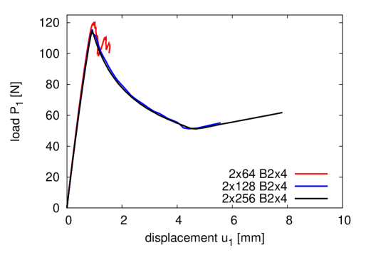
(a)

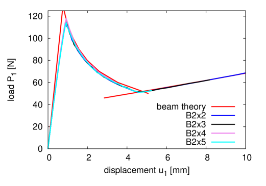
(b)

Figure 11: Mixed Mode Bending (MMB): (a) mesh convergence test and (b) varying basis order in the length direction on meshes of $2\times 128$ elements.

5.2 L-shaped composite panel with a fillet

For the second example, we analyze the L-shaped composite specimen which was studied in [55, 54] using Lagrange finite elements. The geometry and loading configuration is given in Fig. (12). Contrary to the previous example, in this example NURBS surfaces are used to exactly represent the curved geometry (to be precise circular arcs). The structure is built up by 15 plies of a unidirectional fiber reinforced carbon/epoxy material. The plies are oriented in alternating 0^∘ and 90^∘ orientation, where the angle is measured from the $xy$ plane. The inner ply and the outer ply are oriented in the 0^∘ direction. Material constants are given in Table 1 which are taken from [55, 54]. A plane strain condition is assumed. For this problem, unless otherwise stated, we use bi-quadratic NURBS elements for the continuum and quadratic NURBS interface elements for the delamination.

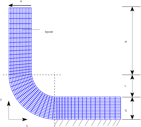
Figure 12: L-shaped specimen: boundary and geometry data. There are 15 plies (0^∘ and 90^∘). The ply orientation is measured with respect to the $x-y$ plane.

$E_{11}$	$E_{22}=E_{33}$	$G_{12}=G_{13}$	$\nu_{12}=\nu_{13}$	$\nu_{23}$
139.3 GPa	9.72 GPa	5.59 GPa	0.29	0.40
$G_{Ic}$	$G_{IIc}$	$\tau^{0}_{1}$	$\tau^{0}_{3}$	$\mu$
0.193 N/mm	0.455 N/mm	60.0 MPa	80.0 MPa	2.0

Table 1: L-shaped specimen: material properties.

5.2.1 Geometry and mesh

The L-shaped geometry can be exactly represented by a quadratic-linear NURBS surface as shown in Fig. (13) that consists of $7\times 2$ control points. The Matlab code used to build the NURBS is given in Listing LABEL:list:lshape-geo. It is easy to vary the number of plies (see line 4 of the same Listing). Listing LABEL:list:lshape-insert gives code to perform $p$-refinement (to a bi-quadratic NURBS surface) and knot insertion at ply interfaces (two times) to create $C^{0}$ lines so that the strain field is discontinuous across the ply interfaces. Next, knot insertion is performed again to generate discontinuity lines at the desired ply interfaces. Two cases are illustrated in the code–interface elements locate along the interface between ply 5 and 6 (line 10) and interface elements at every ply interfaces (line 12-16).

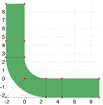
Figure 13: L-shaped specimen: quadratic-linear NURBS geometry with control points (filled circles) and control polygon.

⬇

H = 6.4;

R = 2.55;

R0 = 2.25;

no = 15; % number of plies

t = R0/no;% ply thickness

% initial mesh- quadratic x linear

uKnot = [0 0 0 1 1 2 2 3 3 3]; uKnot = uKnot/max(uKnot);

vKnot = [0 0 1 1];

controlPts = zeros(4,7,2);

controlPts(1:2,1,1) = [H+R;0]; controlPts(1:2,1,2) = [H+R;-R0];

controlPts(1:2,2,1) = [(H+R)/2;0]; controlPts(1:2,2,2) = [(H+R)/2;-R0];

controlPts(1:2,3,1) = [R;0]; controlPts(1:2,3,2) = [R;-R0];

controlPts(1:2,4,1) = [0;0]; controlPts(1:2,4,2) = [-R0;-R0];

controlPts(1:2,5,1) = [0;R]; controlPts(1:2,5,2) = [-R0;R];

controlPts(1:2,6,1) = [0;(H+R)/2]; controlPts(1:2,6,2) = [-R0;(H+R)/2];

controlPts(1:2,7,1) = [0;H+R]; controlPts(1:2,7,2) = [-R0;H+R];

fac = 1/sqrt(2);

controlPts(4,:) = 1; % all weights are units except two points

controlPts(4,4,1) = controlPts(4,4,2) = fac;

controlPts(1:2,4,1) = fac*controlPts(1:2,4,1);

controlPts(1:2,4,2) = fac*controlPts(1:2,4,2);

solid = nrbmak(controlPts,{uKnot,vKnot}); %% build NURBS object

⬇

solid = nrbdegelev(solid,[0 1]); % evaluate order to bi-quadratic

% knot insertion to have C^0 lines at ply interfaces

knots=[];

for ip=1:no-1

dd = t*ip/R0;

knots = [knots dd dd]; % multiplicity = order + 1

end

solid = nrbkntins(solid,{[] knots});

% knot insertion to have C^{-1} line at interface between plies 5 and 6

solid = nrbkntins(solid,{[] 5*t/R0});

% if interface elements are placed at all ply interfaces, then

knots=[];

for ip=1:no-1

dd = t*ip/R0;

knots = [knots dd];

end

solid = nrbkntins(solid,{[] knots});

% h-refinement along \xi direction to have a refined model for FEA

5.2.2 Single delamination with and without initial cracks

Delamination of the interface between ply five and six is first analyzed. Note that at other ply interfaces, there is no cohesive elements. Firstly, the case of no initial cracks is considered. One layer of elements is used for each ply. The contour plot of damage on the deformed shape is given in Fig. (14) and the response in terms of reaction-displacement curve is plotted in Fig. (15). There is a sharp snap-back that corresponds to an unstable delamination growth. After the delamination reaches a certain size, stable delamination growth is observed as shown by the increasing part of the load-displacement curve. This is in good agreement with the semi-analytical analysis in [55]. The excellent performance of the energy-based arc-length control for responses with sharp snap-backs has been demonstrated elsewhere e.g., [53, 65], we therefore do not give an discussion on this issue.

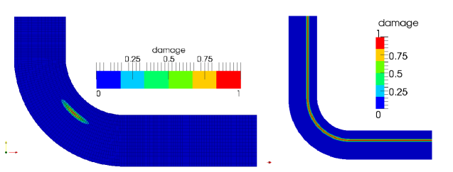
Figure 14: L-shaped specimen: delamination configurations at the peak (left) and when the delamination reached the two ends (right).

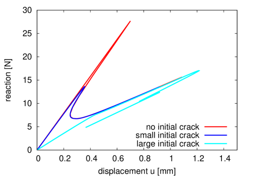
Figure 15: L-shaped specimen with one single delamination between ply 5 and 6: without initial cracks, with an small and large initial crack.

Let assume now that there is an initial crack lying on the interface between ply 5 and 6, see Fig. (16). The initial crack is a part of the NURBS curve that defines the interface of ply 5 and 6. In this case the geometry modeling procedure is more involved and follows the steps given in Listing LABEL:list:lshape-init-crack. The extra step is to perform a point inversion algorithm [56] to find out the parameters $\xi_{1}$ and $\xi_{2}$ that correspond to points $\mathbf{x}_{1}$ and $\mathbf{x}_{2}$–the tips of the initial crack. After that $\xi_{1},\xi_{2}$ are inserted twice (remind that the NURBS basis order along the $\xi$ direction is two).

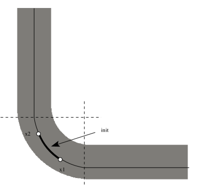
Figure 16: L-shaped specimen with one initial crack.

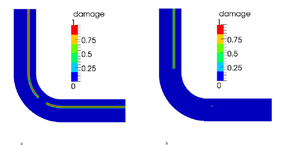
Figure 17: L-shaped specimen with one initial crack: delamination configurations for the case of small initial crack (a) and large initial crack (b).

⬇

% code from Listing 4 to build the NURBS surface

% code from Listing 5 to create C^0 and C^{-1} lines

% point inversion to find parametric values xi1 and xi2 that correspond to

% points x_1 and x_2 defining the initial crack.

% insert xi1 and xi2 2 times (p=) to have C^0 at x_1 and x_2

solid = nrbkntins(solid,{[xi1 xi1 xi2 xi2] []});

% h-refinement along \xi direction to have a refined model for FEA

Remark 5.2.

Point inversion for NURBS curves concerns the computation of parameter $\bar{\xi}$ that corresponds to a point $\bar{\mathbf{x}}$ such that $N_{I}(\bar{\xi})\mathbf{x}_{I}=\bar{\mathbf{x}}$ where $\mathbf{x}_{I}$ denote the control points of the curve. Generally, a Newton-Raphson iterative method is used, we refer to [56] for details.

Two cases, one with a small initial crack and one with a large initial crack are considered. The delamination of the specimen is given in Fig. (17) and the responses are plotted in Fig. (15). For the case of a small initial crack, the response of the specimen is very similar to the case without any initial cracks, except that the peak load is smaller. For the case of a large initial crack, the delamination growth is stable. This is in good agreement with the work in [55].

5.2.3 Multiple delaminations

In order to study multiple delaminations, we place cohesive elements along all ply interfaces and one large initial crack at the interface of ply 3 and 4 (we conducted an analysis without any initial crack and found that delamination was initiated at the interface of ply 3 and 4). The analysis was performed using about 100 load increments and the computation time was 730s on a Intel Core i7 2.8GHz laptop (29 340 unknowns and 9280 elements). Figure 18 gives the response of the specimen. As can be seen, the propagation of the first delamination (from both tips of the initial crack) is stable and the growth of the second delamination (between ply 7 and 8) is unstable .

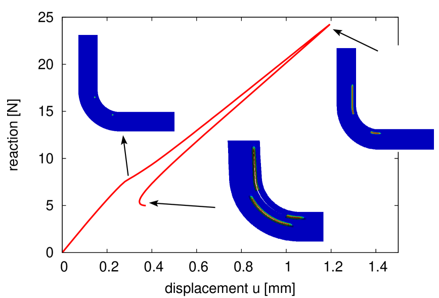
Figure 18: L-shaped specimen with one initial crack and cohesive elements at all ply interfaces: multiple delaminations.

5.3 Three dimensional double cantilever beam

As the simplest 3D delamination problem as far as geometry is concerned, we consider the 3D double cantilever beam (DCB) problem as given in Fig. (19). This example serves as a verification test for (1) verifying the implementation of 3D isogeometric interface elements and (2) validating the automatic generation of 2D isogeometric interface elements.

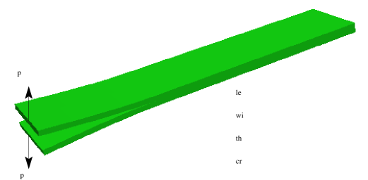
Figure 19: Three dimensional double cantilever beam: geometry and loading data.

5.3.1 Geometry and mesh

The beam geometry is represented by one single tri-linear NURBS (actually B-splines as the weights are all units), see Lines 1–5 of Listing LABEL:list:dcb-geo. Order elevation was then performed to obtain a tri-quadratic solid (line 7) followed by a knot insertion to create the discontinuity surface. Finally, $h$-refinement can be applied along any or all directions to have a refined model which is analysis suitable. Listing LABEL:list-2d is then used to build the element connectivity array for the interface elements.

⬇

uKnot = [0 0 1 1];

vKnot = [0 0 1 1];

wKnot = [0 0 1 1];

%% build NURBS object

solid = nrbmak(controlPts,{uKnot vKnot wKnot}); % controlPts = 8 corners of the beam

% evaluate order

solid = nrbdegelev(solid,[1 1 1]); % to tri-quadratic NURBS solid

% h-refinement in thickness direction to make sure it is C^{-1} along the

% delamination path. The multiplicity must be order+1.

solid = nrbkntins(solid,{[] [] [0.5 0.5 0.5]});

% insert a knot at the tip of the initial crack

solid = nrbkntins(solid,{[a0/L] [] []});

5.3.2 Analysis results

We use an isotropic material with Young modulus $E=2.1\times 10^{5}$ MPa and Poisson ratio $\nu$ = 0.3. The material constants for the cohesive law are $G_{Ic}$=0.28 N/mm, $\tau^{0}_{1}$= 27 MPa, $K=10^{7}$ N/mm³. Two layers of elements are placed along the thickness and the width direction. Figure 20 shows the deformed shape and the load-displacement curve including a comparison with the classical beam theory solution.

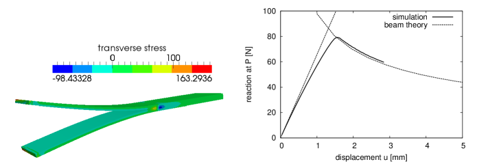
Figure 20: Three dimensional double cantilever beam: contour plot of the transverse stress on the deformed shape (magnification factor of 3).

5.3.3 Analysis results with shell elements

Next, the problem is solved using isogeometric shell elements. We refer to, for instance, [14, 15, 16] for details on isogeometric shell elements. In this section, we adopt the rotation-free Kirchhoff-Love thin shell as presented in [15]. Due to its high smoothness, NURBS are suitable for constructing $C^{1}$ shell elements without rotation degrees of freedom. In order to fix the rotation at the right end of the beam, we fix the displacements (all components) of the last two rows of control points, see Fig. (21a) and we refer to [15, 34] for details. For each ply is represented by its own NURBS surface, there is automatically a discontinuity between their interface. Therefore, generation of interface elements in this context is straightforward. Each ply is discretized by a mesh of $264\times 1$ bi-quadratic elements. The number of nodes/control points is 1596. Figure 21 gives the contour plot of damage and the load-displacement curves.

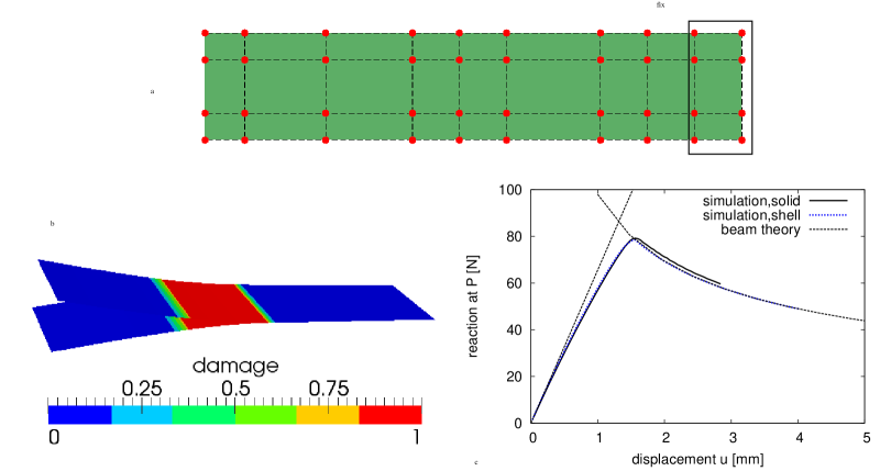
Figure 21: Three dimensional double cantilever beam modeled by shell elements: (a) B-spline mesh of one ply with fixed control points and (b) contour plot of damage on the deformed shape (magnification factor of 3) and (c) load-displacement curves.

5.4 Singly curved thick-walled laminate

As a 3D example with more complex geometry, we consider a singly curved thick-walled laminate which was studied in [70, 71]. Air-intakes of formula race cars and strongly curved regions of ship hulls provide examples for such thick-walled curved laminates designs. The geometry of the sample is given in Fig. (22). Since the geometry representation of the object of interest is the same in both CAD and FEA environment, it is very straightforward and fast to get an analysis-suitable model when changes are made to the CAD model, for instance changing the thickness $t$. This is in sharp contrary to Lagrange finite elements which uses a different geometry representation. This example also shows how a trivariate NURBS representation of a curved thick/thin-walled laminate can be built given a NURBS curve or surface. For computation, the material constants given in Table 2 are used of which the material properties of the plies are taken from [70]. The material constants for the interfaces are not provided in [70], the ones used here are therefore only for computation purposes.

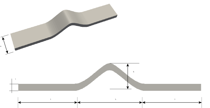
Figure 22: Singly curved thick-walled laminates: geometry configuration. The thickness $t$ is constant.

$E_{11}$	$E_{22}=E_{33}$	$G_{12}=G_{13}$	$\nu_{12}=\nu_{13}$	$\nu_{23}$
110 GPa	10 GPa	5.00 GPa	0.27	0.30
$G_{Ic}$	$G_{IIc}$	$\tau^{0}_{1}$	$\tau^{0}_{3}$	$\mu$
0.075 N/mm	0.547 N/mm	80.0 MPa	90.0 MPa	1.75

Table 2: Singly curved thick-walled laminate: material properties.

5.4.1 Geometry and mesh

The geometry of the singly curved thick-walled laminates can be built by first creating a NURBS curve as shown in Fig. (23). Next, an offset of this curve with offset distance $t$ is created using the algorithm described in [72] which ensures the offset curve has the same parametrization as its base. This allows a tensor-product surface bounded by these two curves can be constructed. Having these two curves, a B-spline surface can be constructed. Knot insertion was then made to build $C^{-1}$ lines at the ply interfaces. Finally, the cross section is extruded along the width direction. We refer to Listing LABEL:list:curved-geo for the Matlab code that produces the geometry. Again, the number of ply can be easily changed and interface elements can be placed along any ply interface. NURBS meshes of the sample are given in Fig. (24).

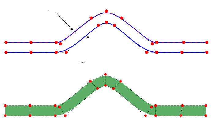
Figure 23: Singly curved thick-walled laminates: building the cross section as a B-spline surface made of the base curve and its offset. The red points denote the control points.

⬇

l = 80; L = 100; t = 10; w = 40; h = 30;

no = 4; % number of layers

uKnot = [0 0 0 1 1 2 3 4 5 6 6 7 7 7];

controlPts = zeros(4,11);

controlPts(1:2,1) = [0;0];

controlPts(1:2,2) = [0.5*l;0];

controlPts(1:2,3) = [l;0];

controlPts(1:2,4) = [l+10;0];

controlPts(1:2,5) = [l+0.5*L-8;h-3];

controlPts(1:2,6) = [l+0.5*L;h];

controlPts(1:2,7) = [l+0.5*L+8;h-3];

controlPts(1:2,8) = [l+L-10;0];

controlPts(1:2,9) = [l+L;0];

controlPts(1:2,10) = [1.5*l+L;0];

controlPts(1:2,11) = [2*l+L;0];

controlPts(4,:,:) = 1;

curve = nrbmak(controlPts,uKnot);

[oCurve,offsetPts]= offsetCurve(curve,t,alpha,beta,eps1,maxIter); % offset curve

surf = surfaceFromTwoCurves(curve, oCurve);

surf = nrbdegelev(surf,[0 1]); % evaluate order => bi-quadratic

% h-refinement in Y direction to make sure it is C^{-1} along delamination path

knots=[];

for ip=1:no-1

dd = ip/4;

knots = [knots dd dd dd];

end

surf = nrbkntins(surf,{[] knots});

solid = nrbextrude(surf, [0,0,w]); % make the solid

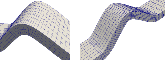
Figure 24: Singly curved thick-walled laminates: NURBS meshes.

5.4.2 2D analyses

Since the straight specimen ends were placed in the clamps of a closed-loop controlled servo-hydraulic testing machine [71], in the FE model, the straight ends are not included. The sample is subjected to a compressive force on the right end and fixed in the left end. The laminate is composed of 45 unidirectional ($0^{\circ}$) plies of carbon fiber reinforced plastic. The mesh was consisted of $40\times 45$ quartic-quadratic NURBS elements and 1760 quartic interface elements. The number of nodes is 7 020 hence the number of unknowns is 14 040. The analysis was performed in 121 load increments and the computation time was 1300s on a Intel Core i7 2.8GHz laptop. The delamination pattern and the load-displacement is given in Fig. (25). Note that no effort was made to compare the obtained result with the test given in [71] since it is beyond the scope of this paper.

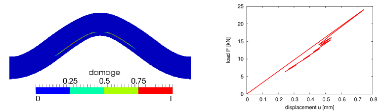
Figure 25: Singly curved thick-walled laminate under compression: delamination pattern (left) and load-displacement curve (right).

5.4.3 3D analyses

5.5 Some other models

For completeness, in this section we apply the presented isogeometric framework to other commonly encountered composite structures. In Fig. (26c), a glare panel with a circular initial delamination is given (one quarter of the panel is shown due to symmetry). The NURBS representation of the panel is given in Fig. (26a) in which the coarsest mesh that consists of $2\times 2$ quadratic-linear NURBS elements can capture the circle geometry and Fig. (26b) shows a refined mesh. Then, interface elements can be straightforwardly inserted and delamination analyses can be performed Fig. (26c,d). It should be emphasized that the chosen NURBS parametrization given in Fig. (26a) is not unique and there are singular points at the bottom left and top right corners (this, however, does not affect the analysis since no integration points are placed there).

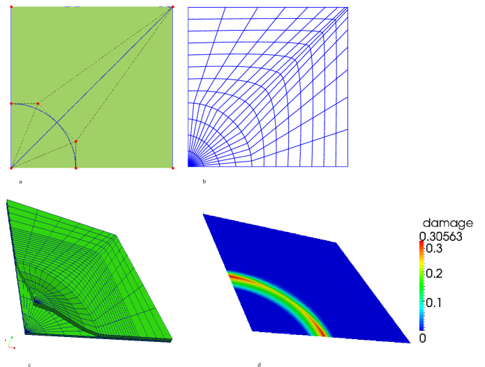
Figure 26: Glare with a circular initial delamination: (a) NURBS surface with control points and mesh (4 elements), (b) refined mesh, (c,d) deformed shape and damage plot.

Next, we present a NURBS mesh for the open hole laminate as shown in Fig. (27). The whole sample can be represented by six NURBS patches of which four patches are for the central part. In this figure, we give a parametrization that results in a so-called compatible multi-patch model. Note that across the patch interface, the basis is only $C^{0}$. Interface elements are generated for each patch independently using the presented algorithm. It should be emphasized that joining NURBS patches of different parametrizations provides more flexibility albeit a non-trivial task. T-splines can be used as a remedy, see e.g., [73].

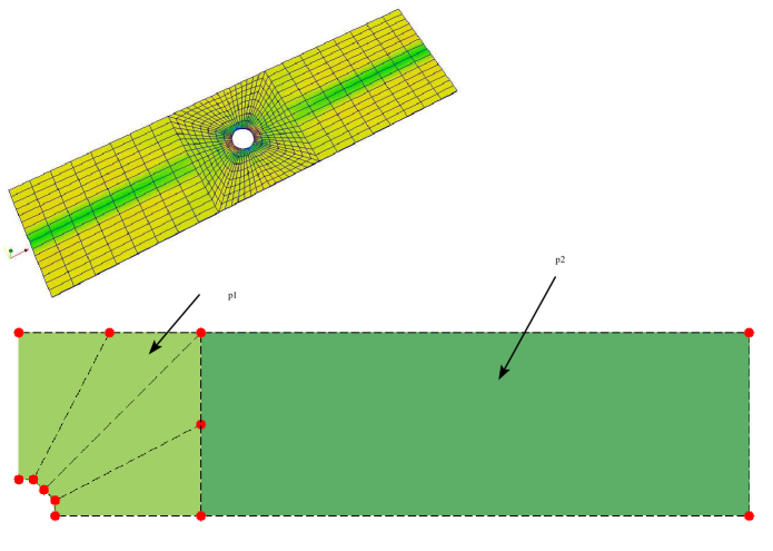
Figure 27: Open hole laminate.

Finally, treatment of doubly curved composite panels is addresses by an example given in Fig. (28). Using a CAD software, the panel is usually a NURBS surface, Fig. (28)–left, a trivariate representation is constructed using the ideas recently reported in [72], Fig. (28)–middle, and FE analyses can be performed, see Fig. (28)–right.

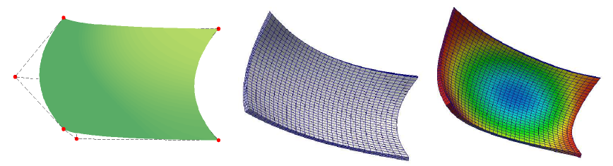
Figure 28: Doubly curved composite laminate: from bi-quadratic NURBS surface to trivariate NURBS solid that is suitable for analysis.

6 Conclusion

An isogeometric computational framework was presented for modeling delamination of two and three dimensional composite laminates. By using the isogeometric concept in which the NURBS representation of the composite laminates is maintained in a finite element environment, it was shown by several examples that the time being spent on preparing analysis suitable models for delamination analyses can be dramatically reduced. This fact is beneficial to designing composite laminates in which various geometry parameters need to be varied. The pre-processing algorithms were explained in details and implemented in MIGFEM–an open source code which is available at https://sourceforge.net/projects/cmcodes/. From the analysis perspective, the ultra smooth high order NURBS basis functions are able to produce highly accurate stress fields which is very important in fracture modeling. The consequence is that relatively coarse meshes (compared to meshes of lower order elements) can be adopted and thus the computational expense is reduced.

Although an elaborated isogeometric computational framework was presented for modeling delaminated composites and several geometry models were addressed, there are certainly a certain number of geometries that has not been treated. One example is three dimensional curved composite panels with cutouts. Possibilities for these problems are trimmed NURBS or T-splines for conforming mesh methods and immersed boundary methods for non-conforming techniques.

References

- [1] T.J.R. Hughes, J.A. Cottrell, and Y. Bazilevs. Isogeometric analysis: CAD, finite elements, NURBS, exact geometry and mesh refinement. Computer Methods in Applied Mechanics and Engineering, 194(39-41):4135–4195, 2005.
- [2] J. A. Cottrell, T. J.R. Hughes, and Y. Bazilevs. Isogeometric Analysis: Toward Integration of CAD and FEA. Wiley, 2009.
- [3] P. Kagan, A. Fischer, and P. Z. Bar-Yoseph. New B-Spline Finite Element approach for geometrical design and mechanical analysis. International Journal for Numerical Methods in Engineering, 41(3):435–458, 1998.
- [4] F. Cirak, M. Ortiz, and P. Schröder. Subdivision surfaces: a new paradigm for thin-shell finite-element analysis. International Journal for Numerical Methods in Engineering, 47(12):2039–2072, 2000.
- [5] İ. Temizer, P. Wriggers, and T.J.R. Hughes. Contact treatment in isogeometric analysis with NURBS. Computer Methods in Applied Mechanics and Engineering, 200(9-12):1100–1112, 2011.
- [6] L. Jia. Isogeometric contact analysis: Geometric basis and formulation for frictionless contact. Computer Methods in Applied Mechanics and Engineering, 200(5-8):726–741, 2011.
- [7] İ. Temizer, P. Wriggers, and T.J.R. Hughes. Three-Dimensional Mortar-Based frictional contact treatment in isogeometric analysis with NURBS. Computer Methods in Applied Mechanics and Engineering, 209–212:115–128, 2012.
- [8] L. De Lorenzis, İ. Temizer, P. Wriggers, and G. Zavarise. A large deformation frictional contact formulation using NURBS-bases isogeometric analysis. International Journal for Numerical Methods in Engineering, 87(13):1278–1300, 2011.
- [9] M.E. Matzen, T. Cichosz, and M. Bischoff. A point to segment contact formulation for isogeometric, NURBS based finite elements. Computer Methods in Applied Mechanics and Engineering, 255:27 – 39, 2013.
- [10] W. A. Wall, M. A. Frenzel, and C. Cyron. Isogeometric structural shape optimization. Computer Methods in Applied Mechanics and Engineering, 197(33-40):2976–2988, 2008.
- [11] N. D. Manh, A. Evgrafov, A. R. Gersborg, and J. Gravesen. Isogeometric shape optimization of vibrating membranes. Computer Methods in Applied Mechanics and Engineering, 200(13-16):1343–1353, 2011.
- [12] X. Qian and O. Sigmund. Isogeometric shape optimization of photonic crystals via Coons patches. Computer Methods in Applied Mechanics and Engineering, 200(25-28):2237–2255, 2011.
- [13] X. Qian. Full analytical sensitivities in NURBS based isogeometric shape optimization. Computer Methods in Applied Mechanics and Engineering, 199(29-32):2059–2071, 2010.
- [14] D.J. Benson, Y. Bazilevs, M.C. Hsu, and T.J.R. Hughes. Isogeometric shell analysis: The Reissner–Mindlin shell. Computer Methods in Applied Mechanics and Engineering, 199(5-8):276–289, 2010.
- [15] J. Kiendl, K.-U. Bletzinger, J. Linhard, and R. Wüchner. Isogeometric shell analysis with Kirchhoff-Love elements. Computer Methods in Applied Mechanics and Engineering, 198(49-52):3902–3914, 2009.
- [16] D.J. Benson, Y. Bazilevs, M.-C. Hsu, and T.J.R. Hughes. A large deformation, rotation-free, isogeometric shell. Computer Methods in Applied Mechanics and Engineering, 200(13-16):1367–1378, 2011.
- [17] L. Beirão da Veiga, A. Buffa, C. Lovadina, M. Martinelli, and G. Sangalli. An isogeometric method for the Reissner-Mindlin plate bending problem. Computer Methods in Applied Mechanics and Engineering, 209–212:45–53, 2012.
- [18] T. K. Uhm and S. K. Youn. T-spline finite element method for the analysis of shell structures. International Journal for Numerical Methods in Engineering, 80(4):507–536, 2009.
- [19] R. Echter, B. Oesterle, and M. Bischoff. A hierarchic family of isogeometric shell finite elements. Computer Methods in Applied Mechanics and Engineering, 254:170 – 180, 2013.
- [20] D.J. Benson, S. Hartmann, Y. Bazilevs, M.-C. Hsu, and T.J.R. Hughes. Blended isogeometric shells. Computer Methods in Applied Mechanics and Engineering, 255:133 – 146, 2013.
- [21] J.A. Cottrell, A. Reali, Y. Bazilevs, and T.J.R. Hughes. Isogeometric analysis of structural vibrations. Computer Methods in Applied Mechanics and Engineering, 195(41-43):5257–5296, 2006.
- [22] T.J.R. Hughes, A. Reali, and G. Sangalli. Duality and unified analysis of discrete approximations in structural dynamics and wave propagation: Comparison of p-method finite elements with k-method NURBS. Computer Methods in Applied Mechanics and Engineering, 197(49–50):4104 – 4124, 2008.
- [23] C. H. Thai, H. Nguyen-Xuan, N. Nguyen-Thanh, T-H. Le, T. Nguyen-Thoi, and T. Rabczuk. Static, free vibration, and buckling analysis of laminated composite Reissner-Mindlin plates using NURBS-based isogeometric approach. International Journal for Numerical Methods in Engineering, 91(6), 2012.
- [24] D. Wang, W. Liu, and H. Zhang. Novel higher order mass matrices for isogeometric structural vibration analysis. Computer Methods in Applied Mechanics and Engineering, pages –, 2013.
- [25] H. Gomez, T.J.R. Hughes, X. Nogueira, and V. M. Calo. Isogeometric analysis of the isothermal Navier-Stokes-Korteweg equations. Computer Methods in Applied Mechanics and Engineering, 199(25-28):1828–1840, 2010.
- [26] P. N. Nielsen, A. R. Gersborg, J. Gravesen, and N. L. Pedersen. Discretizations in isogeometric analysis of Navier-Stokes flow. Computer Methods in Applied Mechanics and Engineering, 200(45-46):3242–3253, 2011.
- [27] Y. Bazilevs and I. Akkerman. Large eddy simulation of turbulent Taylor-Couette flow using isogeometric analysis and the residual-based variational multiscale method. Journal of Computational Physics, 229(9):3402–3414, 2010.
- [28] Y. Bazilevs, V. M. Calo, T. J. R. Hughes, and Y. Zhang. Isogeometric fluid-structure interaction: theory, algorithms, and computations. Computational Mechanics, 43:3–37, 2008.
- [29] Y. Bazilevs, J.R. Gohean, T.J.R. Hughes, R.D. Moser, and Y. Zhang. Patient-specific isogeometric fluid-structure interaction analysis of thoracic aortic blood flow due to implantation of the Jarvik 2000 left ventricular assist device. Computer Methods in Applied Mechanics and Engineering, 198(45-46):3534–3550, 2009.
- [30] H. Gómez, V. M. Calo, Y. Bazilevs, and T.J.R. Hughes. Isogeometric analysis of the Cahn-Hilliard phase-field model. Computer Methods in Applied Mechanics and Engineering, 197(49-50):4333–4352, 2008.
- [31] C. V. Verhoosel, M. A. Scott, T. J. R. Hughes, and R. de Borst. An isogeometric analysis approach to gradient damage models. International Journal for Numerical Methods in Engineering, 86(1):115–134, 2011.
- [32] P. Fischer, M. Klassen, J. Mergheim, P. Steinmann, and R. Müller. Isogeometric analysis of 2D gradient elasticity. Computational Mechanics, 47:325–334, 2010.
- [33] A. Masud and R. Kannan. B-splines and NURBS based finite element methods for Kohn-Sham equations. Computer Methods in Applied Mechanics and Engineering, 241-244:112 – 127, 2012.
- [34] V. P. Nguyen, R. Simpson, S.P.A. Bordas, and T. Rabczuk. Isogeometric analysis: An overview and computer implementation aspects. Advances in Engineering Softwares, pages –, 2013. submitted.
- [35] E. De Luycker, D. J. Benson, T. Belytschko, Y. Bazilevs, and M. C. Hsu. X-FEM in isogeometric analysis for linear fracture mechanics. International Journal for Numerical Methods in Engineering, 87(6):541–565, 2011.
- [36] S. S. Ghorashi, N. Valizadeh, and S. Mohammadi. Extended isogeometric analysis for simulation of stationary and propagating cracks. International Journal for Numerical Methods in Engineering, 89(9):1069–1101, 2012.
- [37] A. Tambat and G. Subbarayan. Isogeometric enriched field approximations. Computer Methods in Applied Mechanics and Engineering, 245–246:1 – 21, 2012.
- [38] M. J. Borden, C. V. Verhoosel, M. A. Scott, T. J.R. Hughes, and C. M. Landis. A phase-field description of dynamic brittle fracture. Computer Methods in Applied Mechanics and Engineering, 217–220:77 – 95, 2012.
- [39] C. V. Verhoosel, M. A. Scott, R. de Borst, and T. J. R. Hughes. An isogeometric approach to cohesive zone modeling. International Journal for Numerical Methods in Engineering, 87(1‐5):336–360, 2011.
- [40] O. Allix, P. Ladevèze, and A. Corigliano. Damage analysis of interlaminar fracture specimens. Composite Structures, 31(1):61 – 74, 1995.
- [41] J.C.J. Schellekens and R. De Borst. A non-linear finite element approach for the analysis of mode-I free edge delamination in composites. International Journal of Solids and Structures, 30(9):1239 – 1253, 1993.
- [42] G. Alfano and M. A. Crisfield. Finite element interface models for the delamination analysis of laminated composites: mechanical and computational issues. International Journal for Numerical Methods in Engineering, 50(7):1701–1736, 2001.
- [43] R Krueger and T.K O’Brien. A shell/3D modeling technique for the analysis of delaminated composite laminates. Composites Part A: Applied Science and Manufacturing, 32(1):25 – 44, 2001.
- [44] E. F. Rybicki and M. F. Kanninen. A finite element calculation of stress intensity factors by a modified crack closure integral. Engineering Fracture Mechanics, 9:931–938, 1977.
- [45] R. Krueger. The virtual crack closure technique: History, approach and applications. Technical report, NASA. NASA/CR-2002-211628, ICASE Report No. 2002-10, 2002.
- [46] I. Guiamatsia, B.G. Falzon, G.A.O. Davies, and L. Iannucci. Element-free galerkin modelling of composite damage. Composites Science and Technology, 69(15–16):2640 – 2648, 2009.
- [47] M. Samimi, J.A.W. van Dommelen, and M.G.D. Geers. A self-adaptive finite element approach for simulation of mixed-mode delamination using cohesive zone models. Engineering Fracture Mechanics, 78(10):2202 – 2219, 2011.
- [48] I. Guiamatsia, J.K. Ankersen, G.A.O. Davies, and L. Iannucci. Decohesion finite element with enriched basis functions for delamination. Composites Science and Technology, 69(15–16):2616 – 2624, 2009.
- [49] N. Moës, J. Dolbow, and T. Belytschko. A finite element method for crack growth without remeshing. International Journal for Numerical Methods in Engineering, 46(1):131–150, 1999.
- [50] J. J. C. Remmers, G. N. Wells, and R. Borst. A solid-like shell element allowing for arbitrary delaminations. International Journal for Numerical Methods in Engineering, 58(13):2013–2040, 2003.
- [51] T. Nagashima and H. Suemasu. Stress analyses of composite laminate with delamination using X-FEM. International Journal of Computational Methods, 03(04):521–543, 2006.
- [52] J.L. Curiel Sosa and N. Karapurath. Delamination modelling of GLARE using the extended finite element method. Composites Science and Technology, 72(7):788 – 791, 2012.
- [53] V. P. Nguyen and H. Nguyen-Xuan. High-order B-splines based finite elements for delamination analysis of laminated composites. Composite Structures, 102:261–275, 2013.
- [54] B. Gözlüklü and D. Coker. Modeling of the dynamic delamination of L-shaped unidirectional laminated composites. Composite Structures, 94(4):1430 – 1442, 2012.
- [55] G. Wimmer and H.E. Pettermann. A semi-analytical model for the simulation of delamination in laminated composites. Composites Science and Technology, 68(12):2332 – 2339, 2008.
- [56] L. A. Piegl and W. Tiller. The NURBS Book. Springer, 1996.
- [57] Rhino. CAD modeling and design toolkit. www.rhino3d.com.
- [58] M. J. Borden, M. A. Scott, J. A. Evans, and T. J. R. Hughes. Isogeometric finite element data structures based on Bézier extraction of NURBS. International Journal for Numerical Methods in Engineering, 87(1‐5):15–47, 2011.
- [59] M. A. Scott, M. J. Borden, C. V. Verhoosel, T. W. Sederberg, and T. J. R. Hughes. Isogeometric finite element data structures based on Bézier extraction of T-splines. International Journal for Numerical Methods in Engineering, 88(2):126–156, 2011.
- [60] V. P. Nguyen. On some practical aspects of fracture modelling using interface elements. Technical report, Delft University of Technology, The Netherlands, 2009. http://www.academia.edu/1188763/interface-mesh-generator.
- [61] P. P. Camanho, C. G. Davila, and M. F. de Moura. Numerical simulation of mixed-mode progressive delamination in composite materials. Journal of Composite Materials, 37(16):1415–1438, 2003.
- [62] A. Turon, P.P. Camanho, J. Costa, and C.G. Dávila. A damage model for the simulation of delamination in advanced composites under variable-mode loading. Mechanics of Materials, 38(11):1072 – 1089, 2006.
- [63] M.L. Benzeggagh and M. Kenane. Measurement of mixed-mode delamination fracture toughness of unidirectional glass/epoxy composites with mixed-mode bending apparatus. Composites Science and Technology, 56(4):439 – 449, 1996.
- [64] F.P. van der Meer and L.J. Sluys. Mesh-independent modeling of both distributed and discrete matrix cracking in interaction with delamination in composites. Engineering Fracture Mechanics, 77(4):719 – 735, 2010.
- [65] F.P. van der Meer. Mesolevel modeling of failure in composite laminates: Constitutive, kinematic and algorithmic aspects. Archives of Computational Methods in Engineering, 19(3):381–425, 2012.
- [66] M. A. Gutiérrez. Energy release control for numerical simulations of failure in quasi-brittle solids. Communications in Numerical Methods in Engineering, 20(1):19–29, 2004.
- [67] C. V. Verhoosel, J. J. C. Remmers, and M. A. Gutiérrez. A dissipation-based arc-length method for robust simulation of brittle and ductile failure. International Journal for Numerical Methods in Engineering, 77(9):1290–1321, 2009.
- [68] E. J. Lingen and M. Stroeven. Jem/Jive-a C++ numerical toolkit for solving partial differential equations. http://www.habanera.nl/.
- [69] Y. Mi, M. A. Crisfield, G. A. O. Davies, and H. B. Hellweg. Progressive delamination using interface elements. Journal of Composite Materials, 32(14):1246–1272, 1998.
- [70] G. Kress, R. Roos, M. Barbezat, C. Dransfeld, and P. Ermanni. Model for interlaminar normal stress in singly curved laminates. Composite Structures, 69(4):458 – 469, 2005.
- [71] R. Roos, G. Kress, M. Barbezat, and P. Ermanni. Enhanced model for interlaminar normal stress in singly curved laminates. Composite Structures, 80(3):327 – 333, 2007.
- [72] V. P. Nguyen, P. Kerfriden, S.P.A. Bordas, and T. Rabczuk. An integrated design-analysis framework for three dimensional composite panels. Computer Aided Design, 2013. submitted.
- [73] Y. Bazilevs, V.M. Calo, J.A. Cottrell, J.A. Evans, T.J.R. Hughes, S. Lipton, M.A. Scott, and T.W. Sederberg. Isogeometric analysis using T-splines. Computer Methods in Applied Mechanics and Engineering, 199(5-8):229–263, 2010.