$d$-wave superconductivity and its coexistence with antiferromagnetism in $t$–$J$–$U$ model: Statistically consistent Gutzwiller approach

Abstract

We discuss the coexistence of antiferromagnetism and $d$-wave superconductivity within the so-called statistically-consistent Gutzwiller approximation (SGA) applied to the $t$–$J$–$U$ model. In this approach, the averages calculated in a self-consistent manner coincide with those determined variationally. Such consistency is not guaranteed within the standard renormalized mean field theory. With the help of SGA, we show that for the typical value $J/|t|=1/3$, coexistence of antiferromagnetism (AF) and superconductivity (SC) appears only for $U/|t|>10.6$ and in a very narrow range of doping $(\delta\lesssim 0.006)$ in the vicinity of the Mott insulating state, in contrast to some previous reports. In the coexistent AF+SC phase, a staggered spin-triplet component of the superconducting gap appears also naturally; its value is very small.

I Introduction: rationale for $t$–$J$–$U$ model

High-temperature superconductivity in cuprates is often described within the effective $t$–$J$ modelSpałek and Oleś (1977); *ChaoSpalekOles1977-JPhysC.10.L271; Spałek (2007) (for a preliminary treatment of the topic c.f. also Ref. Anderson, 1988). The model justifies a number of experimental results, such as superconductivity’s dome-like shape on doping-temperature phase diagram,Dagotto (1994) non-Fermi-liquid behavior of the normal state for underdoped and optimally doped systems,Sarker et al. (1994); *Sarker2010-PRB.82.014504; Johnson et al. (2001); Lee et al. (2006) the disappearance of the pairing gap magnitude in the antiferromagnetic state (albeit only at the doping $\delta=0$),Lee et al. (2006); Imada et al. (1998) and the doping dependence of the photoemission spectrum in the antinodal direction.Damascelli et al. (2003); Tanaka et al. (206) All of these features represent an attractive starting point for further analysis (cf. Ref. Scalapino, 2012).

In the effective $t$–$J$ model, the value of the kinetic exchange integral $J_{ij}$ does not necessarily coincide with the value $J_{ij}=4t_{ij}^{2}/U$ obtained perturbationally from the Hubbard model.Spałek (2007) Instead, it expresses an effective coupling between the copper spins in mixed copper-oxygen $3d$–$2p$ holes.Zhang and Rice (1988) Therefore, one may say that the values of the hopping integral $t_{ij}$ and that of antiferromagnetic exchange $J_{ij}$ in that model are practically independent. Typically, the ratio $|t|/J\approx 3$ is taken and corresponds to the value $U/(8|t|)=1.5$ in the context of the two-dimensional Hubbard model. However, after introducing the bare bandwidth $W=8|t|$ in the tight-binding approximation for a square lattice, we obtain the ratio $U/W=1.5$, which is not sufficiently large for the transformation of the original Hubbard model into the $t$–$J$ model to be valid in the low order. In that situation, we are, strictly speaking not within the strong correlation limit $U/W\gg 1$, in which the $t$–$J$ model was originally derived.Spałek and Oleś (1977); *ChaoSpalekOles1977-JPhysC.10.L271; Spałek (2007)

In order to account properly for the strong electronic correlations (the bare Hubbard parameter $U$ for Cu²⁺ ion is $8\mbox{-}10\ \mbox{eV}\gg W\approx 2-3\ \mbox{eV}$), we can add the Hubbard term $U\sum_{i}\hat{n}_{i\uparrow}\hat{n}_{i\downarrow}$ to the $t$–$J$ model. In this manner, we consider the exchange integral $J_{ij}$ in this still-effective single-band model as coming from the full superexchange involving the oxygen ions rather than from the effective kinetic exchange only (for critical overview c.f. Ref. Zaanen and Sawatzky, 1990). This argument may be regarded as one of the justifications for introducing the $t$–$J$–$U$ model, first used by Daul,Daul et al. (2000) Basu,Basu et al. (2001) and ZhangZhang (2003) (cf. Ref. Xiang et al., 2009, where comprehensive justification of the $t$–$J$–$U$ is provided).

There is an additional reason for the $t$–$J$–$U$ model applicability to the cuprates. Namely, in the starting, bare configuration of CuO${}_{2}^{2-}$ structural unit, the hybridization between the antibonding $2p_{\sigma}$ states due to oxygen and one-hole $(3d^{9})$ states due to Cu is strong, with the hybridization matrix element $|V_{\langle im\rangle}|\sim 1.5$ eV. Therefore, the hybridization contribution to the hole state itinerancy, at least on the single-particle level, is essential and hence the effective $d$–$d$ (Hubbard) interaction is substantially reduced. In effect, we may safely assume that $U\gtrsim W$ instead $U\gg W$. In this manner, the basic simplicity of the single-band model is preserved, as it provides not only the description of the strongly correlated metallic state close to the Mott insulating limit, but also reduces to the correct limit of the Heisenberg magnet of spin $1/2$ with strong antiferromagnetic exchange integral $J\approx 0.1$ eV in the absence of holes (the Mott-Hubbard insulating state). Last but not least, within the present model we can study the limit $U\rightarrow\infty$ and compare explicitly the results with those of canonical $t$–$J$ model.

Antiferromagnetism (AF) and superconductivity (SC) can coexist in the electron doped cuprates,Yu et al. (2007); Armitage et al. (2010) but in the hole-doped cuprates the two phases are usually separated (cf. e.g. the review of DagottoDagotto (1994)). However, in the late 1990s, reports of a possible coexistence in the cuprates appeared, first vague (cf. Ref. Kimura et al., 1999 (La_2-xSr_xCu_1-yZn_yO₄)), then more convincing (cf. e.g. Ref. Lee et al., 1999 (La₂CuO_4+y), Ref. Sidis et al., 2001 (Y​Ba₂Cu₃O_6.5) or Ref. Hodges et al., 2002 (YBa₂(Cu_0.987Co_0.013)₃O_y+δ)). Other systems, where the coexistence has been reported, are organic superconductors,Kawamoto et al. (2008) heavy-fermions systems,Mathur et al. (1998) iron-based superconductors such as Ba(Fe_1-xRu_x)₂As₂ (Ref. Ma et al., 2012), Ba_0.77K_0.23Fe₂As₂ (Ref. Li et al., 2012), Ba(Fe_1-xCo_x)₂As₂ (Ref. Marsik et al., 2010; Bernhard et al., 2012), as well as graphene bilayer systems (cf. Ref. Milovanović and Predin, 2012).

Our purpose is to undertake a detailed analysis of the paired (SC) state within the $t$–$J$–$U$ model and its coexistence with the two-sublattice antiferromagnetism in two dimensions. Detailed studies of the $t$–$J$–$U$ model have been carried out by Zhang,Zhang (2003) Gan,Gan et al. (2005a, b) and BernevigBernevig et al. (2003) who described a transition from gossamerLaughlin (2006) and $d$-waveVan Harlingen (1995); Tsuei and Kirtley (2000) superconductivity to the Mott insulator. However, the existence of AF order was not considered in those studies. Some attempts to include AF order were made by YuanYuan et al. (2005) and Heiselberg,Heiselberg (2009) and very recently by VooVoo (2011) and Liu,Liu et al. (2012) but in all those works one can question the authors’ approach. Specifically, the equations used do not guarantee self-consistency, i.e. the mean-field averages introduced in a self-consistent manner do not match those determined variationally.Jędrak et al. (2010) We show that the above problem that appears in the Renormalized Mean Field Theory (RMFT) formulation, can be overcome by introducing constraints that ensure the statistical consistency between the two above ways of determining mean-field values. This is the principal concept of our statistically consistent Gutzwiller approach (SGA).Jędrak and Spałek (2010); Jędrak (2011)

Using SGA we obtain that AF phase is stable only in the presence of SC in a very narrow region close to the Mott-Hubbard insulating state, corresponding to the half-filled (undoped) situation. Additionally, in this AF-SC coexisting phase, a small staggered spin-triplet component of the superconducting gap appears naturally, in addition to the predominant spin-singlet component.

The structure of the paper is as follows. In Sec. II, we define the model and provide definitions of the mean-field parameters. In Sec. III, we introduce the constraints with the corresponding Lagrange multipliers to guarantee the consistency of the self-consistent and the variational procedures of determining the mean-field parameters. The full minimization procedure is also outlined there. In Sec. IV, we discuss the numerical results, as well as provide the values of the introduced Lagrange multipliers. In Sec. V, we summarize our results and compare them with those of other studies. In Appendix A, we discuss the general form of the hopping amplitude and the superconducting gap, as well as some details of the analytic calculations required to determine the ground state energy. In Appendixes B and C, we show some details of our calculations. In Appendix D, we present an alternative and equivalent procedure of introducing the Lagrange multipliers to that presented in the main text. In Appendix E, we list representative values of the parameters calculated for different phases.

II $t$–$J$–$U$ Model and effective single-particle Hamiltonian

We start from the $t$–$J$–$U$ model as represented by the HamiltonianZhang (2003); Gan et al. (2005a, b)

$$\mathcal{\mathcal{\hat{H}}}=\ t\sum_{\left\langle i\,j\right\rangle,\,\sigma}\left(\hat{c}^{\dagger}_{i\sigma}\hat{c}_{j\sigma}+\text{H.c.}\right)+J\sum_{\left\langle i\,j\right\rangle}{\bf\hat{S}}_{i}\cdot{\bf\hat{S}}_{j}+U\sum_{i}\hat{n}_{i\uparrow}\hat{n}_{i\downarrow},\\$$ (1)

where: $\sum_{\left\langle i\,j\right\rangle}$ denotes the summation over the nearest neighboring sites, $t$ is the nearest-neighbor hopping integral, $J$ is the effective antiferromagnetic exchange integral, ${\bf\hat{S}}_{i}$ is the spin operator in the fermion representation, and $U$ is the on-site Coulomb repulsion magnitude.

One methodological remark is in place here. Usually, when starting from the Hubbard or $t$–$J$ models and discussing subsequently the correlated states and phases, one neglects the intersite repulsive Coulomb interaction $\sim\ K\sum_{\langle ij\rangle}\hat{n}_{i}\hat{n}_{j}$, where $\hat{n}_{i}=\sum_{\sigma}\hat{n}_{i\sigma}$ is the number of particles on site $i$. In the strong-correlation limit $U\gg W$ the corresponding transformation to the effective $t$-$J$ model providesSpałek (2007) the effective exchange integral $J_{ij}=4t_{ij}^{2}/(U-K)$, and since $K\sim U/3$, we have a strong enhancement ($\sim 30\%$) of the kinetic exchange integral. Strictly speaking, the contribution $\sim K$ should be then also added to the effective Hamiltonian (1). However, this term has been neglected, as well as the similar contribution $\sim(J/4)\sum_{\langle ij\rangle}\hat{n}_{i}\hat{n}_{j}$ appearing in the full Dirac exchange operator Spałek (2007), since we assume that the physically meaningful regime is that with $U\gtrsim W\gg K$ so that any charge-density wave instability is irrelevant in this limit.

We study properties of the above Hamiltonian using the Gutzwiller variational approach,Gutzwiller (1963); *Gutzwiller1965-pr in which the trial wave function has the formLaughlin (2006); Yuan et al. (2005); Heiselberg (2009) $|\Psi\rangle=\hat{P}_{G}|\Psi_{0}\rangle$, where $\hat{P}_{G}$ is an operator specifying explicitly the configurations with double on-site occupancies, and $|\Psi_{0}\rangle$ is an eigenstate of a single-particle Hamiltonian (to be defined later). Since the correlated state $|\Psi\rangle$ is related to $|\Psi_{0}\rangle$, the average value of the Hamiltonian $\mathcal{\mathcal{\hat{H}}}$ can be expressed as

$$\frac{\langle\Psi|\mathcal{\hat{H}}|\Psi\rangle}{\langle\Psi|\Psi\rangle}=\frac{\langle\Psi_{0}|\hat{P}_{G}\mathcal{\hat{H}}\hat{P}_{G}|\Psi_{0}\rangle}{\langle\Psi_{0}|\hat{P}_{G}^{2}|\Psi_{0}\rangle}\approx\langle\Psi_{0}|\mathcal{\hat{H}}_{\text{\it eff}}|\Psi_{0}\rangle\equiv\langle\mathcal{\hat{H}}_{\text{\it eff}}\rangle_{0},$$ (2)

where $\langle\ldots\rangle_{0}$ means the average evaluated with respect to $|\Psi_{0}\rangle$, andZhang (2003); Gan et al. (2005a, b); Yuan et al. (2005); Heiselberg (2009)

$$\mathcal{\mathcal{\hat{H}}}_{\mathit{eff}}=\ g_{t}t\sum_{\left\langle i\,j\right\rangle,\,\sigma}\left(\hat{c}^{\dagger}_{i\sigma}\hat{c}_{j\sigma}+\text{H.c.}\right)+g_{s}J\sum_{\left\langle i\,j\right\rangle}{\bf\hat{S}}_{i}\cdot{\bf\hat{S}}_{j}+Ud^{2}\\$$ (3)

is the effective Hamiltonian resulting from the Gutzwiller approximationGutzwiller (1963); *Gutzwiller1965-pr (GA). In the above formula, ${d^{2}\equiv\left\langle\hat{n}_{i\uparrow}\hat{n}_{i\downarrow}\right\rangle_{0}}$ is the double-occupancy probability, $g_{t}$ and $g_{s}$ are the so-called Gutzwiller renormalization factors determined by the statistical counting of configuration with given $Nd^{2}$, $Nw$ and $Nr$. (cf. Refs. Ogawa et al., 1975; Zhang et al., 1988)

$$g_{t} = \frac{n-2d^{2}}{n-2rw}\left(\sqrt{\frac{(1-w)(1-n+d^{2})}{1-r}}\right.+\left.\sqrt{\frac{wd^{2}}{r}}\right)$$ (4a)

$$\times\left(\sqrt{\frac{(1-r)(1-n+d^{2})}{1-w}}+\sqrt{\frac{rd^{2}}{w}}\right),$$

$$g_{s} = \left(\frac{n-2d^{2}}{n-2rw}\right)^{2},$$ (4b)

where $n$ is the average number of electrons (occupancy) per site. To discuss AF order, the lattice is divided into two interpenetrating sublattices: $A$, where the majority of spins are oriented $\uparrow$, and $B$, where the majority of spins are oriented $\downarrow$. For sublattice $A$, $r\equiv\langle\hat{n}_{i\uparrow}\rangle=\frac{1}{2}\left(n+m_{AF}\right)$ and $w\equiv\langle\hat{n}_{i\downarrow}\rangle=\frac{1}{2}\left(n-m_{AF}\right)$, where $m_{AF}$ is the antiferromagnetic (staggered) spin polarization per site. For sublattice $B$, the definitions of $w$ and $r$ are interchanged. Note, that the Gutzwiller factor (4b) has the same form for both $\frac{1}{2}\left(\hat{S}^{x}_{i}\hat{S}^{y}_{j}+\hat{S}^{x}_{i}\hat{S}^{y}_{j}\right)$ and $\hat{S}^{z}_{i}\hat{S}^{z}_{j}$ parts of ${\bf\hat{S}}_{i}\cdot{\bf\hat{S}}_{j}$. In a refined approach, two distinct Gutzwiller factors $g_{s}^{xy}$ and $g_{x}^{z}$ may be considered (cf. Ref. Himeda and Ogata, 1999). However, in this paper it is assumed that $g_{s}^{xy}=g_{x}^{z}\equiv g_{s}$, which is broadly accepted (see e.g. Refs. Zhang, 2003; Gan et al., 2005a, b; Yuan et al., 2005; Heiselberg, 2009). The reason is that the spin-singlet paired state is spin-rotationally invariant and in the case of coexistent antiferromagnetic state we limit ourselves to the mean-field-approach paradigm with the resulting Néel state.

In order to evaluate $\langle\mathcal{\hat{H}}_{\text{\it eff}}\rangle_{0}$ we define the average number of electrons per site with spin $\sigma$ as

$$n_{i\sigma}\equiv\langle\hat{c}^{\dagger}_{i\sigma}\hat{c}_{i\sigma}\rangle_{0}=\frac{1}{2}\left(n+\sigma\,e^{i{\bf Q}\cdot{\bf R}_{i}}\,m_{AF}\right),$$ (5)

with ${\bf Q}\equiv(\pi,\,\pi)$, and with ${\bf R}_{i}$ denoting position vector of site $i$ and the following bare (nonrenormalized) quantities: the hopping amplitude for the nearest neighbors $\langle i,j\rangle$ as

$$\chi_{ij\sigma}\equiv\langle\hat{c}^{\dagger}_{i\sigma}\hat{c}_{j\sigma}\rangle_{0}=\chi_{AB},$$ (6)

and the pairing order parameter in real space in the form

$$\Delta_{ij\sigma}\equiv\langle\hat{c}_{i\sigma}\hat{c}_{j\bar{\sigma}}\rangle_{0}\equiv-\tau_{ij}\left(\sigma\Delta_{S}+e^{i{\bf Q}\cdot{\bf R}_{i}}\Delta_{T}\right),$$ (7)

where $\tau_{ij}\equiv 1$ for $j=i\pm\hat{x}$ and ${\tau_{ij}\equiv-1}$ for $j=i\pm\hat{y}$ (in order to ensure the $d$-wave symmetry). In consequence, the spin-singlet $(\Delta_{S})$ and the spin-triplet $(\Delta_{T})$ components of the gap are defined as

$$\tau_{ij}\Delta_{S} = \frac{1}{4}\left(\left\langle\hat{c}_{j\in B\,\downarrow}\hat{c}_{i\in A\uparrow}\right\rangle_{0}+\left\langle\hat{c}_{i\in A\,\downarrow}\hat{c}_{j\in B\uparrow}\right\rangle_{0}+\mbox{H.c.}\right)$$ (8a)

$$= \frac{1}{4}\tau_{ij}\left(\Delta_{A}+\Delta_{B}+\mbox{H.c.}\right),$$

$$\tau_{ij}\Delta_{T} = \frac{1}{4}\left(\left\langle\hat{c}_{j\in B\,\downarrow}\hat{c}_{i\in A\uparrow}\right\rangle_{0}-\left\langle\hat{c}_{i\in A\,\downarrow}\hat{c}_{j\in B\uparrow}\right\rangle_{0}+\mbox{H.c.}\right)$$ (8b)

$$= \frac{1}{4}\tau_{ij}\left(\Delta_{A}-\Delta_{B}+\mbox{H.c.}\right).$$

In some works (e.g. in Refs. Yuan et al., 2005; Heiselberg, 2009) the triplet component is disregarded. However, since $\Delta_{A}$ represents an average pairing for majority spins on nearest neighboring sites and $\Delta_{B}$ an average pairing of minority spins (when AF order is present, cf. Fig. 1), the real part of $\Delta_{A}$ and $\Delta_{B}$ might be different (cf. also the work of TsonisTsonis et al. (2008) and AperisAperis et al. (2010) regarding the inadequacy of a single-component order parameter to describe the SC phase). Therefore, in this paper, this more comprehensive structure is introduced. Nonetheless, in order to evaluate the significance of introducing the triplet term for the SC gap, the results are compared also with those obtained for the case when $\Delta_{T}$ is set to zero.

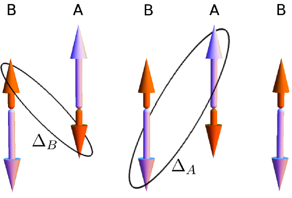
Figure 1: (Color online) Schematic representation of the difference between the pairing parameters for the majority-spin electrons (large arrows) and the minority-spin electrons (small arrows) in the two-sublattice system with AF order. Since for $m_{AF}\neq 0$ there may be that the real part of $\Delta_{A}$ and $\Delta_{B}$ might be different, and a spin-triplet component of the superconducting order has to be considered [cf. Eq. (8b)].

Applying the Wick’s theorem to the Eq. (2), the expectation value $\left\langle\mathcal{\mathcal{\hat{H}}}_{\mathit{eff}}\right\rangle_{0}\equiv W$ can be obtained in the form (see Appendix A for details)

$$\frac{W}{\Lambda}=8g_{t}t\chi_{AB}+Ud^{2}-g_{s}J\left(\frac{1}{2}m_{AF}^{2}+3\chi_{AB}^{2}+3\Delta_{S}^{2}-\Delta_{T}^{2}\right),$$ (9)

where $\Lambda$ is the number of atomic sites in the system. Note that the total energy of this correlated system is composed of three interdependent parts: (i) the renormalized hopping energy $\sim tg_{t}\chi_{AB}<0$, (ii) the correlation energy $Ud^{2}>0$, and (iii) the exchange contribution $\sim g_{s}J$ lowering both the energies of AF and SC states. This balance of physical energies will be amended next by the constraints introducing the statistical consistency into this mean-field system to guarantee that the self-consistent and the variational procedures will lead to the same single-particle states (this is the so-called Bogoliubov principle for the optimal single-particle states))

To summarize, the process of derivation of the effective single-particle Hamiltonian (3) is fully justified by its definition (2) which involves an averaging procedure over an uncorrelated state $|\Psi_{0}\rangle$. This state is selected implicitly. In general, it is the state with broken symmetry, i.e. with nonzero values of $m_{AF}$, $\Delta_{S}$, and $\Delta_{T}$. In other words, $|\Psi_{0}\rangle$ is defined through the values of order parameters to be determined either self-consistently or variationally. This is the usual procedure proposed originally by BogoliubovBogoliubov (1958a); *Bogoliubov1958-USSR; *BogoliubovTolmachev1958 in his version of BCS theory and by SlaterSlater (1951) in the theory of itinerant antiferromagnetism. Here their simple version of mean theory becomes more sophisticated, since the renormalization factors contain also the order parameters and in a singular formal form. This last feature leads to basic formal changes in formulation of the renormalized mean-field theory, as discussed next.

III Quasiparticle states and minimization procedure for the ground state

Following Refs. Jędrak and Spałek, 2010; Jędrak, 2011; Jędrak et al., 2010; Kaczmarczyk and Spałek, 2011; Kaczmarczyk, 2011, we write the mean-field grand Hamiltonian in the form

$$\allowdisplaybreaks\hat{K}\equiv W-\sum_{\left\langle i\,j\right\rangle,\,\sigma}\left(\lambda_{ij\sigma}^{\chi}\left(\hat{c}_{i\sigma}^{\dagger}\hat{c}_{j\sigma}-\chi_{ij\sigma}\right)+\text{H.c.}\right)\\ -\sum_{\left\langle i\,j\right\rangle,\,\sigma}\left(\lambda_{ij\sigma}^{\Delta}\left(\hat{c}_{i\sigma}\hat{c}_{j\bar{\sigma}}-\Delta_{ij\sigma}\right)+\text{H.c.}\right)\\ -\sum_{i\sigma}\left(\lambda_{i\sigma}^{n}\left(\hat{n}_{i\sigma}-n_{i\sigma}\right)\right)-\mu\sum_{i\sigma}\hat{n}_{i\sigma},$$ (10)

where $\mu$ is the chemical potential, and the Lagrange multipliers $\{\lambda\}$ are introduced for each operator whose average appears in $W$ [Eq. (9)]. The Lagrange multipliers can be interpreted as the correlation-induced effective fields. We should underline, that the additional terms guarantee that the averages calculated in a self-consistent manner coincide with those determined from variational minimization principle of the appropriate free- or ground-state energy functional. Due to the dependence of the renormalization factors on the mean-field values, the two ways of their calculation do differ, but the introduced constraints ensure their equality. In this manner, as said above, the approach is explicitly in agreement with the Bogoliubov theorem that the single-particle approach represents the optimal formulation from the principle of maximal-entropy point of viewJędrak and Spałek (2010); Jędrak (2011). Also, the fields $\{\lambda\}$ are assumed to have the same symmetry as the broken-symmetry states, to which they are applied [cf. Eqs. (5), (6), and (7)]. Namely,

$$\lambda^{n}_{i\sigma} = \frac{1}{2}\left(\lambda_{n}+\sigma e^{i{\bf Q}\cdot{\bf r}_{i}}\lambda_{m}\right),$$ (11a)

$$\lambda^{\chi}_{ij\sigma} = \lambda_{\chi},$$ (11b)

$$\lambda^{\Delta}_{ij\sigma} = -\tau_{ij}\left(\sigma\lambda_{\Delta_{S}}+e^{i{\bf Q}\cdot{\bf r}_{i}}\lambda_{\Delta_{T}}\right).$$ (11c)

To solve Hamiltonian (10), space Fourier transformation is performed first. Then, the Hamiltonian is diagonalized and yields four branches of eigenvalues (details of the calculations are presented in Appendix B). Next, we define the generalized grand potential functional at temperature $T>0$ as given by

$$\mathcal{F}=-\frac{1}{\beta}\ln{\mathcal{Z}},\hskip 6.0pt\mbox{with}\hskip 6.0pt\mathcal{Z}=\mathrm{Tr}\left(e^{-\beta\hat{K}}\right),$$ (12)

with $\beta\equiv 1/k_{B}T$. Explicitly, $\mathcal{F}$ then has the following form [cf. Eq. (36) in Appendix B]:

$$\mathcal{F}/\Lambda=8g_{t}t\chi_{AB}-g_{s}J\left(\frac{1}{2}m_{AF}^{2}+3\chi_{AB}^{2}+3\Delta_{S}^{2}-\Delta_{T}^{2}\right)\\ +\frac{1}{2}\lambda_{n}(n-1)+\frac{1}{2}\lambda_{m}m_{AF}+8\left(\lambda_{\chi}\chi_{AB}+\lambda_{\Delta_{S}}\Delta_{S}+\lambda_{\Delta_{T}}\Delta_{T}\right)\\ -\frac{1}{\Lambda\beta}\sum_{l,{\bf k}}\ln(1+e^{-\beta E_{l{\bf k}}})+Ud^{2}-\mu.$$ (13)

The necessary conditions for the minimum of $\mathcal{F}$ subject to all constraints are

$$\frac{\partial\mathcal{F}}{\partial\vec{A}}=0,\hskip 6.0pt\hskip 6.0pt\frac{\partial\mathcal{F}}{\partial\vec{\lambda}}=0,\hskip 6.0pt\mbox{and}\hskip 6.0pt\frac{\partial\mathcal{F}}{\partial d}=0,$$ (14)

where the five mean-field parameters are labeled collectively as $\vec{A}$, and the Lagrange multipliers as $\vec{\lambda}$ [the full form of Eqs. (14) is presented in Appendix C]. Note that five above equations ($\partial\mathcal{F}/\partial\vec{A}=0$) can be easily eliminated, reducing the system of algebraic equations to be solved (cf. Appendix C and discussion in Appendix D).

One should note one nontrivial methodological feature of the approach contained in the grand Hamiltonian (10). namely, the effective Hamiltonian (3) appears in it in the form of expectation value $W$ [cf. Eq. (9)], whereas the constraints appear in Eq. (10) in the explicite operator form. This is a nonstandard mean-field version of approach. The correspondence to and main difference with the standard renormalized mean-field approach is discussed in Appendix D.

As we are interested in the ground-state properties (${T=0}$), we take the ${T\rightarrow 0}$ limit. We have checked that taking $\beta^{-1}=k_{B}T=0.002\,|t|$ is sufficient for practical purposes.

IV Results: Phase diagram and microscopic characteristics

The stable phase is determined by the solution which has the lowest physical free energy defined as minimal value of

$$F=\mathcal{F}_{0}+\mu\Lambda n,$$ (15)

where $\mathcal{F}_{0}$ denotes the value of $\mathcal{F}$ obtained at the minimum [cf. conditions (14)].

The minimum of $\mathcal{F}$ was obtained numerically using GNU Scientific Library (GSL),Galassi et al. (2009) and unless stated otherwise, all calculations were made for $t=-1$, $J=|t|/3$, $\beta|t|=500$ on a two-dimensional square lattice of size $\Lambda=512\times 512$ with periodic boundary conditions.

A representative phase diagram on the Coulomb repulsion $U$ – hole doping $\delta$ plane is exhibited in Fig. 2. We find three stable phases: SC, AF and phase with coexisting SC and AF order (labeled collectively as AF+SC). The pure AF stable phase is found only for $\delta\equiv 1-n=0$ and $U/|t|>10.6$. The region where the AF+SC appears is limited to a very close proximity to the Mott insulating state (hole-doping range ${\delta\in(0,\,0.006)}$). Our results differ significantly from previous studies (cf., e.q., Refs. Yuan et al., 2005; Heiselberg, 2009; Liu et al., 2012), where a much wider coexistence region was reported (dashed line in Fig. 2). The previous results were an effect of the non-statistically-consisted RMFT approach used, as also is explained below. Using our method, such a consistency is achieved, and as a result a much narrower coexistence regime appears. It squares with recent experimental studies, where the region of AF+SC was reported to be narrow {cf. e.g. BernhardBernhard et al. (2012) [study of Ba(Fe_1-xCo_x)₂As₂], where the coexistence region is not wider than $0.02$ (of the hole doping range)}.

For further analysis we restrict ourselves to $U/|t|=12$, as marked by the dashed vertical line in Fig. 2. In Figs. 3 and 4, we plot the doping dependence of the mean-fields and the correlation fields. The magnitude of $\Delta_{T}$ is non-zero only in the region with AF order (i.e. when ${m_{AF}\neq 0}$).

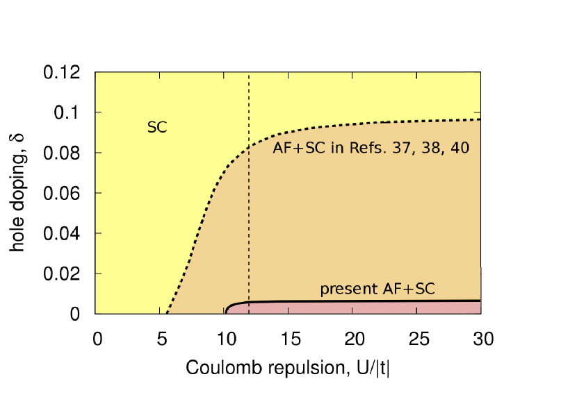
Figure 2: (Color online) Representative phase diagram for the $t$–$J$–$U$ model on the Coulomb repulsion – hole doping plane. The phases are labeled as follows: SC – superconducting phase, AF+SC – phase with coexisting superconducting and antiferromagnetic orders. The pure stable AF phase is found only for $\delta=0$ and for $U>10.6|t|$. The value $U/|t|=12$ marked by the dashed vertical line is taken in the subsequent analysis. The solid line is a our result. The dashed line is the result of previous studies (Refs. Yuan et al., 2005; Heiselberg, 2009; Liu et al., 2012).

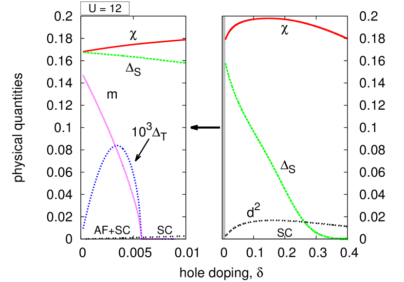
Figure 3: (Color online) Selected bare physical quantities $\chi_{AB}$, $\Delta_{S}$, $\Delta_{T}$, $m_{AF}$, and $d^{2}$, all as a function of doping $\delta$ and for $U/|t|=12$. In the coexistent AF+SC phase we have $\Delta_{S}\neq 0$, $\Delta_{T}\neq 0$, and $m_{AF}\neq 0$. Such phase is stable only in the vicinity of the half-filling, as detailed in the left panel where $\delta\in[0,\,0.01]$. On the right panel we present overall behavior in the wider range of the doping.).

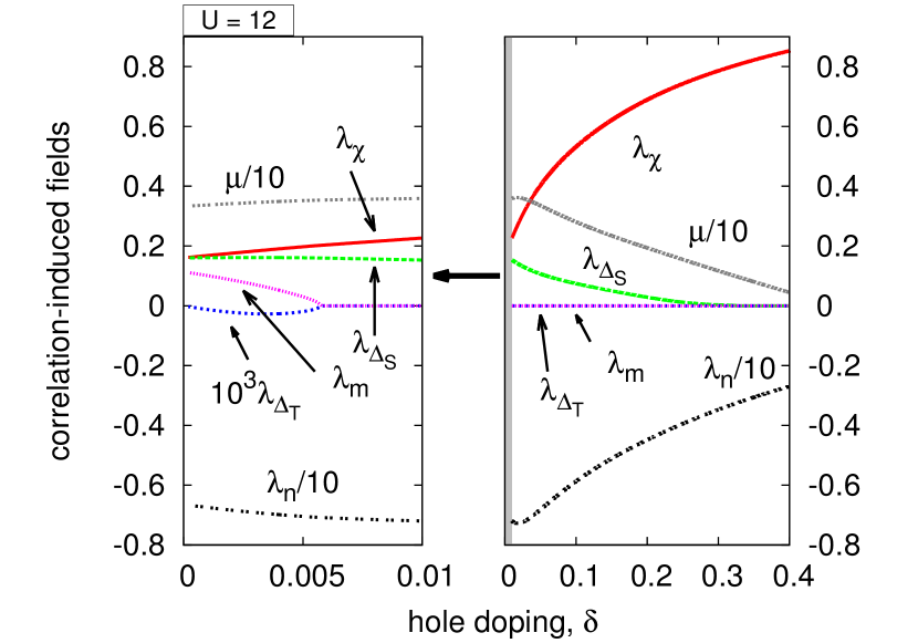
Figure 4: (Color online) Correlation-induced fields $\lambda{\chi_{AB}}$, $\lambda_{\Delta_{S}}$, $\lambda_{\Delta_{T}}$, $\lambda_{m}$, and the chemical potential $\mu$, all as a function of doping $\delta$ for $U/|t|=12$. The fields $\{\lambda\}$ have non-zero values only when the corresponding mean fields are also non-zero. Note that on the left panel $\mu\sim W/2\sim 4|t|$, corresponding to the almost-filled lower Hubbard subband.

The correlated spin-singlet gap parameter in real space is defined as

$$\tau_{ij}\Delta^{c}_{S} = \frac{1}{4}\left(\left\langle\hat{c}_{i\in A\,\downarrow}\hat{c}_{j\in B\uparrow}\right\rangle-\left\langle\hat{c}_{i\in A\uparrow}\hat{c}_{j\in B\,\downarrow}\right\rangle+\mbox{H.c.}\right),$$ (16)

where the average is calculated using the Gutzwiller wave function $\left|\Psi\right\rangle$, instead of $\left|\Psi_{0}\right\rangle$. Approximately (within GA), the correlated (physical) SC order parameters can be expressed asYuan et al. (2005); Heiselberg (2009)

$$\Delta^{c}_{S} = g_{\Delta}\Delta_{S},\hskip 12.0pt\mbox{and}\hskip 12.0pt\Delta^{c}_{T}=g_{\Delta}\Delta_{T},$$ (17)

where

$$g_{\Delta} = \frac{n-2d^{2}}{2(n-2rw)}\left[\left(\sqrt{\frac{(1-w)(1-n+d^{2})}{1-r}}+\sqrt{\frac{wd^{2}}{r}}\right)^{2}\right.+$$ (18)

$$+\left.\left(\sqrt{\frac{(1-r)(1-n+d^{2})}{1-w}}+\sqrt{\frac{rd^{2}}{w}}\right)^{2}\right].$$

The AF order parameter, and the renormalized hopping parameter are defined in a similar manner, specifically

$$m^{c}_{AF} = g_{m}\,m_{AF},$$ (19)

$$\chi^{c}_{AB} = g_{t}\,\chi_{AB},$$ (20)

where $g_{t}$ is presented in Eq. (4a) and

$$g_{m} = \frac{n-2d^{2}}{n-2wr}.$$ (21)

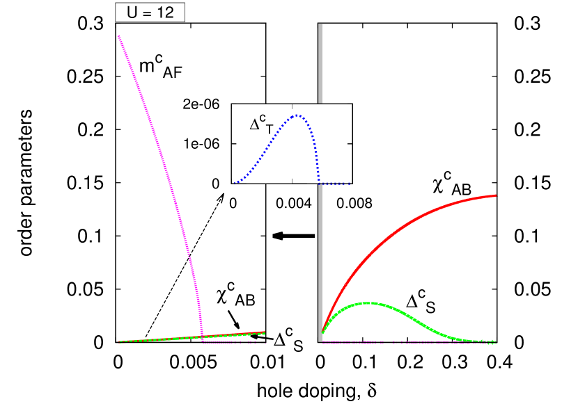
Figure 5: (Color online) Order parameters of SC and AF states in the correlated state versus doping $\delta$ and for $U/|t|=12$. AF disappears for $\delta\approx 6\cdot 10^{-3}$. In the limit $\delta=0$ the state transforms into an AF insulator. For $\delta\gtrsim 0.1$, the hopping amplitude $\chi^{c}_{AB}$ increases substantially. Inset: dependence of $\Delta^{c}_{T}$ in the vicinity of the half-filling. Note, that the value of $\Delta^{c}_{T}$ is about $10^{4}$ times smaller than the value of $\Delta^{c}_{S}$.

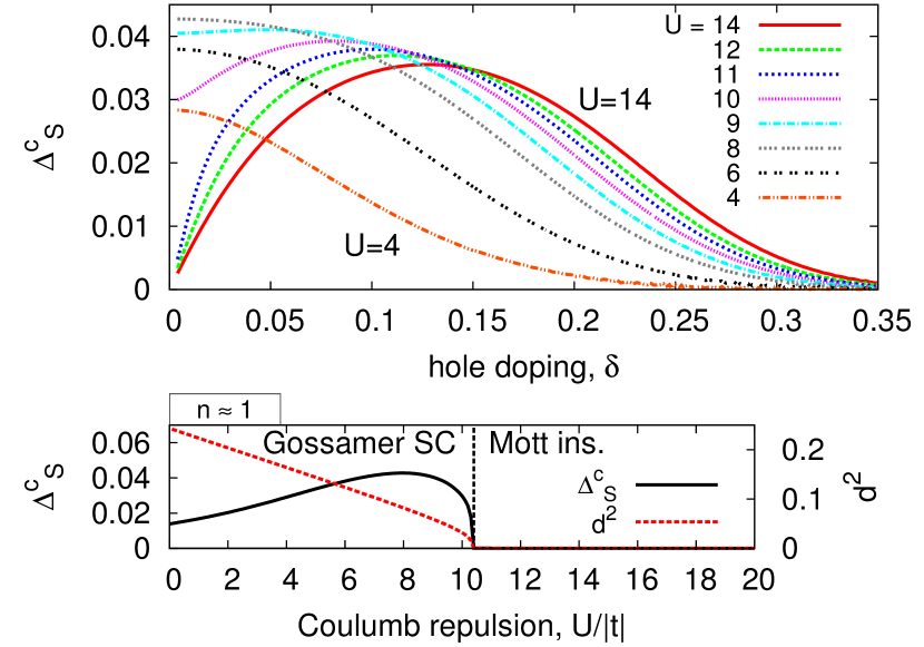
Figure 6: (Color online) Profile of the correlated singlet gap $\Delta^{c}_{S}$ for selected values of $U/|t|$ versus hole-doping (top). The limiting values of $\Delta^{c}_{S}$ and $d^{2}$ for $n\approx 1$ are presented in the bottom panel.

The magnitude of $\Delta_{T}^{c}$ is about $10^{4}$ times smaller than the magnitude of $\Delta_{S}^{c}$, so most probably, it may not be observable. For $\delta\gtrsim 1/3$ the order parameter $\Delta_{S}^{c}$ decrease exponentially. Note a spectacular increase of the hopping probability $\chi^{c}_{AB}$ with increased doping in Fig. 5, leading to an effective Fermi liquid state for $\delta\gtrsim 1/3$.

The non-zero correlated gap at $n=1$ for low-$U$ values provides an evidence for a gossamer superconductivity. The concept of gossamer superconductivity was introduced by LaughlinLaughlin (2006) and it describes the situation when the pure SC phase is stable at the half-filling. For $U/|t|\approx 10.6$ and $n=1$, where AF+SC phase sets in, the correlated gap $\Delta^{c}_{S}$ vanishes. Details of the transition are presented in Fig. 6, cf. the bottom panel. The critical $U/|t|$ value for the disappearance of $\Delta_{S}$ is marked by the dotted vertical line.

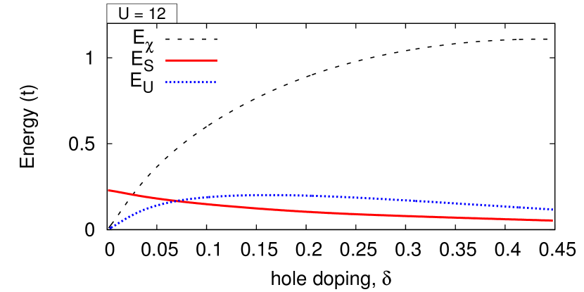
Figure 7: (Color online) The optimized component energies composing the total energy (Eq. (9), which represent $T\rightarrow 0$ limit of Eq. (13)). For discussion see main text.

In the sake of completeness, we have drawn for $U=12|t|$ in Fig. 7 the components of the total energy (Eq. (13)), to show that in the underdoped regime the effective hopping energy $E_{\chi}\equiv 8g_{t}|t|\chi_{AB}$, the total exchange contribution $E_{S}\equiv g_{s}J\left(m_{AF}^{2}/2+3\chi^{2}_{AB}+3\Delta^{2}_{S}-\Delta^{2}_{T}\right)$, and the Coulomb energy $E_{U}=Ud^{2}$, are all of comparable magnitude. This is the regime of strong correlations.

The overall behavior of the obtained characteristics can be summarized as follows. First, the coexistent AF+SC phase appears only for the doping $\delta<0.006$ and transforms into the pure Mott insulating state (AF) only at the half filling $\delta=0$ and large $U$. The spin-triplet gap component is practically negligible in the AF+SC phase. Introducing the molecular fields $\lambda_{\chi}$, $\lambda_{\Delta_{S}}$, and $\lambda_{m}$ (where non-zero), and $\lambda_{n}$ change the phase diagram in a significant manner which means, that the influence of the consistency constraints on the single-particle states is important. The spin-singlet $d$-wave superconductivity vanishes exponentially for large $\delta$. The optimal doping appears in the interval $\delta\sim 0.1$ – $0.15$ and is weakly dependent on $U$ for $U\gtrsim 12|t|$.

V Conclusions and comments

Using the statistically-consistent Gutzwiller approximation (SGA), we have analyzed in detail the effective Hamiltonian considered previously in Refs. Yuan et al., 2005; Heiselberg, 2009; Liu et al., 2012. However, in contrast to those papers, we have considered a more complete structure of the SC gap (the components $\Delta_{S}$ and $\Delta_{T}$). Also, a significantly narrower region of the coexistence of AF and SC is obtained. Furthermore, the critical value of $U$ for AF+SC appearance is higher, and for $J/|t|=1/3$ the value is about $10.6|t|$. We have checked that the bare amplitude $\Delta_{T}$ is about $10^{3}$ times smaller than that of $\Delta_{S}$ (similarly, the order parameters ratio $\Delta_{T}^{c}/\Delta_{S}^{c}\approx 10^{-4}$). We have checked that when the $\Delta_{T}$ is omitted, the results do not change in any significant manner. Therefore, the spin-triplet component of the superconducting order is most probably not detectable experimentally.

In previous studies (cf. Refs. Yuan et al., 2005; Heiselberg, 2009; Liu et al., 2012) a much wider coexistence region was reported. In the present paper, we correct those predictions (cf. Fig. 2). Namely, we show, that the previous results were an effect of the non-statistically consistent RMFT approach used. Illustratively, in Ref. Yuan et al., 2005, a minimization procedure is formulated by setting $\partial E_{\mbox{var}}/\partial m=0$, yielding Eq. (21) in Ref. Yuan et al., 2005 for $m$ which is different than that defining $m$ [cf. Eq. (16) in Ref. Yuan et al., 2005]. We claim that a more correct approach is provided by SGA, where the Lagrange multipliers are introduced for each operator for which the average appears in the effective mean-field Hamiltonian. In other words, without incorporating the multipliers, the free energy functional $\mathcal{F}$ is minimized in an over-extended Fock space containing, along with physical configurations, also those that lead to the statistical inconsistency. Using the constraints introduced by SGA, this space is limited to a subspace, in which such an inconsistency does not appear. Hence, the energy obtained in SGA can either be equal to or even higher than the energy obtained using non-consistent approaches. Obviously, this circumstance should not be used as an argument against SGA. Different formulations, where the model is solved in a self-consistent manner are also presented in Refs. Bünemann, 2005; Yang, 2009.

As said above, in the SGA method, an effective single-particle approach with conditions (14) is developed. In such an approach the question of a pseudogap is not addressed. This is because (i) the order parameter $\Delta_{S}$ is assumed as real (i.e., no phase fluctuation appears), and (ii) the collective spin degrees of freedom are not separated from single-particle fermionic correlations. In order to address that issue, one would have to generalize the approach to include, e.g., the spin sector of the excitations,Feng et al. (2012) even in the absence of AF order. As the antiferromagnetism is built into the SGA approach automatically, work on extension of this approach to include magnetic fluctuations in the paramagnetic phase is in progress.

One should note that the definition of the Mott (or Mott-Hubbard) insulator here complements that for the Hubbard model within the standard Gutzwiller approximation (GA) which represents the infinite-dimension variant of the approach.Kubo and Uchinami (1975) Namely, with an assumption that $J\neq 0$ we have a gradual evolution of the antiferromagnetic order parameter $m_{AF}\rightarrow 1$ with the increasing $U$, i.e., the system evolves from the Slater to the Mott antiferromagnet. This is what is also obtained in the saddle-point approximation within the slave-boson approach,Korbel et al. (2003) which differs from the standard GA by incorporating constraints, some of them of similar character as those introduced here in SGA. In this respect both SGA and the saddle-point approximation to slave-boson approach go beyond GA, albeit not in an explicitly systematic formal manner.

Appendix A Definitions of the mean-fields and evaluation of $\left\langle\mathcal{\mathcal{\hat{H}}}_{\mathit{eff}}\right\rangle_{0}\equiv W$

In the main text, the uniform bond order parameter for $i$ and $j$ sites indicating the nearest neighboring sites is defined as $\langle\hat{c}^{\dagger}_{i\sigma}\hat{c}_{j\sigma}\rangle_{0}\equiv\chi_{AB}$. It was assumed that $\langle\hat{c}^{\dagger}_{i\sigma}\hat{c}_{j\sigma}\rangle_{0}$ is real. Let us consider in this appendix a more general form. Since the sublattice $A$ contains the sites where the majority spin is $\uparrow$ and the sublattice $B$ the sites where majority spin is $\downarrow$, the general form can be written as

$$\langle\hat{c}_{i\in A\uparrow}^{\dagger}\hat{c}_{j\in B\uparrow}\rangle_{0}=\langle\hat{c}_{j\in B\downarrow}^{\dagger}\hat{c}_{i\in A\downarrow}\rangle_{0}=\langle\hat{c}_{i\in A\downarrow}^{\dagger}\hat{c}_{j\in B\downarrow}\rangle_{0}^{*}=\chi_{o-c},$$ (22)

$$\langle\hat{c}_{i\in A\downarrow}^{\dagger}\hat{c}_{j\in B\downarrow}\rangle_{0}=\langle\hat{c}_{j\in B\uparrow}^{\dagger}\hat{c}_{i\in A\uparrow}\rangle_{0}=\langle\hat{c}_{i\in A\uparrow}^{\dagger}\hat{c}_{j\in B\uparrow}\rangle_{0}^{*}=\chi_{c-o},$$ (23)

for $i$ and $j$ being the nearest neighbors, where $\chi_{o-c}$ is an average of the operator describing the hopping of an electron from a site, where the average spin is opposite to the spin of the electron, to the site, where the average spin is congruent to the spin of the electron. $\chi_{o-c}$ describes the opposite situation. This results in the general expression that

$$\chi_{ij\sigma}\equiv\langle\hat{c}^{\dagger}_{i\sigma}\hat{c}_{j\sigma}\rangle_{0}=\chi_{AB}+i\sigma e^{i{\bf Q}\cdot{\bf R}_{i}}\delta\chi_{AB},$$ (24)

where $\chi_{AB}\equiv\frac{1}{2}\left(\chi_{o-c}+\chi_{c-o}\right)$ and $\delta\chi_{AB}\equiv\frac{1}{2i}\left(\chi_{o-c}-\chi_{c-o}\right)$.

The electron-pairing order parameter for the nearest neighbors is defined as

$$\Delta_{ij\downarrow}\equiv\left\langle\hat{c}_{j\,\downarrow}\hat{c}_{i\uparrow}\right\rangle_{0}\equiv\left\{\begin{array}[]{ll}\tau_{ij}\tilde{\Delta}_{A},&\text{for $i\in A$},\\ \tau_{ij}\tilde{\Delta}_{B},&\text{for $i\in B$},\end{array}\right.$$ (25)

where $\tau_{ij}\equiv 1$ for $j=i\pm\hat{x}$ and ${\tau_{ij}\equiv-1}$ for $j=i\pm\hat{y}$ ($\Delta_{ij\uparrow}$ is defined in simillar manner). For the staggered magnetic moment $m_{AF}=0$ one can assume that $\tilde{\Delta}_{A}=\tilde{\Delta}_{B}$. However, when $m_{AF}\neq 0$, the order parameter $\tilde{\Delta}_{A}$ is a product of two operators, both of which annihilate electrons whose spin is congruent to the average spin of individual sites. On the contrary, $\tilde{\Delta}_{B}$ is a product of two operators that annihilate electrons whose spin is opposite to the average spin of individual sites. Hence, it may be that $\tilde{\Delta}_{A}\neq\tilde{\Delta}_{B}$. Also, similar as with the hopping amplitude, $\tilde{\Delta}_{A}$ and $\tilde{\Delta}_{B}$ might be complex numbers. Let us denote $\tilde{\Delta}_{A}\equiv(\Delta_{A},\ \delta\Delta_{A})$ and $\tilde{\Delta}_{B}\equiv(\Delta_{B},\ \delta\Delta_{B})$, where the parameters in brackets are the real and imaginary parts of the corresponding gaps, respectively.

The only nontrivial part of $\left\langle\mathcal{\mathcal{\hat{H}}}_{\mathit{eff}}\right\rangle_{0}$ [cf. Eq. (3)] can be evaluated in the form

$$4\langle{\bf\hat{S}}_{i}\cdot{\bf\hat{S}}_{j}\rangle_{0}\approx-\left(\left\langle\hat{c}_{i\downarrow}^{\dagger}\hat{c}_{i\downarrow}\right\rangle_{0}-\left\langle\hat{c}_{i\uparrow}^{\dagger}\hat{c}_{i\uparrow}\right\rangle_{0}\right)^{2}\\ -\left(\left\langle\hat{c}_{i\downarrow}^{\dagger}\hat{c}_{j\downarrow}\right\rangle_{0}+2\left\langle\hat{c}_{i\uparrow}^{\dagger}\hat{c}_{j\uparrow}\right\rangle_{0}\right)\left\langle\hat{c}_{j\downarrow}^{\dagger}\hat{c}_{i\downarrow}\right\rangle_{0}\\ -\left(2\left\langle\hat{c}_{i\downarrow}^{\dagger}\hat{c}_{j\downarrow}\right\rangle_{0}+\left\langle\hat{c}_{i\uparrow}^{\dagger}\hat{c}_{j\uparrow}\right\rangle_{0}\right)\left\langle\hat{c}_{j\uparrow}^{\dagger}\hat{c}_{i\uparrow}\right\rangle_{0}\\ -\left(-\left\langle\hat{c}_{i\uparrow}\hat{c}_{j\downarrow}\right\rangle_{0}+2\left\langle\hat{c}_{i\downarrow}\hat{c}_{j\uparrow}\right\rangle_{0}\right)\left\langle\hat{c}_{i\uparrow}^{\dagger}\hat{c}^{\dagger}_{j\downarrow}\right\rangle_{0}\\ -\left(2\left\langle\hat{c}_{i\uparrow}\hat{c}_{j\downarrow}\right\rangle_{0}-\left\langle\hat{c}_{i\downarrow}\hat{c}_{j\uparrow}\right\rangle_{0}\right)\left\langle\hat{c}_{i\downarrow}^{\dagger}\hat{c}^{\dagger}_{j\uparrow}\right\rangle_{0},$$ (26)

where we have applied the Wick’s theorem and we have assumed that $\left\langle\hat{c}_{i\uparrow}^{\dagger}\hat{c}_{i\downarrow}\right\rangle_{0}\equiv 0$, $\left\langle\hat{c}_{i\uparrow}\hat{c}_{i\downarrow}\right\rangle_{0}\equiv 0$, and $\left\langle\hat{c}_{i\downarrow}\hat{c}_{j\downarrow}\right\rangle_{0}=\left\langle\hat{c}_{i\uparrow}\hat{c}_{j\uparrow}\right\rangle_{0}\equiv 0$. Using the notation introduced above and Eq. (5), we have

$$4\langle{\bf\hat{S}}_{i}\cdot{\bf\hat{S}}_{j}\rangle_{0}=-m_{AF}^{2}-6\chi_{AB}^{2}+2(\delta\chi_{AB})^{2}\\ -|\tilde{\Delta}_{A}|^{2}-|\tilde{\Delta}_{B}|^{2}-4\tilde{\Delta}_{A}\tilde{\Delta}_{B}.$$ (27)

Since the above expression is invariant with respect to the same rotations of both vectors $\tilde{\Delta}_{A}$ and $\tilde{\Delta}_{B}$, one component of the vectors can be assumed to be eliminated. With the choice $\delta\Delta_{A}=0$, we have

$$\Delta_{ij\sigma}\equiv\langle\hat{c}_{i\sigma}\hat{c}_{j\bar{\sigma}}\rangle_{0}\equiv-\tau_{ij}\left(\sigma\Delta_{S}+e^{i{\bf Q}\cdot{\bf r}_{i}}\Delta_{T}\right)\\ -\tau_{ij}\frac{1}{2}i\left(\sigma-e^{i{\bf Q}\cdot{\bf r}_{i}}\right)\delta\Delta_{B},$$ (28)

where $\Delta_{S}\equiv\Delta_{A}+\Delta_{B}$ and $\Delta_{T}\equiv\Delta_{A}-\Delta_{B}$.

Therefore, the $\left\langle\mathcal{\mathcal{\hat{H}}}_{\mathit{eff}}\right\rangle_{0}\equiv W$ can be presented in the full form

$$\frac{W}{\Lambda}=8g_{t}t\chi_{AB}+Ud^{2}-g_{s}J\left(\frac{1}{2}m_{AF}^{2}+3\chi_{AB}^{2}-(\delta\chi_{AB})^{2}\right.\\ \left.+3\Delta_{S}^{2}-\Delta_{T}^{2}+\frac{1}{2}(\delta\Delta_{B})^{2}\right).$$ (29)

Introduction of $\delta\chi_{AB}$ and $\delta\Delta_{B}$ affects the form of selecting the correlated fields $\lambda^{\chi}_{ij\sigma}$ and $\lambda^{\Delta}_{ij\sigma}$, and the final set of necessary conditions for a local minimum of the free energy (cf. Eqs. (11b), (11c) and (14)). However, it was found that the state with the lowest energy (for the considered model) has always been that with $\delta\chi_{AB}\equiv 0$ and $\delta\Delta_{B}\equiv 0$. Hence, it is acceptable to neglect both terms and clame that $\Delta_{ij\sigma}$ and $\chi_{ij\sigma}$ are both real. For simplicity and clarity it is how the averages are presented in the main text. Finally, Eq. (29) is reduced to Eq. (9).

Appendix B Determination of the grand potential functional (Eq. (13))

To diagonalize $\hat{K}$ [Eq. (10)], we first perform the space Fourier transform. The result can be rewritten in the following $4\times 4$ matrix form

$$\hat{K}=W+\sum_{\bf k}{}^{{}^{\prime}}\hat{\Psi}_{\bf k}^{\dagger}\mathbbm{\tilde{M}}_{\bf k}\hat{\Psi}_{\bf k}+\frac{1}{2}\Lambda\left(\lambda_{n}(n-1)+\lambda_{m}m_{AF}\right)\\ -\Lambda\mu+8\Lambda\lambda_{\chi}\chi_{AB}+8\Lambda\left(\lambda_{\Delta_{S}}\Delta_{S}+\lambda_{\Delta_{T}}\Delta_{T}\right),$$ (30)

where $\hat{\Psi}^{\dagger}_{\bf k}=\begin{pmatrix}\hat{c}^{\dagger}_{{\bf k}\uparrow},&\hat{c}_{-{\bf k}\downarrow},&\hat{c}^{\dagger}_{{\bf k}+{\bf Q}\uparrow},&\hat{c}_{-{\bf k}+{\bf Q}\downarrow}\end{pmatrix}$, the sum is evaluated over the reduced (magnetic) Brillouin zone (${|k_{x}|+|k_{y}|\leqslant\pi}$), and

$$\mathbbm{\tilde{M}}_{\bf k}=\begin{pmatrix}-\lambda_{\chi}\epsilon_{{\bf k}}-\frac{1}{2}\lambda_{n}-\mu&-\lambda_{\Delta_{S}}\eta_{{\bf k}}&-\frac{1}{2}\lambda_{m}&\lambda_{\Delta_{T}}\eta_{{\bf k}}\\ -\lambda_{\Delta_{S}}\eta_{{\bf k}}&\lambda_{\chi}\epsilon_{{\bf k}}+\frac{1}{2}\lambda_{n}+\mu&-\lambda_{\Delta_{T}}\eta_{{\bf k}}&-\frac{1}{2}\lambda_{m}\\ -\frac{1}{2}\lambda_{m}&-\lambda_{\Delta_{T}}\eta_{{\bf k}}&\lambda_{\chi}\epsilon_{{\bf k}}-\frac{1}{2}\lambda_{n}-\mu&\lambda_{\Delta_{S}}\eta_{{\bf k}}\\ \lambda_{\Delta_{T}}\eta_{{\bf k}}&-\frac{1}{2}\lambda_{m}&\lambda_{\Delta_{S}}\eta_{{\bf k}}&-\lambda_{\chi}\epsilon_{{\bf k}}+\frac{1}{2}\lambda_{n}+\mu\end{pmatrix},$$ (31)

where for the square lattice

$$\epsilon_{{\bf k}} \equiv 2\left(\cos k_{x}+\cos k_{y}\right),$$ (32a)

$$\eta_{{\bf k}} \equiv 2\left(\cos k_{x}-\cos k_{y}\right).$$ (32b)

Diagonalization of $\mathbbm{\tilde{M}}_{\bf k}$ yields four branches of eigenvalues with their explicit form

$$E_{l{\bf k}}\equiv E_{\pm\,\pm\,{\bf k}} = \pm\frac{1}{2}\sqrt{K_{1{\bf k}}\pm 2\sqrt{K_{2{\bf k}}}},$$ (33)

where $l=1,\ldots,4$, and

$$K_{1{\bf k}} \equiv 4\epsilon_{{\bf k}}^{2}\lambda_{\chi}^{2}+\left(\lambda_{n}+2\mu\right)^{2}$$

$$+4\eta_{{\bf k}}^{2}\left(\lambda_{\Delta_{S}}^{2}+\lambda_{\Delta_{T}}^{2}\right)+\lambda_{m}^{2},$$ (34a)

$$K_{2{\bf k}} \equiv \left(4\eta_{{\bf k}}^{2}\lambda_{\Delta_{S}}\lambda_{\Delta_{T}}+\lambda_{m}\left(\lambda_{n}+2\mu\right)\right)^{2}$$

$$+\ 4\epsilon_{{\bf k}}^{2}\lambda_{\chi}^{2}\left(4\eta_{{\bf k}}^{2}\lambda_{\Delta_{T}}^{2}+\left(\lambda_{n}+2\mu\right)^{2}\right).$$ (34b)

The energies $\{E_{l{\bf k}}\}_{l=1,\ldots,4}$ represent quasiparticle bands after all parameters (mean-fields parameters, the Lagrange multipliers, and $d$) are determined variationally.

The generalized grand potential functional at temperature $T>0$ as given by

$$\mathcal{F}=-\frac{1}{\beta}\ln{\mathcal{Z}},\hskip 6.0pt\mbox{with}\hskip 6.0pt\mathcal{Z}=\mathrm{Tr}\left(e^{-\beta\hat{K}}\right),$$ (35)

and $\beta\equiv 1/k_{B}T$, thus

$$\mathcal{F}/\Lambda=8g_{t}t\chi_{AB}-g_{s}J\left(\frac{1}{2}m_{AF}^{2}+3\chi_{AB}^{2}+3\Delta_{S}^{2}-\Delta_{T}^{2}\right)\\ +\frac{1}{2}\lambda_{n}(n-1)+\frac{1}{2}\lambda_{m}m_{AF}+8\left(\lambda_{\chi}\chi_{AB}+\lambda_{\Delta_{S}}\Delta_{S}+\lambda_{\Delta_{T}}\Delta_{T}\right)\\ -\frac{1}{\Lambda\beta}\sum_{l,{\bf k}}\ln(1+e^{-\beta E_{l{\bf k}}})+Ud^{2}-\mu.$$ (36)

Appendix C Explicit form of the conditions for the minimum of $\mathcal{F}$

The necessary conditions for the minimum of $\mathcal{F}$, subject to all constraints (introduced in Eq. (10)) are

$$\frac{\partial\mathcal{F}}{\partial\vec{A}}=0,\hskip 6.0pt\hskip 6.0pt\frac{\partial\mathcal{F}}{\partial\vec{\lambda}}=0,\hskip 6.0pt\mbox{and}\hskip 6.0pt\frac{\partial\mathcal{F}}{\partial d}=0,$$ (37)

where the five mean-field parameters are labeled collectively as $\vec{A}$, the five Lagrange multipliers as $\vec{\lambda}$, and $d^{2}$ is double occupancy probability. In explicit form $\partial\mathcal{F}/\partial\vec{A}=0$ stands for

$$\lambda_{\chi}=-g_{t}t+\frac{3}{4}g_{s}J\chi_{AB},$$ (38a)

$$\lambda_{\Delta_{S}}=\frac{3}{4}g_{s}J\Delta_{S},$$ (38b)

$$\lambda_{\Delta_{T}}=-\frac{1}{4}g_{s}J\Delta_{T},$$ (38c)

$$\lambda_{n}=-16t\chi_{AB}\frac{\partial g_{t}}{\partial n}$$

$$\hskip 12.0pt-2J\left(-\frac{1}{2}m_{AF}^{2}-3\chi_{AB}^{2}-3\Delta_{S}^{2}+\Delta_{T}^{2}\right)\frac{\partial g_{s}}{\partial n},$$ (38d)

$$\lambda_{m}=2g_{s}Jm_{AF}-16t\chi_{AB}\frac{\partial g_{t}}{\partial m_{AF}}$$

$$\hskip 12.0pt-2J\left(-\frac{1}{2}m_{AF}^{2}-3\chi_{AB}^{2}-3\Delta_{S}^{2}+\Delta_{T}^{2}\right)\frac{\partial g_{s}}{\partial m_{AF}},$$ (38e)

$\partial\mathcal{F}/\partial\vec{\lambda}=0$ can be evaluated as

$$\frac{1}{\Lambda}\sum_{{\bf k},l}f(E_{l{\bf k}})\,\partial_{\lambda_{\chi}}{E_{l{\bf k}}}+8\chi_{AB}=0,$$ (39a)

$$\frac{1}{\Lambda}\sum_{{\bf k},l}f(E_{l{\bf k}})\,\partial_{\lambda_{\Delta_{S}}}{E_{l{\bf k}}}+8\Delta_{S}=0,$$ (39b)

$$\frac{1}{\Lambda}\sum_{{\bf k},l}f(E_{l{\bf k}})\,\partial_{\lambda_{\Delta_{T}}}{E_{l{\bf k}}}+8\Delta_{T}=0,$$ (39c)

$$\frac{1}{\Lambda}\sum_{{\bf k},l}f(E_{l{\bf k}})\,\partial_{\lambda_{n}}{E_{l{\bf k}}}-\frac{1}{2}(1-n)=0,$$ (39d)

$$\frac{1}{\Lambda}\sum_{{\bf k},l}f(E_{l{\bf k}})\,\partial_{\lambda_{m}}{E_{l{\bf k}}}+\frac{1}{2}m_{AF}=0,$$ (39e)

and $\partial\mathcal{F}/\partial d=0$ denotes

$$2Ud+8t\chi_{AB}\frac{\partial g_{t}}{\partial d}$$

$$\hskip 12.0pt+J\left(-\frac{1}{2}m_{AF}^{2}-3\chi_{AB}^{2}-3\Delta_{S}^{2}+\Delta_{T}^{2}\right)\frac{\partial g_{s}}{\partial d}=0,$$ (40a)

where $f(E_{l{\bf k}})\equiv 1/\left(1+e^{\beta E_{l{\bf k}}}\right)$. Eqs. (38a)–(38e) can be used to eliminate the parameters $\{\lambda\}$ from the numerical solution procedure, reducing the number of algebraic equations to six. Consequently, we are left with Eqs. (39a)–(39e) (the conditions ${\partial\mathcal{F}/\partial\vec{\lambda}=0}$) and Eq. (40a) ($\partial\mathcal{F}/\partial d=0$).

Table 1: Values of the parameters obtained for the SC phase ($U/|t|=5$ and $\delta=0.3$) (example 1), for SC phase ($U/|t|=12$ and $\delta=0.03$) (example 2), and for the AF+SC phase ($U/|t|=12$ and $\delta=0.001$). The calculations were made for the lattice with $\Lambda=1024\times 1024$ sites. The numerical accuracy is at the last digit specified.

Variable	SC (1)	SC (2)	AF+SC
$\chi_{AB}$	$0.1907587$	$0.1887189$	$0.1693210$
$\Delta_{S}$	$0.00027$	$0.138176$	$0.166906$
$\Delta_{T}$	$0$	$0$	$3.92\cdot 10^{-5}$
$\mu$	$0.5664$	$3.5570$	$3.37154$
$m_{AF}$	$0$	$0$	$0.13194$
$d^{2}$	$5.22266\cdot 10^{-2}$	$8.16196\cdot 10^{-3}$	$2.2406\cdot 10^{-4}$
$\lambda_{\chi}$	$0.9661403$	$0.327769$	$0.168074$
$\lambda_{\Delta_{S}}$	$0$	$0.1258974$	$0.160777$
$\lambda_{\Delta_{T}}$	$0$	$0$	$1.2595\cdot 10^{-5}$
$\lambda_{n}$	$-2.526087$	$-7.176836$	$-6.744724$
$\lambda_{m}$	$0$	$0$	$0.100911$
$W$	$-1.150925$	$-0.33669191$	$-0.233031$
$g_{t}$	$0.884438$	$0.1558210$	$4.97139\cdot 10^{-3}$
$g_{s}$	$1.713202$	$3.644549$	$3.85310$
$g_{\Delta}$	$0.884438$	$0.1558210$	$4.99912\cdot 10^{-3}$
$g_{m}$	$1.3088937$	$1.9090702$	$1.96293$
$\chi^{c}_{AB}$	$0.1687143$	$2.94064\cdot 10^{-2}$	$8.41761\cdot 10^{-4}$
$\Delta^{c}_{S}$	$0.00024$	$2.15306\cdot 10^{-2}$	$8.343884\cdot 10^{-4}$
$\Delta^{c}_{T}$	$0$	$0$	$1.960\cdot 10^{-8}$
$m^{c}_{AF}$	$0$	$0$	$0.25900$

Appendix D An alternative procedure of introducing the constraints via Lagrange multipliers

In the main text we work with the mean-field grand Hamiltonian $\hat{K}$, defined as $\hat{K}\equiv W-\sum_{\iota}\left(\lambda_{\iota}\left(\hat{O}_{\iota}-O_{\iota}\right)+\mbox{H.c.}\right)-\mu\hat{N}$, where $W\equiv\left\langle\mathcal{\hat{H}}_{\mathit{eff}}\right\rangle_{0}$ (cf. Eqs. (3) and  (9)), and $\{\hat{O}_{\iota}\}$ are those operators, whose averages are used to construct $W$. Lagrange multipliers $\lambda_{\iota}$ are introduced to ensure self-consistency of the solution, i.e., $O_{\iota}\equiv\left\langle\hat{O}_{\iota}\right\rangle_{0}$ (cf. Eq. (10)).

Next, in order to find optimal (equilibrium) values of mean fields, the grand potential functional $\mathcal{F}=-{\beta}^{-1}\ln{\mathcal{Z}}$, where $\mathcal{Z}=\mathrm{Tr}\left(e^{-\beta\hat{K}}\right)$ (cf. Eq. (12)) is subsequently minimized with respect to mean-fields subject to constraints included in $\hat{K}$.

An alternative procedure to the one sketched above is to add the self-consistency preserving constraints directly to $\mathcal{\hat{H}}_{\mathit{eff}}^{\mathit{MF}}$, i.e., to the mean-field approximated $\mathcal{\hat{H}}_{\mathit{eff}}$. In this formulation, we have again a separate Lagrange multiplier $\lambda_{\iota}^{\prime}$ for each mean-field average $O_{\iota}^{\prime}\equiv\left\langle\hat{O}_{\iota}^{\prime}\right\rangle_{0}$ present in $\mathcal{\hat{H}}_{\mathit{eff}}^{\mathit{MF}}$. In effect, we construct the effective mean-field Hamiltonian of the form $\mathcal{\hat{H}}_{\lambda}\equiv\mathcal{\hat{H}}_{\textit{eff}}^{\textit{MF}}-\sum_{\iota}\left(\lambda_{\iota}^{\prime}\left(\hat{O}_{\iota}^{\prime}-O_{\iota}^{\prime}\right)+\mbox{H.c.}\right)$ and the corresponding mean-field grand Hamiltonian $\hat{K}^{\prime}\equiv\mathcal{\hat{H}}_{\lambda}-\mu\hat{N}$. As a next step, the functional $\mathcal{F^{\prime}}$ is constructed (exactly as discussed above). It should be noted, that minimization of $\mathcal{F^{\prime}}$ subject to constraints included in $\mathcal{\hat{H}}_{\lambda}$, leads to a set of equations different than Eqs. (38a)–(40a). However, those two procedures are equivalent, i.e., the optimal (equilibrium) values of the mean-fields, corresponding to the minimum of $\mathcal{F}$ and $\mathcal{F^{\prime}}$ (subject to the same constraints), coincide. A difference in the results may occur only for the values of the Lagrange multipliers, but this does not affect the equilibrium values of the calculated physical quantities. Hence, the two approaches are formally equivalent, which can be shown analytically and has also been verified numerically.

Those two approaches differ also with respect to numerical execution. Namely, within the first procedure, we can easily find the functional dependence of Lagrange multipliers $\vec{\lambda}_{\iota}$ on mean fields $O_{\iota}$ (as shown in Appendix C). As a result, the number of equations to be solved numerically is reduced by a factor of $2$. In the second approach discussed here, the corresponding equations for $\vec{\lambda}_{\iota}^{\prime}$ are much more complicated and it is not possible to solve them analytically. Therefore, one cannot reduce the effort and numerical cost of solving the model at the same time. So, even though the latter method appears more intuitively appealing, as being more similar to the standard mean-field approach, we have used the former method in the discussion in the main text.

Appendix E Supplementary informations

For the sake of completeness [cf. Table 1] we provide the representative values of the parameters calculated for the following phases: SC for ($U/|t|=5$, $\delta=0.1$, and $U/|t|=12$, $\delta=0.03$), and AF+SC ($U/|t|=12$, $\delta=0.001$). The energies in the columns should not be compared directly, as they correspond to different sets of microscopic parameters. Numerical accuracy is at the level of the last digit specified.

References

- Spałek and Oleś (1977) J. Spałek and A. Oleś, Physica B+C 86–88, 375 (1977).
- Chao et al. (1977) K. A. Chao, J. Spałek, and A. M. Oleś, J. Phys. C 10, L271 (1977).
- Spałek (2007) J. Spałek, Acta Phys. Polon. A 111, 409 (2007).
- Anderson (1988) P. W. Anderson, in Frontiers and borderlines in many-particle physics, edited by R. A. Broglia and J. R. Schrieffer (North-Holland, Amsterdam, 1988), pp. 1–40.
- Dagotto (1994) E. Dagotto, Rev. Mod. Phys. 66, 763 (1994).
- Sarker et al. (1994) S. K. Sarker, C. Jayaprakash, and H. R. Krishnamurthy, Phys. C. Supercond. 228, 309 (1994).
- Sarker and Lovorn (2010) S. K. Sarker and T. Lovorn, Phys. Rev. B 82, 014504 (2010).
- Johnson et al. (2001) P. Johnson, A. Fedorov, and T. Valla, J. Electron. Spectrosc. Relat. Phenom. 117, 153 (2001).
- Lee et al. (2006) P. A. Lee, N. Nagaosa, and X.-G. Wen, Rev. Mod. Phys. 78, 17 (2006).
- Imada et al. (1998) M. Imada, A. Fujimori, and Y. Tokura, Rev. Mod. Phys. 70, 1039 (1998).
- Damascelli et al. (2003) A. Damascelli, Z. Hussain, and Z.-X. Shen, Rev. Mod. Phys. 75, 473 (2003).
- Tanaka et al. (206) K. Tanaka, W. S. Lee, D. H. Lu, A. Fujimori, T. Fujii, Risdiana, I. Terasaki, D. J. Scalapino, T. P. Devereaux, Z. Hussain, et al., Science 314, 1910 (206).
- Scalapino (2012) D. J. Scalapino, Rev. Mod. Phys. 84, 1383 (2012).
- Zhang and Rice (1988) F. C. Zhang and T. M. Rice, Phys. Rev. B 37, 3759 (1988).
- Zaanen and Sawatzky (1990) J. Zaanen and G. Sawatzky, J. Solid State Chem. 88, 8 (1990).
- Daul et al. (2000) S. Daul, D. J. Scalapino, and S. R. White, Phys. Rev. Lett. 84, 4188 (2000).
- Basu et al. (2001) S. Basu, R. J. Gooding, and P. W. Leung, Phys. Rev. B 63, 100506 (2001).
- Zhang (2003) F. C. Zhang, Phys. Rev. Lett. 90, 207002 (2003).
- Xiang et al. (2009) T. Xiang, H. G. Luo, D. H. Lu, K. M. Shen, and Z. X. Shen, Phys. Rev. B 79, 014524 (2009).
- Yu et al. (2007) W. Yu, J. S. Higgins, P. Bach, and R. L. Greene, Phys. Rev. B 76, 020503 (2007).
- Armitage et al. (2010) N. P. Armitage, P. Fournier, and R. L. Greene, Rev. Mod. Phys. 82, 2421 (2010).
- Kimura et al. (1999) H. Kimura, K. Hirota, H. Matsushita, K. Yamada, Y. Endoh, S.-H. Lee, C. F. Majkrzak, R. Erwin, G. Shirane, M. Greven, et al., Phys. Rev. B 59, 6517 (1999).
- Lee et al. (1999) Y. S. Lee, R. J. Birgeneau, M. A. Kastner, Y. Endoh, S. Wakimoto, K. Yamada, R. W. Erwin, S.-H. Lee, and G. Shirane, Phys. Rev. B 60, 3643 (1999).
- Sidis et al. (2001) Y. Sidis, C. Ulrich, P. Bourges, C. Bernhard, C. Niedermayer, L. P. Regnault, N. H. Andersen, and B. Keimer, Phys. Rev. Lett. 86, 4100 (2001).
- Hodges et al. (2002) J. A. Hodges, Y. Sidis, P. Bourges, I. Mirebeau, M. Hennion, and X. Chaud, Phys. Rev. B 66, 020501 (2002).
- Kawamoto et al. (2008) T. Kawamoto, Y. Bando, T. Mori, T. Konoike, Y. Takahide, T. Terashima, S. Uji, K. Takimiya, and T. Otsubo, Phys. Rev. B 77, 224506 (2008).
- Mathur et al. (1998) N. D. Mathur, F. M. Grosche, S. R. Julian, I. R. Walker, D. M. Freye, R. K. W. Haselwimmer, and G. G. Lonzarich, Nature 394, 39 (1998).
- Ma et al. (2012) L. Ma, G. F. Ji, J. Dai, X. R. Lu, M. J. Eom, J. S. Kim, B. Normand, and W. Yu, Phys. Rev. Lett. 109, 197002 (2012).
- Li et al. (2012) Z. Li, R. Zhou, Y. Liu, D. L. Sun, J. Yang, C. T. Lin, and G.-q. Zheng, Phys. Rev. B 86, 180501 (2012).
- Marsik et al. (2010) P. Marsik, K. W. Kim, A. Dubroka, M. Rössle, V. K. Malik, L. Schulz, C. N. Wang, C. Niedermayer, A. J. Drew, M. Willis, et al., Phys. Rev. Lett. 105, 057001 (2010).
- Bernhard et al. (2012) C. Bernhard, C. N. Wang, L. Nuccio, L. Schulz, O. Zaharko, J. Larsen, C. Aristizabal, M. Willis, A. J. Drew, G. D. Varma, et al., Phys. Rev. B 86, 184509 (2012).
- Milovanović and Predin (2012) M. V. Milovanović and S. Predin, Phys. Rev. B 86, 195113 (2012).
- Gan et al. (2005a) J. Y. Gan, F. C. Zhang, and Z. B. Su, Phys. Rev. B 71, 014508 (2005a).
- Gan et al. (2005b) J. Y. Gan, Y. Chen, Z. B. Su, and F. C. Zhang, Phys. Rev. Lett. 94, 067005 (2005b).
- Bernevig et al. (2003) B. A. Bernevig, R. B. Laughlin, and D. I. Santiago, Phys. Rev. Lett. 91, 147003 (2003).
- Laughlin (2006) R. B. Laughlin, Philosophical Magazine 86, 1165 (2006).
- Van Harlingen (1995) D. J. Van Harlingen, Rev. Mod. Phys. 67, 515 (1995).
- Tsuei and Kirtley (2000) C. C. Tsuei and J. R. Kirtley, Rev. Mod. Phys. 72, 969 (2000).
- Yuan et al. (2005) F. Yuan, Q. Yuan, and C. S. Ting, Phys. Rev. B 71, 104505 (2005).
- Heiselberg (2009) H. Heiselberg, Phys. Rev. A 79, 063611 (2009).
- Voo (2011) K.-K. Voo, J. Phys.: Condens. Matter 23, 495602 (2011).
- Liu et al. (2012) F.-F. Liu, Y. Zhang, F. Yuan, and L.-H. Xia, Communications in Theoretical Physics 57, 727 (2012).
- Jędrak et al. (2010) J. Jędrak, J. Kaczmarczyk, and J. Spałek, arXiv:cond-mat/1008.0021 (2010), unpublished.
- Jędrak and Spałek (2010) J. Jędrak and J. Spałek, Phys. Rev. B 81, 073108 (2010).
- Jędrak (2011) J. Jędrak, Ph.D. thesis, Jagiellonian University, Kraków (2011), URL http://th-www.if.uj.edu.pl/ztms/download/phdTheses/Jakub_Jedr%ak_doktorat.pdf.
- Gutzwiller (1963) M. C. Gutzwiller, Phys. Rev. Lett. 10, 159 (1963).
- Gutzwiller (1965) M. C. Gutzwiller, Phys. Rev. 137, A1726 (1965).
- Ogawa et al. (1975) T. Ogawa, K. Kanda, and T. Matsubara, Prog. Theor. Phys. 53, 614 (1975).
- Zhang et al. (1988) F. C. Zhang, C. Gros, T. M. Rice, and H. Shiba, Supercond. Sci. Technol. 1, 36 (1988).
- Himeda and Ogata (1999) A. Himeda and M. Ogata, Phys. Rev. B 60, R9935 (1999).
- Tsonis et al. (2008) S. Tsonis, P. Kotetes, G. Varelogiannis, and P. B. Littlewood, J. Phys.: Condens. Matter 20, 434234 (2008).
- Aperis et al. (2010) A. Aperis, G. Varelogiannis, and P. B. Littlewood, Phys. Rev. Lett. 104, 216403 (2010).
- Bogoliubov (1958a) N. N. Bogoliubov, Soviet Phys. JETP 34, 41 (1958a).
- Bogoliubov (1958b) N. N. Bogoliubov, Zh. Exp. Teor. Fiz. 34, 58 (1958b).
- Bogolyubov et al. (1958) N. N. Bogolyubov, V. V. Tolmachev, and D. V. Shirkov, Fortsch.Phys. 6, 605 (1958).
- Slater (1951) J. C. Slater, Phys. Rev. 82, 538 (1951).
- Kaczmarczyk and Spałek (2011) J. Kaczmarczyk and J. Spałek, Phys. Rev. B 84, 125140 (2011).
- Kaczmarczyk (2011) J. Kaczmarczyk, Ph.D. thesis, Jagiellonian University, Kraków (2011), URL http://th-www.if.uj.edu.pl/ztms/download/phdTheses/Jan_Kaczma%rczyk_doktorat.pdf.
- Note (1) Note1, with increase of hole-doping the approximation of zero temperature described in the main text became weaker. For bigger (e.q. for bigger than ) it starts be insufficient. Taking bigger moves the limiting value of just a little. Thus, for limit of strong hole-doping other computational techniques have to be used (since the correlations are weak in such limit, it can be a basic RMFT methods as described in Ref. Yuan et al., 2005).
- Galassi et al. (2009) M. Galassi, J. Davies, J. Theiler, B. Gough, P. Jungman, G. abd Alken, M. Booth, and F. Rossi, GNU Scientific Library Reference Manual (2009), 3rd ed., Network Theory, Ltd., London.
- Bünemann (2005) J. Bünemann, J. Phys.: Condens. Matter 17, 3807 (2005).
- Yang (2009) K.-Y. Yang, New J. Phys. 11, 055053 (2009).
- Feng et al. (2012) S. Feng, H. Zhao, and Z. Huang, Phys. Rev. B 85, 054509 (2012).
- Kubo and Uchinami (1975) K. Kubo and M. Uchinami, Prog. Theor. Phys 54, 1289 (1975).
- Korbel et al. (2003) P. Korbel, W. Wójcik, A. Klejnberg, J. Spałek, M. Acquarone, and M. Lavagna, Eur. Phys. J. B 32, 315 (2003).