Uncertainty of Weak Measurement and Merit of Amplification

Abstract

Aharonov’s weak value, which is a physical quantity obtainable by weak measurement, admits amplification and hence is deemed to be useful for precision measurement. We examine the significance of the amplification based on the uncertainty of measurement, and show that the trade-offs among the three (systematic, statistical and nonlinear) components of the uncertainty inherent in the weak measurement will set an upper limit on the usable amplification. Apart from the Gaussian state models employed for demonstration, our argument is completely general; it is free from approximation and valid for arbitrary observables $A$ and couplings $g$.

Introduction.

The novel physical quantity in quantum mechanics called weak value, proposed by Aharonov and co-workers long ago Aharonov_1964 ; Aharonov_1988 , has gained a renewed interest in recent years. One of the reasons for this is that, unlike the standard physical value given by an eigenvalue of an observable $A$, the weak value may be considered meaningful even for a set of non-commutable observables, simultaneously. This inspired a new insight for understanding counter-intuitive phenomena, such as the three-box paradox Aharonov_1991 and Hardy’s paradox Yokota_2009 . The other, perhaps stronger, motive comes from the realization that the weak value can be amplified by adjusting the process of measurement, weak measurement. Specifically, by choosing properly the initial and the final state (pre and postselection) of the process, the weak value can be made arbitrarily large, and this may be utilized for precision measurement. In fact, it has been reported that a significant amplification is achieved to observe successfully the spin Hall effect of light Hosten_2008 . A similar amplification has also been shown to be available for detecting ultrasensitive beam deflection in a Sagnac interferometer Dixon_2009 .

In view of this, it is quite natural to ask whether there exists a limit on amplification, and if so why. This question was addressed recently in Wu_2011 , which extended the treatment of Josza_2007 to the full order of the coupling $g$ between the system and the measurement device, where the amplification is analyzed based on the average shift of the meter of the device. For the particular case of the observable $A$ fulfilling $A^{2}=\mathrm{Id}$ and the Gaussian device states, it has been shown that the amplification rate, as well as the signal-to-noise ratio, has an upper limit Koike_2011 ; Nakamura_2012 . No such limit arises if the device state can be tuned precisely according to the weak value and the coupling Susa_2012 .

This Letter presents a completely new approach to the analysis of the weak value amplification. Rather than focusing on the shift of the meter, we consider the uncertainty of the weak measurement and inquire when it is meaningful as measurement for given particular purposes. This should be more important, because during the amplification the obtained amplified shift may well drift away from the intended weak value, rendering the whole measurement meaningless. Our uncertainty is defined from a probabilistic estimation on the deviation of the measured value from the weak value itself, and is shown to be separable into systematic, statistical, and nonlinear components. For the purpose of probing the existence of a physical effect, as done in the experiments Hosten_2008 ; Dixon_2009 , the condition of significant weak measurement is presented by demanding that the uncertainty (with the probability assigned beforehand) be smaller than the weak value to be measured. In the case of the Gaussian state, this explains the appearance of the range of amplification in which the existence of the effect is affirmed with assurance greater than the probability. The case also confirms the anticipation Aharonov_2005 that the weak value may be observed with non-small $g$, i.e., by ‘non-weak’ measurement. Apart from the Gaussian state analysis, our treatment is completely general; it is valid for an arbitrary dimensional system with arbitrary observables $A$ for all range of couplings $g$, and no approximation is used throughout (detailed discussions with mathematical proofs shall be given in Supplemental Material).

Weak Value and Weak Measurement.

We begin by recalling the process of weak measurement for obtaining the weak value. Let $\mathcal{H},\,\mathcal{K}$ be the Hilbert spaces associated with the system and that of the measuring device, respectively. We wish to find the value of an observable $A$ of the system represented by a self-adjoint operator on $\mathcal{H}$. This is done through the measurement of observables $Q$, $P$ of the meter device, which are represented by self-adjoint operators on $\mathcal{K}$ satisfying the canonical commutation relation $[Q,P]=i\hbar$ (we put $\hbar=1$ hereafter for brevity). Our measurement is assumed to be of von Neumann type, in which the evolution of the composite system $\mathcal{H}\otimes\mathcal{K}$ is described by the unitary operator $e^{-igA\otimes P}$ with a coupling parameter $g\in[0,\infty)$.

Prior to the interaction, the measured system shall be prepared in some state $|\phi_{i}\rangle\in\mathcal{H}$. Along with this preselection, the measuring device is also prepared in a state $|\psi_{i}\rangle\in\mathcal{K}$. The state of the composite system evolves after the interaction into $e^{-igA\otimes P}|\phi_{i}\rangle|\psi_{i}\rangle$. We then choose a state $|\phi_{f}\rangle\in\mathcal{H}$ on which a projective measurement in $\mathcal{H}$ is performed. Those that result in $|\phi_{f}\rangle$ shall be kept, otherwise discarded. After this postselection, the composite state will be disentangled into $|\phi_{f}\rangle|\psi_{f}\rangle$, where $|\psi_{f}\rangle=\langle\phi_{f}|e^{-igA\otimes P}|\phi_{i}\rangle|\psi_{i}\rangle$.

We intend to extract information of the triplet $(A,|\phi_{i}\rangle,|\phi_{f}\rangle)$ from the above measurement, and to this end we choose an observable $X=Q$ or $P$ of the measuring device and examine its shift in the expectation value $E_{X}(\psi):=\langle\psi|X|\psi\rangle/\|\psi\|^{2}$ between the two selections: $\Delta^{w}_{X}(g):=E_{X}(\psi_{f})-E_{X}(\psi_{i})$. Imposing certain conditions on $|\phi_{i}\rangle$ and $|\psi_{i}\rangle$, both the functions $g\mapsto\Delta^{w}_{X}(g)$ are proven to be differentiable and well-defined over an open subset of $[0,\infty)$. In particular, the functions $\Delta^{w}_{X}(g)$ are defined at $g=0$ if and only if $\langle\phi_{f}|\phi_{i}\rangle\neq 0$, in which case the derivatives at $g=0$ read

$$\frac{d}{dg}\Delta^{w}_{Q}(0)=\mathrm{Re}A_{w}$$

$$\qquad\quad+\left(E_{\{Q,P\}}(\psi_{i})-2E_{Q}(\psi_{i})E_{P}(\psi_{i})\right)\cdot\mathrm{Im}A_{w},$$ (1)

$$\frac{d}{dg}\Delta^{w}_{P}(0)=2\mathrm{Var}_{P}(\psi_{i})\cdot\mathrm{Im}A_{w},$$ (2)

where $\{Q,P\}:=QP+PQ$, $\mathrm{Var}_{X}(\psi_{i}):=E_{X^{2}}(\psi_{i})-\left(E_{X}(\psi_{i})\right)^{2}$ the variance of $X$ on $|\psi_{i}\rangle$ and

$$A_{w}:=\frac{\langle\phi_{f}|A|\phi_{i}\rangle}{\langle\phi_{f}|\phi_{i}\rangle},$$ (3)

a complex valued quantity called the weak value.

From the weak measurement described above, the real and imaginary part of $A_{w}$ are obtained, in theory, with arbitrary accuracy by letting $g\to 0$. The fact that $A_{w}$ is obtained from the rate of the shifts $\Delta^{w}_{X}(g)$ at $g=0$ justifies the term ‘weak value’. Incidentally, by imposing stricter conditions on the preselected state $|\phi_{i}\rangle$, higher order differentiability of the shifts can also be ensured, and this leads to the notion of ‘higher order weak values’, whose formulae are obtained analogously.

Before discussing the complications in actual measurement processes, we note that the weak value $A_{w}$ can take any arbitrary complex value by an appropriate choice of states in the two selections. Indeed, observing that $A|\phi_{i}\rangle=E_{A}(\phi_{i})|\phi_{i}\rangle+\sqrt{\mathrm{Var}_{A}(\phi_{i})}|\chi\rangle$ holds for any normalized $|\phi_{i}\rangle$ with $|\chi\rangle$ being a normalized vector orthogonal to $|\phi_{i}\rangle$, one can choose the postselection as $|\phi_{f}\rangle=c\,|\phi_{i}\rangle+|\chi\rangle$ with $0\neq c\in\mathbb{C}$ to find

$$\frac{\langle\phi_{f}|A|\phi_{i}\rangle}{\langle\phi_{f}|\phi_{i}\rangle}=E_{A}(\phi_{i})+\frac{\sqrt{\mathrm{Var}_{A}(\phi_{i})}}{c^{*}}.$$ (4)

Clearly, one can change freely the value of $A_{w}$ by choosing $c$ in $|\phi_{f}\rangle$ appropriately, unless $|\phi_{i}\rangle$ happens to be an eigenstate of $A$ for which $\mathrm{Var}_{A}(\phi_{i})=0$. This is a remarkable property of the weak value and can be contrasted to the conventional eigenvalue and expectation value which are always real-valued, and bounded when $A$ is bounded.

Conventional Measurement and Uncertainty.

In order to analyze the merit of weak measurement, we first recall the conventional (indirect) projective measurement, which is obtained by omitting the postselection in the weak measurement process. In this case, defining the shift by $\Delta^{c}_{X}(g):=E_{\mathrm{Id}\otimes X}(e^{-igA\otimes P}\phi_{i}\otimes\psi_{i})-E_{X}(\psi_{i})$, one verifies

$$\Delta^{c}_{Q}(g)=g\cdot E_{A}(\phi_{i}),$$ (5)

while $\Delta^{c}_{P}(g)=0$. Interestingly, for any orthonormal basis $\mathcal{B}$ of the system $\mathcal{H}$, one finds

$$\sum_{|\phi_{f}\rangle\in\mathcal{B}}r(\phi_{i}\to\phi_{f})\cdot\Delta^{w}_{X}(g)=\Delta^{c}_{X}(g),$$ (6)

where

$$r(\phi_{i}\to\phi_{f}):=\frac{\left\|\left(\left|\phi_{f}\right\rangle\!\!\left\langle\phi_{f}\right|\otimes\mathrm{Id}\right)e^{-igA\otimes P}\phi_{i}\otimes\psi_{i}\right\|^{2}}{\left\|e^{-igA\otimes P}\phi_{i}\otimes\psi_{i}\right\|^{2}}$$ (7)

is the survival rate of the postselection process in weak measurement, which tends to $\left|\langle\phi_{f}|\phi_{i}\rangle\right|^{2}$ for $g\to 0$. The relation (6) shows that, even for nonvanishing $g$, the shift of the weak measurement $\Delta^{w}_{X}(g)$ reduces to the shift of the conventional measurement $\Delta^{c}_{X}(g)$, that is, the effect of postselections disappears completely, when it is averaged over with their corresponding survival rates.

However, the aforementoined idealized measurement processes are not quite possible to implement in practice, due to technical/intrinsic constraints. For instance, in measuring $X$ under the given state $|\psi\rangle$ one has the systematic uncertainty $\delta_{X}\geq 0$ arising from various sources including the finite resolution of the measuring device and its imperfect calibration. Besides, one has the statistical uncertainty arising from the finiteness of the number $N$ of repeated measurements actually performed. To treat these uncertainties explicitly, let $\{\tilde{X}_{1},\dots,\tilde{X}_{N}\}$ be the outcomes obtained by the measurements of $X$. The notion of systematic uncertainty implies that there exists a sequence of ‘ideal outcomes’ $X_{n}\in[\tilde{X}_{n}-\delta_{X},\tilde{X}_{n}+\delta_{X}]$ for $n=1,\ldots,N$ whose average approaches the expectation value for large $N$, that is, the error $\kappa^{N}_{X}(\psi):=\left|\sum_{n=1}^{N}{X}_{n}/N-E_{X}(\psi)\right|$ almost certainly vanishes as $\lim_{N\to\infty}\kappa^{N}_{X}(\psi)=0$ (Law of Large Numbers). For the outcomes $\tilde{X}_{n}$ with finite $N$, the triangle inequality yields

$$\left|\frac{\sum_{n=1}^{N}\tilde{X}_{n}}{N}-E_{X}(\psi)\right|\leq\delta_{X}+\kappa^{N}_{X}(\psi).$$ (8)

Note that $\delta_{X}$ is intrinsic to the measurement setup and is independent of the state $|\psi\rangle$ while $\kappa^{N}_{X}(\psi)$ is dependent on the statistical ensemble represented by $|\psi\rangle$.

Since the measurement outcomes $\tilde{X}_{n}$ are intrinsically probabilistic, by invoking Chebyshev’s inequality Beasley_2004 we learn that the probability of obtaining the error $\kappa^{N}_{X}(\psi)$ to be less than a value $\kappa$ is bounded as

$${\rm Prob}\left[\kappa^{N}_{X}(\psi)\leq\kappa\right]\geq 1-\frac{\mathrm{Var}_{X}(\psi)}{N\kappa^{2}}.$$ (9)

If one demands that the lower bound (the r.h.s. of (9)) be a desired value $\eta$, then by solving $\kappa$ in favor of $\eta$, one can rewrite the r.h.s. of (8) as $\epsilon_{X}(\eta):=\delta_{X}+\sqrt{\mathrm{Var}_{X}(\psi)/N(1-\eta)}$ which is specified by the probability $\eta$. This gives the inequality (8) the meaning that the deviation of the value estimated from the measured outcomes $\{\tilde{X}_{1},\dots,\tilde{X}_{N}\}$ from $E_{X}(\psi)$ is guaranteed to be less than $\epsilon_{X}(\eta)$ with probability greater than $\eta$.

Now, for the conventional measurement, suppose that $N_{0}$ identical sets of the composite system $|\phi_{i}\rangle|\psi_{i}\rangle$ are prepared by preselection. We collect the outcomes $\tilde{Q}^{c}_{n}$ of measurements of $Q$ for the meter after the interaction, and thereby obtain $\tilde{\Delta}^{c}_{Q}(g):=\sum_{n=1}^{N_{0}}\tilde{Q}^{c}_{n}/N_{0}-E_{Q}(\psi_{i})$. Equation (5) implies that the ratio ${\tilde{\Delta}^{c}_{Q}(g)}/{g}$ can be regarded as the value of $E_{A}(\phi_{i})$ estimated from the experiment, and since $\mathrm{Var}_{\mathrm{Id}\otimes Q}(e^{-igA\otimes P}\phi_{i}\otimes\psi_{i})=\mathrm{Var}_{Q}(\psi_{i})+g^{2}\mathrm{Var}_{A}(\phi_{i})$, the accuracy $|{\tilde{\Delta}^{c}_{Q}(g)}/{g}-E_{A}(\phi_{i})|$ of the estimation from the ratio is evaluated by the uncertainty,

$$\epsilon^{c}_{Q}(\eta;g,\psi_{i}):=\frac{\delta_{Q}}{g}+\sqrt{\frac{\mathrm{Var}_{Q}(\psi_{i})+g^{2}\mathrm{Var}_{A}(\phi_{i})}{g^{2}N_{0}(1-\eta)}}.$$ (10)

Observe that, while the uncertainty $\epsilon^{c}_{Q}(\eta;g,\psi_{i})$ in the conventional measurement is in general dependent on the initial state $|\psi_{i}\rangle$ of the meter, the dependence is washed away in the strong coupling limit $g\to\infty$ where the uncertainty tends to the statistical uncertainty $\sqrt{\mathrm{Var}_{A}(\phi_{i})/N_{0}(1-\eta)}$ of the system alone.

Weak Measurement and Uncertainty.

Turning to the weak measurement, suppose that $N$ out of $N_{0}$ identically prepared sets of the composite system $|\phi_{i}\rangle|\psi_{i}\rangle$ survived the postselection process. After the postselection we collect all the outcomes $\tilde{X}^{w}_{n}$ measured for the final state $|\psi_{f}\rangle$ of the meter and thereby obtain $\tilde{\Delta}^{w}_{X}(g):=\sum_{n=1}^{N}\tilde{X}^{w}_{n}/N-E_{X}(\psi_{i})$. Specializing to the case $X=Q$ with the initial state $|\psi_{i}\rangle$ of the meter satisfying $E_{\{Q,P\}}(\psi_{i})-2E_{Q}(\psi_{i})E_{P}(\psi_{i})=0$ for simplicity, the relation (1) and Taylor’s theorem imply that the ratio ${\tilde{\Delta}^{w}_{Q}(g)}/{g}$ in the limit $g\to 0$ can be regarded as the estimated value of $\mathrm{Re}A_{w}$ from the experiment. In the actual experiment, however, the coupling constant $g$ should be kept nonvanishing, and hence we have

$$\left|\frac{\tilde{\Delta}^{w}_{Q}(g)}{g}-\mathrm{Re}A_{w}\right| =\left|\frac{\tilde{\Delta}^{w}_{Q}(g)-\Delta^{w}_{Q}(g)}{g}+\left(\frac{\Delta^{w}_{Q}(g)}{g}-\mathrm{Re}A_{w}\right)\right|$$

$$\leq\frac{\delta_{Q}}{g}+\frac{\kappa^{N}_{Q}(\psi_{f})}{g}+\left|\frac{\Delta^{w}_{Q}(g)}{g}-\mathrm{Re}A_{w}\right|,$$ (11)

in place of (8). In addition, since the process of obtaining $N$ out of $N_{0}$ outcomes generally depends on the postselection in relation to the preselection, we must also take the survival rate (7) into account. To discuss the uncertainties along this more realistic line, note that the probability of $N$ survived out of $N_{0}$ is given by the binomial distribution $\mathrm{Bi}\left[N;N_{0},r\right]:=\binom{N_{0}}{N}r^{N}\left(1-r\right)^{N_{0}-N}$ with $r$ given by the survival rate (7). To each of these $N$ outcomes, inequality (11) holds with the lower bound of the probability (9). Thus, the average probability that the measurement yields outcomes within the statistical error $\kappa$ is given by the sum over all possible $N$,

$${\Pi}^{N_{0}}_{Q}(\kappa):=\sum_{N=1}^{N_{0}}\mathrm{Bi}\left[N;N_{0},r(\phi_{i}\to\phi_{f})\right]\max\left[\left(1-\frac{\mathrm{Var}_{Q}(\psi_{f})}{N\kappa^{2}}\right),0\right].$$ (12)

To ensure the overall uncertainty level by some $\eta>0$, we may put $\eta={\Pi}^{N_{0}}_{Q}(\kappa)$. This relation can be solved for $\kappa$ to obtain the inverse $\kappa_{Q}^{N_{0}}(\eta):=[\Pi^{N_{0}}_{Q}]^{-1}(\eta)$, since each term in the sum (12) is a continuous and monotonically increasing function in $\kappa$. From this, the uncertainty of estimating $\mathrm{Re}A_{w}$ by weak measurement is given by

$$\epsilon^{w}_{Q}(\eta;g,\psi_{i}):=\frac{\delta_{Q}}{g}+\frac{\kappa^{N_{0}}_{Q}(\eta)}{g}+\left|\frac{\Delta^{w}_{Q}(g)}{g}-\mathrm{Re}A_{w}\right|.$$ (13)

The third term in (13), which is absent for the conventional measurement (10), is due to the nonlinearity of the shift with respect to $g$, which cannot be ignored for nonvanishing $g$ in realistic settings. An analogous argument holds for the estimation of $\mathrm{Im}A_{w}$ with the choice $X=P$.

We thus have obtained a framework for handling both the ideal and realistic measurement in terms of uncertainty, where the ideal case arises in the limit $\delta_{X}\to 0$, $N_{0}\to\infty$ (and $g\to 0$ for weak measurement) for which the uncertainties (10) and (13) vanish for all $\eta$. In passing, we mention that the uncertainties are invariant under translation along the real axis $A\to A+t$ for $t\in\mathbb{R}$. As for scaling $A\to rA,\ g\to g/r$ for $r>0$, we just have $\epsilon^{c,w}_{X}(\eta;g,\psi_{i})\to r\epsilon^{c,w}_{X}(\eta;g,\psi_{i})$ as expected.

Merit of Weak Measurement and Amplification.

Now we address the question of whether the weak measurement has an advantage over the conventional one for obtaining, e.g., the expectation value of $A$. Obviously, since the weak measurement requires postselection, one cannot fully exploit all samples prepared prior to the measurement. This yields a larger statistical uncertainty which could quickly become uncontrollably large for higher $\eta$. Even in the ideal limit $N_{0}\to\infty$ where the statistical uncertainty vanishes, there still remains nonlinearity, which is nonexistent in the conventional case. By comparing $\eqref{eq:uncert_CM}$ and $\eqref{eq:uncert_WM}$, we learn that, as long as the uncertainty is concerned, there is no technical merit for adopting the weak measurement. However, the true merit of weak measurement can arise in the situation where the amplification of the weak value outside of the numerical range $W(A):=\{\langle\phi|A|\phi\rangle:\|\phi\|=1\}$ is available.

To see this by a simple example, consider a situation where the strength $g$ of interaction cannot be made large enough to curb the systematic error. For instance, if $A$ is bounded and the numerical range $W(A)$ is confined in a much smaller region than $\delta/g$ for available $g$, then the estimated value of any $E_{A}(\phi)\in W(A)$ is completely obscured by $\delta/g$, in which case the projective measurement reveals no meaningful information of the system. In contrast, in the weak measurement the range of the weak value spans the whole complex plane, and one can arrange the selections such that $\mathrm{Re}A_{w}$ is amplified outside of $W(A)$ rendering the systematic error negligible compared to $\mathrm{Re}A_{w}$. To be more specific, suppose that one probes the very existence of a physical effect by looking at the shift of the meter in the measurement, as in the case of the experiments Hosten_2008 ; Dixon_2009 . We can conclude that the effect exists with confidence $\eta$ when

$$\epsilon^{c}_{Q}(\eta;g,\psi_{i})\leq|E_{A}(\phi_{i})|,$$ (14)

$$\epsilon^{w}_{Q}(\eta;g,\psi_{i})\leq|\mathrm{Re}A_{w}|,\quad\epsilon^{w}_{P}(\eta;g,\psi_{i})\leq|\mathrm{Im}A_{w}|,$$ (15)

hold for respective measuremens, which are all sufficient conditions for distinguishing the coupling $g$ from $g=0$. In both of these cases, we may call the measurements significant with confidence $\eta$. Clearly, for precision measurement the weak measurement becomes superior when (14) is broken while (15) can be maintained through the amplification of $A_{w}$.

Gaussian Model with Two-Point Spectrum.

For illustration, we consider the model in which $A$ has a discrete spectrum consisting of two distinct values $\{\lambda_{1},\lambda_{2}\}$ and the initial state $\psi_{i}$ of the meter $\mathcal{K}=L^{2}(\mathbb{R})$ is given by normalized Gaussian wave functions $\psi_{i}(x)=(1/\pi d^{2})^{\frac{1}{4}}\exp(-\frac{x^{2}}{2d^{2}})$ centered at $x=0$ with width $d>0$. Despite its simplicity, this model is sufficiently general in the sense that it covers most of the recent experiments of weak measurement Hosten_2008 ; Dixon_2009 as well as the recent work Wu_2011 ; Koike_2011 ; Nakamura_2012 where a full order calculation of the shift for $A$ satisfying $A^{2}=\mathrm{Id}$ is performed, which is equivalent to $\{\lambda_{1},\lambda_{2}\}=\{-1,1\}$ under our setting. Identifying the usual position and momentum operators on $L^{2}(\mathbb{R})$ with $Q=\hat{x}$ and $P=\hat{p}$, and using the shorthand, $\Lambda_{m}:=(\lambda_{1}+\lambda_{2})/{2}$ and $\Lambda_{r}:=(\lambda_{2}-\lambda_{1})/{2}$, we find

$$\Delta^{w}_{Q}(g) =g\cdot\frac{\mathrm{Re}A_{r}}{1+a\left(1-e^{-g^{2}\Lambda_{r}^{2}/d^{2}}\right)}+g\cdot\Lambda_{m},$$ (16)

$$\Delta^{w}_{P}(g) =\frac{g}{d^{2}}\cdot\frac{\mathrm{Im}A_{r}e^{-g^{2}\Lambda_{r}^{2}/d^{2}}}{1+a\left(1-e^{-g^{2}\Lambda_{r}^{2}/d^{2}}\right)},$$ (17)

where $A_{r}:=A_{w}-\Lambda_{m}$, and $a:=\frac{1}{2}\left(|A_{r}|^{2}/\Lambda_{r}^{2}-1\right)$ is a parameter corresponding to the amplification rate. One then verifies that the above functions are of class $C^{\infty}$ with respect to $g$, and the estimated values ${\Delta^{w}_{Q}(g)}/{g}$ and ${\Delta^{w}_{P}(g)}/{(g/d^{2})}$ tend to $\mathrm{Re}A_{w}$ and $\mathrm{Im}A_{w}$, respectively, in the weak limit $g\to 0$.

The uncertainties for this model can be analytically obtained based on (13) and its counterpart for measuring $\mathrm{Im}A_{w}$ (see Supplemental Material). At this point, observe that both the statistical and the nonlinear terms in the overall uncertainties are dependent on $g$ and $d$ only through the combination $g/d$. Thus, instead of considering the weak limit $g\to 0$, one may equally consider the broad limit of the width $d\to\infty$ to obtain the weak value $A_{w}$ from ${\Delta^{w}_{Q}(g)}/{g}$ and ${\Delta^{w}_{P}(g)}/{(g/d^{2})}$. In other words, the aim of weak measurement to obtain the weak value can be achieved with a coupling $g$ which is not weak at all. We also remark that any choice of the spectrum $\{\lambda_{1},\lambda_{2}\}$ can change into one another by some combination of translation and scaling. In fact, on account of the aforementioned properties of the uncertainties under these transformations, one sees that all these models actually reduce to the simplest case $\{\lambda_{1},\lambda_{2}\}=\{-1,1\}$.

We now return to the problem of fulfillment of the significance condition (15). With a proper choice of measurement setups, this condition can indeed be fulfilled (while (14) is broken) as shown in Fig. 1.

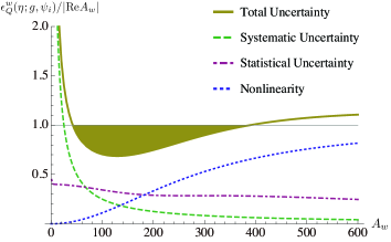
Figure 1: Ratio of uncertainty $\epsilon^{w}_{Q}(\eta;g,d)$ to the real part of the weak value of the spin $S_{z}=\sigma_{z}/2$. By amplifying the weak value out of its numerical range $[-1/2,1/2]$ to $(S_{z})_{w}\approx 100$, the significance condition (15) is attained with confidence $\eta=0.95$. (Parameters: $\delta_{Q}=1/2$, $N_{0}=10^{7}$, $g=1/50$ and $d=4$.)

Note, however, that the advantage of amplification does not come free, because the amplification requires generically a small transition amplitude $\langle\phi_{f}|\phi_{i}\rangle$, which necessitate a much larger number of prepared samples to suppress the statistical uncertainty compared to the conventional one. More importantly, the amplification enhances also the uncertainty coming from the nonlinearity and, together with the statistical uncertainty, eventually ruins the significance condition (15). In fact, it can be proved that, for an observable $A$ with finite eigenvalues, the shifts $\Delta^{w}_{X}(g)$ for fixed $g$ and $|\psi_{i}\rangle$ are also bounded with respect to a set of pre and postselections of the system and, as a result, the ratio between the amplified weak value and the nonlinear term becomes unity as $|\mathrm{Re}A_{w}|,\ |\mathrm{Im}A_{w}|\to\infty$, suggesting that the qualitative behaviour seen in this specific numerical demonstration is actually universal. Given these trade-offs, for probing a physical effect such as gravitational waves by means of weak measurement, it is vital for us to find a possible range of amplification fulfilling (15) where the measurement is significant.

- (1) Y. Aharonov, P. G. Bergmann and L. Lebowitz, Phys. Rev. 134 (1964) B1410.
- (2) Y. Aharonov, D. Z. Albert, and L. Vaidman, Phys. Rev. Lett. 60 (1988) 1351.
- (3) Y. Aharonov Y, and L. Vaidman, J. Phys. A: Math. Gen. 24 (1991) 2315.
- (4) K. Yokota, T. Yamamoto, M. Koashi and N. Imoto, New Journ. Phys. 11 (2009) 033011.
- (5) O. Hosten and P. Kwiat, SCIENCE 319 (2008) 787.
- (6) P. B. Dixon, D. J. Starling, A. N. Jordan, and J. C. Howell, Phys. Rev. Lett. 102 (2009) 173601.
- (7) S. Wu, and Y. Li, Phys. Rev. A 83 (2011) 052106.
- (8) R. Josza, Phys. Rev. A 76 (2007) 044103.
- (9) T. Koike and S. Tanaka, Phys. Rev. A 84, 062106 (2011).
- (10) K. Nakamura, A. Nishizawa, and M. K. Fujimoto, Phys. Rev. A 85, 012113 (2012).
- (11) Y. Susa, Y. Shikano, and A. Hosoya, Phys. Rev. A 85, 052110 (2012).
- (12) Y. Aharonov and D. Rohrlich, “Quantum Paradoxes: Quantum Theory for the Perplexed”, Wiley-VCH, Weinheim (2005).
- (13) S. Kocsis, B. Braverman, S. Ravets, M. J. Stevens, R. P. Mirin, L. K. Shalm and A. M. Steinberg, SCIENCE 332 (2011) 1170.
- (14) A. M. Steinberg Phys. Rev. Lett. 74 (1995) 2405.
- (15) J. Dressel, S. Agarwal, and A. N. Jordan, Phys. Rev. Lett. 104 (2010) 240401; J. Dressel and A. N. Jordan, Phys. Rev. A 85 (2012) 022123.
- (16) B. Reznik and Y. Aharonov, Phys. Rev. A 52 (1995) 2538.
- (17) Y. Aharonov, S. Popescu, J. Tollaksen and L. Vaidman, Phys. Rev. A 79 (2009) 052110.
- (18) T. Mark Beasley et al., Appl. Statist. 53, Part 1 (2004), pp. 95-108.