Parallel in time algorithm with spectral-subdomain enhancement for Volterra integral equations

Abstract.

This paper proposes a parallel in time (called also time parareal) method to solve Volterra integral equations of the second kind. The parallel in time approach follows the same spirit as the domain decomposition that consists of breaking the domain of computation into subdomains and solving iteratively the sub-problems in a parallel way. To obtain high order of accuracy, a spectral collocation accuracy enhancement in subdomains will be employed. Our main contributions in this work are two folds: (i) a time parareal method is designed for the integral equations, which to our knowledge is the first of its kind. The new method is an iterative process combining a coarse prediction in the whole domain with fine corrections in subdomains by using spectral approximation, leading to an algorithm of very high accuracy; (ii) a rigorous convergence analysis of the overall method is provided. The numerical experiment confirms that the overall computational cost is considerably reduced while the desired spectral rate of convergence can be obtained.

1. Introduction

We consider the linear Volterra integral equations (VIEs) of the second kind

(1.1) $${u}(t)-\int_{0}^{t}K(t,s){u}(s){\mathrm{d}}s=g(t),\qquad\forall t\in I:=[0,T],$$

where $g$ and $K$ are sufficiently smooth in $I$ and $I\times I$, respectively; and $K(t,t)\neq 0$ for all $t\in I$. Under these assumptions, smooth solution $u(t)$ to (1.1) exists and unique, see, e.g., [3].

The presence of the integral in (1.1) makes the problem globally time-dependent. This means that the solution at time $t_{k}$ depends on the solutions at all previous time $t<t_{k}$. Consequently, it may require large storage if the solution time is large or high accuracy of approximations is needed. This may become more serious if partial integro-differential equations are considered. To handle this, we will design our method by breaking the domain into sub-domains (as in the domain decomposition approach) and then solving iteratively the sub-problems in parallel way. More precisely, we divide the time interval $[0,T]$ into $N$ equi-spaced subintervals and then break the original problem into a series of independent problems on the small sub-intervals. These independent problems are solved by a fine approximation which can be implemented in a parallel way, together with some coarse grid approximations which have to be implemented in a sequential way.

The parallel in time algorithm for a model ordinary differential equation (ODE) was initially introduced by Lions, Maday, and Turinici [14] for solving evolution problems in parallel. It can be interpreted as a predictor-corrector scheme [1, 2], which involves a prediction step based on a coarse approximation and a correction step computed in parallel based on a fine approximation. Even though the time direction seems intrinsically sequential, the combination of a coarse and a fine solution procedure has proven to allow for more rapid (convergent) solutions if parallel architectures are available. The parallel in time algorithm has received considerable attention over the past years, especially in the community of the domain decomposition methods [6], fluid and structure problems [7], the Navier-Stokes equations [8], quantum control problems [15], and so on. For the parallel in time method based on the finite difference scheme, the convergence analysis for an ODE problem was given in [9].

In our algorithm, we also build in a recent spectral method approach to obtain exponential rate of convergence, see [5, 19, 20]. The main advantage of using high order methods for integral equations is their low storage requirement with the desired precision; this advantage makes high order methods attractive. Among the high order methods spectral methods are known very useful due to its exponential rate of convergence, which is also demonstrated for solving VIEs [18, 13]. However, a drawback of the spectral method is also well-known; i.e., the matrix associated with the spectral method is full and the computational cost grows more quickly than that of a low order method. Thus for long integration it is desirable to combine the spectral method with domain decomposition techniques to avoid using a single high-degree polynomials.

It is noted that there have been great interests in studying the parabolic integro-differential equations, in particular the study of discontinuous-Galerkin methods, see, e.g., [10, 17]. These studies are very relevant to the present study and it will be interesting to extend the present study to parabolic integro-differential equations. Another class of relevant problems is about space-time fractional diffusion equation which have been extensively studied [11, 12]. It is noted that the problems mentioned above also contain a weakly singular kernel in the memory term, which can provide extra difficulties in convergence analysis, see, e.g., the recent work on the spectral methods for VIEs with a weakly singular kernel [5, 13].

This paper is the first attempt to approximate solutions of the VIEs by the parallel in time method. In addition, this article will provide a full convergence analysis for the proposed method. We will also demonstrate numerically the efficiency and the convergence of the proposed method on some sample problems.

This paper is organized as follows. In section 2, we construct the parallel in time method based on the spectral collocation scheme for the underlying equation, and outline the main results. Some lemmas useful for the convergence analysis are provided in section 3. The convergence analysis for the proposed method in $L^{\infty}$ under some assumptions is given in section 4. Numerical experiments are carried out in section 5. In the final section we analyze the parallelism efficiency of the overall algorithm, together with a description of some implementation details.

2. Outline of the Parallem in Time Method and the Main Results

The time interval $I=[0,T]$ is first partitioned into $N$ subintervals, determined by the grid points $0=t_{0}<t_{1}<t_{2}<\cdots<t_{N}=T$ with $t_{n}=n\Delta t,\Delta t={T}/{N}$. We denote this partition by $I=\cup_{n=1}^{N}I_{n}$ with $I_{n}=[t_{n-1},t_{n}]$.

2.1. Outline of the method

In the obvious way, the problem (1.1) is equivalent to the following system of $N$ integral equations:

(2.1) $$u_{n}(t)-K_{nn}u_{n}(t)=g(t)+\sum^{n-1}_{j=1}K_{nj}u_{j}(t),\quad{\rm on}\;\;I_{n}=[t_{n-1},t_{n}],\ 1\leq n\leq N.$$

with $u_{j}=u|_{I_{j}}$,

(2.2) $$K_{nn}u_{n}(t):=\int^{t}_{t_{n-1}}K(t,s)u_{n}(s)ds,\;\;\;{\rm and}\;\;K_{nj}u_{j}(t):=\int^{t_{j}}_{t_{j-1}}K(t,s)u_{j}(s)ds,\;\;1\leq j\leq n-1.$$

The solution of (2.1) can be expressed through the solution operators $\mathcal{S}_{n}$ as follows:

(2.3) $$u_{n}(t)=\mathcal{S}_{n}(t;u_{1},\cdots,u_{n-1})\;\;{\rm for}\;t\in I_{n}.$$

Likewise, at the discrete level, we have the solution operators $\mathcal{F}_{n}$ for the collocation method to be described later:

(2.4) $$U_{n}(t)=\mathcal{F}_{n}(t;U_{1},\cdots,U_{n-1})\;\;{\rm for}\;t\in I_{n}.$$

with $U_{n}$ a polynomial of degree $M$. The main idea of the proposed parallel in time method is to take a second family of discrete solution operators, $\mathcal{G}_{n}$, defined in the same way using polynomials of a lower degree $\tilde{M}<M$, and to set up the iteration:

(2.5) $$U^{k}_{n}(t)=\mathcal{G}_{n}(t;U^{k}_{1},\cdots,U^{k}_{n-1})+\mathcal{C}_{n}(t;U^{k-1}_{1},\cdots,U^{k-1}_{n-1}),\;\;k\geq 1,$$

with the initial value

$$U^{0}_{n}=\mathcal{G}_{n}(t;U^{0}_{1},\cdots,U^{0}_{n-1}),$$

where the correction term in (2.5) is defined by

(2.6) $$\mathcal{C}_{n}(t;U^{k-1}_{1},\cdots,U^{k-1}_{n-1}):=\mathcal{F}_{n}(t;U^{k-1}_{1},\cdots,U^{k-1}_{n-1})-\mathcal{G}_{n}(t;U^{k-1}_{1},\cdots,U^{k-1}_{n-1}).$$

Here, the key is that the $\mathcal{C}_{n}$ can be computed in parallel for $1\leq n\leq N$. The term $\mathcal{G}_{n}$ in (2.5) must be computed sequentially, but this is relatively cheap if $\tilde{M}$ is small compared to $M$. Thus, provided the iteration converges rapidly, we can use multiple processors to obtain a high accuracy solution in a small multiple of the time needed to compute a low accuracy (sequential) solution.

It is pointed out that the way of presenting the parallel in time method places it in the category of the predictor-corrector scheme, where the predictor is $\mathcal{G}_{n}(t,U_{1}^{k},\cdots,U_{n-1}^{k})$ while the corrector is $\mathcal{C}_{n}(t;U^{k-1}_{1},\cdots,U^{k-1}_{n-1})$.

2.2. Outline of the main results

The main result of this paper will be the following:

(2.7) $$\|u_{n}-U^{k}_{n}\|_{\infty}=O(M^{3/4-m}+(\tilde{M}/2)^{(3/4-m)(k+1)}),$$

and numerical experiments confirm this convergence behavior in practice. Thus $U^{k}_{n}$ is accurate to $O(M^{3/4-m})$ if $M\approx(\tilde{M}/2)^{k+1}$. We emphasize that the analysis covers a fully-discrete scheme in which quadratures are used to approximate the integrals that occur in the coefficients and right-hand side of the resulting linear system that must be solved at the $n$-th interval to compute $U^{k}_{n}$.

2.3. The operators $\mathcal{F}_{n}$ and $\mathcal{G}_{n}$

We begin by discussing the operator $\mathcal{F}_{n}$ defined in (2.4). In this work, we will use a spectral collocation method to define this approximation. Define $\mathcal{P}_{M}(I_{n})$ as the polynomial spaces of degree less than or equal to $M$, with $I_{n}=[t_{n-1},t_{n}]$. Denote $L_{M}(x)$ the Legendre polynomial of degree $M$. Let $x_{i}$ be the points of the Legendre-Gauss (LG) quadrature formula, defined by $L_{M+1}(x_{i})=0,i=0,\cdots,M$, arranged by increasing order. The associated weights of the LG quadrature formula are denoted by $\omega_{i}$, $0\leq i\leq M$. Then it is well-known the following identity:

$$\int_{-1}^{1}\varphi(x){\mathrm{d}}x=\sum^{M}_{i=0}\varphi(x_{i})\omega_{i},\;\;\;\forall\varphi\in\mathcal{P}_{2M+1}(-1,1).$$

The discrete $L^{2}$ inner product associated to the LG quadrature is denoted by:

(2.8) $$(\varphi,\psi)_{M}:=\sum^{M}_{i=0}\varphi(x_{i})\psi(x_{i})\omega_{i}.$$

Furthermore, define the LG points $\{\xi_{n}^{i}\}^{M}_{i=0}$ on the element $I_{n}=[t_{n-1},t_{n}]$, i.e.,

$$\xi_{n}^{i}=\frac{t_{n}-t_{n-1}}{2}x_{i}+\frac{t_{n}+t_{n-1}}{2},\quad 0\leq i\leq M,\ \ 1\leq n\leq N,$$

and the corresponding weights $\rho_{n}^{i}={\Delta t}\omega_{i}/2$. Then it holds

$$\int_{I_{n}}\varphi(x){\mathrm{d}}x=\sum^{M}_{i=0}\varphi(\xi_{n}^{i})\rho_{n}^{i},\quad\forall\varphi\in\mathcal{P}_{2M+1}(I_{n}),\;\;1\leq n\leq N.$$

We now use the Legendre-collocation method to determine the operator $\mathcal{F}_{n}$ in (2.4). More precisely, we want to find $U_{n}(t)\in\mathcal{P}_{M}(I_{n})$ with $1\leq n\leq N$ such that for all $0\leq i\leq M$,

(2.9) $$U_{n}(\xi_{n}^{i})-\displaystyle\int_{t_{n-1}}^{\xi_{n}^{i}}K(\xi_{n}^{i},s)U_{n}(s){\mathrm{d}}s=g(\xi_{n}^{i})+\sum^{n-1}_{j=1}{\displaystyle\int_{t_{j-1}}^{t_{j}}}K(\xi_{n}^{i},s)U_{j}(s){\mathrm{d}}s,\;\;1\leq n\leq N.$$

In the implementation, the integral terms on the left hand sides of (2.9) are evaluated by using the following Gauss quadrature:

(2.10) $$\int_{t_{n-1}}^{\xi_{n}^{i}}K(\xi_{n}^{i},s)U_{n}(s){\mathrm{d}}s=\int_{-1}^{1}\bar{K}(\xi_{n}^{i},s_{n}^{i})U_{n}(s_{n}^{i}){\mathrm{d}}x\thickapprox\left(\bar{K}(\xi_{n}^{i},s_{n}^{i}),U_{n}(s_{n}^{i})\right)_{M},$$

where $s_{n}^{i}:=s_{n}^{i}(x):=\frac{\xi_{n}^{i}-t_{n-1}}{2}x+\frac{\xi_{n}^{i}+t_{n-1}}{2},-1<x<1$, and

(2.11) $$\bar{K}(\xi_{n}^{i},s_{n}^{i}):=\left(\frac{\xi_{n}^{i}-t_{n-1}}{2}\right)K(\xi_{n}^{i},s_{n}^{i}).$$

The right-hand sides of (2.9) are computed in a similar way:

(2.12) $$\int_{t_{j-1}}^{t_{j}}K(\xi_{n}^{i},s)U_{j}(s){\mathrm{d}}s=\frac{\Delta t}{2}\int_{-1}^{1}K(\xi_{n}^{i},s_{j})U_{j}(s_{j}){\mathrm{d}}x\thickapprox\frac{\Delta t}{2}\left(K(\xi_{n}^{i},s_{j}),U_{j}(s_{j})\right)_{M},$$

where

(2.13) $$s_{j}=s_{j}(x)=\frac{\Delta t}{2}x+\frac{t_{j}+t_{j-1}}{2},\quad-1<x<1.$$

With the help of the above numerical integrations, (2.9) is further approximated by: $0\leq i\leq M$,

(2.14) $$U_{n}(\xi_{n}^{i})-\left(\bar{K}(\xi_{n}^{i},s_{n}^{i}),U_{n}(s_{n}^{i})\right)_{M}=g(\xi_{n}^{i})+{\triangle t\over 2}\sum^{n-1}_{j=1}\left(K(\xi_{n}^{i},s_{j}),U_{j}(s_{j})\right)_{M},\;\;1\leq n\leq N.$$

The above linear system defines the fine operator $\mathcal{F}_{n}$ in (2.4).

The operator $\mathcal{G}_{n}$ is defined by the same spectral collocation method but with the degree $\tilde{M}$, which is much less than $M$.

Let $\{\eta_{n}^{i}\}_{i=0}^{\tilde{M}}$ be a set of LG-points on the element $[t_{n-1},t_{n}]$ corresponding to the weight $\{\varrho_{n}^{i}\}_{i=0}^{\tilde{M}}$. Then the coarse operator $\mathcal{G}_{n}(t,V_{1},\cdots,V_{n-1})$ in (2.5) consists in finding $V_{n}(t)\in\mathcal{P}_{\tilde{M}}(I_{n})$, such that, for all $0\leq i\leq\tilde{M}$

(2.15) $$V_{n}(\eta_{n}^{i})-\left(\bar{K}(\eta_{n}^{i},\tau_{n}^{i}),V_{n}(\tau_{n}^{i})\right)_{\tilde{M}}=g(\eta_{n}^{i})+{\Delta t\over 2}\sum^{n-1}_{j=1}\left(K(\eta_{n}^{i},s_{j}),V_{j}(s_{j})\right)_{\tilde{M}},\quad 1\leq n\leq N,$$

where $\tau_{n}^{i}:=\tau_{n}^{i}(x):=\frac{\eta_{n}^{i}-t_{n-1}}{2}x+\frac{\eta_{n}^{i}+t_{n-1}}{2},\ -1<x<1,$ and $\bar{K}$ and $s_{j}$ are respectively defined in (2.11) and (2.13).

3. Useful Lemmas

We first introduce some notations. Let $\Lambda$ be an arbitrary bounded interval. For non-negative integer $m$, $H^{m}(\Lambda)$ stands for the standard Sobolev space equipped with the norm and seminorm $\|v\|_{m,\Lambda}$ and $|v|_{k,\Lambda},0\leq k\leq m$. Particularly $L^{2}(\Lambda)=H^{0}(\Lambda)$, equipped with the standard $L^{2}$-inner product and norm. Similarly, the norm of the space $W^{m,\infty}(\Lambda)$ is denoted by $\|v\|_{W^{m,\infty}(\Lambda)}$ or $\|v\|_{\infty,\Lambda}$ if $m=0$. The error analysis needs the following seminorm:

$$|v|_{H^{m;M}(\Lambda)}=\left(\sum_{k=\min(m,M+1)}^{m}\|\partial_{x}^{(k)}v\|_{\Lambda}^{2}\right)^{\frac{1}{2}}.$$

Hereafter, in cases where no confusion would arise, the domain symbol $\Lambda$ may be dropped from the notations. We denote by $c$ generic positive constants independent of the discretization parameters, but may depend on the kernel function $K(\cdot,\cdot)$ or $T$.

We further introduce two approximation operators. Firstly, we define the Lagrange interpolation operator $\mathcal{I}_{\Lambda}^{M}:\ \mathcal{C}(\Lambda)\rightarrow\mathcal{P}_{M}(\Lambda)$, by: $\forall v\in\mathcal{C}({\Lambda}),\mathcal{I}_{\Lambda}^{M}v\in\mathcal{P}_{M}(\Lambda)$, such that

$$\mathcal{I}_{\Lambda}^{M}v(z_{i})=v(z_{i}),\quad 0\leq i\leq M,$$

where $\{z_{i}\}_{i=0}^{M}$ is the set of LG-points on the interval $\Lambda$. This polynomial can be expressed as

$$\mathcal{I}_{\Lambda}^{M}v(x)=\sum_{i=0}^{M}v(z_{i})h_{\Lambda}^{i}(x),$$

where $h_{\Lambda}^{i}$ is the Lagrange interpolation basis function associated with $\{z_{i}\}_{i=0}^{M}$. Particularly, we use $\mathcal{I}_{n}^{M}$ (resp., $h_{n}^{i}(x)$) to replace $\mathcal{I}_{\Lambda}^{M}$ (resp., $h_{\Lambda}^{i}(x)$) when $\Lambda=I_{n}$.

Then for all $v\in H^{m}(\Lambda),m\geqslant 1$, the following optimal error estimates hold (see, e.g., [4, 18]):

(3.1) $$\|v-\mathcal{I}_{\Lambda}^{M}v\|\lesssim M^{-m}|v|_{H^{m;M}},$$

(3.2) $$\|v-\mathcal{I}_{\Lambda}^{M}v\|_{\infty}\lesssim M^{\frac{3}{4}-m}|v|_{H^{m;M}}.$$

For the discrete $L^{2}$-inner product defined in (2.8), it holds the following error estimate [4]:  $\forall\phi\in\mathcal{P}_{M}(\Lambda)$,

(3.3) $$|(v,\phi)-(v,\phi)_{M}|\lesssim M^{-m}|v|_{H^{m;M}}\|\phi\|,\ \ v\in H^{m}(\Lambda),\ \ m\geq 1.$$

The following result gives the Lebesgue constant for the Lagrange interpolation polynomials associated with the LG-points.

Lemma 3.1.

(p.329, eq.(9) in [16]) Let $\{h_{\Lambda}^{j}(x)\}_{j=0}^{M}$ be the Lagrange interpolation basis associated with the $M+1$ LG-points on the interval $\Lambda$. Then

(3.4) $$\|I_{\Lambda}^{M}\|_{\infty}:=\max_{x\in\Lambda}\sum_{j=0}^{M}|h_{\Lambda}^{j}(x)|\lesssim\sqrt{M}.$$

Using the standard Gronwall inequality, we obtain the following estimate for the Volterra integral equations.

Lemma 3.2.

Consider the following Volterra equation:

(3.5) $$u(t)=v(t)+\int_{0}^{t}K(t,s)u(s){\mathrm{d}}s.$$

If $v\in W^{m,\infty}$ and $K(t,s)$ is sufficiently smooth, then

(3.6) $$\left\|u\right\|_{W^{m,\infty}}\leq c2^{m}\left\|v\right\|_{W^{m,\infty}}.$$

Proof.

It is known (see, e.g., [3]) that there exists a smooth resolvent kernel $R(t,s)$ depending only on $K(t,s)$ such that the solution of (3.6) satisfies

$$u(t)=v(t)+\int^{t}_{0}R(t,s)v(s)ds.$$

Using the transformation $\tau=s/t$ leads to

$$u(t)=v(t)+\int^{1}_{0}tR(t,t\tau)v(t\tau)d\tau.$$

Differentiating the above equation with respect to $t$ $m$-times gives

$$u^{(m)}(t)=v^{(m)}(t)+\sum^{m}_{j=0}C^{j}_{m}\int^{1}_{0}\partial^{(m-j)}_{t}(tR(t,t\tau))v^{(j)}(t\tau)\tau^{j}d\tau,$$

which leads to

$$\|u^{(m)}\|\leq\|v^{(m)}\|+c\sum^{m}_{j=0}C^{j}_{m}\int^{1}_{0}\tau^{j}d\tau\|v^{(m)}\|\leq c2^{m}\|v^{(m)}\|,$$

where the constsnt $c$ depends on the regularity of $R$, or quivalently the regularity of $K$. This completes the proof of the lemma. ∎

We also need the following discrete Gronwall lemma (see, e.g., [3]).

Lemma 3.3.

Assume that $\phi_{n},p_{n}$ and $k_{n}$ are three sequences, $k_{n}$ is non-negative, and they satisfy

$$\left\{\begin{array}[]{l}\phi_{0}\leq g_{0},\\ \phi_{n}\leq g_{0}+\sum\limits_{s=0}^{n-1}p_{s}+\sum\limits_{s=0}^{n-1}k_{s}\phi_{s},\ \ n\geq 1.\end{array}\right.$$

Then it holds

$$\left\{\begin{array}[]{l}\phi_{1}\leq g_{0}(1+k_{0})+p_{0}\\ \phi_{n}\leq g_{0}\prod\limits_{s=0}^{n-1}(1+k_{s})+\sum\limits_{s=0}^{n-2}p_{s}\prod\limits_{\tau=s+1}^{n-1}(1+k_{r})+p_{n-1},\ \ n\geq 2.\end{array}\right.$$

Moreover, if $g_{0}\geq 0$ and $p_{n}\geq 0$ for all $n\geq 0$, then it holds

$$\phi_{n}\leq\left(g_{0}+\sum_{s=0}^{n-1}p_{s}\right)\exp\left(\sum_{s=0}^{n-1}k_{s}\right),\ \ n\geq 1.$$

4. Stability and Convergence Analysis

This section is devoted to the stability and convergence analysis of the proposed parallel in time scheme.

4.1. Stability

Lemma 4.1.

For $1\leq n\leq N$, let $\mathcal{F}_{n}$ be the fine approximation operator defined by the spectral collocation scheme (2.14), $\mathcal{G}_{n}$ defined by (2.15), $g_{M}=\mathcal{I}_{n}^{M}g$, and $\{\psi_{i}\}_{i=1}^{n-1}$ be a polynomial sequence. Then for sufficiently large $M$ and $\tilde{M}$ we have

(4.1) $$\left\|\mathcal{F}_{n}(t;\psi_{1},\cdots,\psi_{n-1})\right\|_{\infty}\leq c\Big{(}\|g_{M}\|_{\infty}+\Delta t\sum^{n-1}_{j=1}\|\psi_{j}\|_{\infty}\Big{)},$$

(4.2) $$\left\|\mathcal{G}_{n}(t;\psi_{1},\cdots,\psi_{n-1})\right\|_{\infty}\leq c\Big{(}\|g_{\tilde{M}}\|_{\infty}+\Delta t\sum^{n-1}_{j=1}\|\psi_{j}\|_{\infty}\Big{)},\;\;\;n\geq 1,$$

where it is understood that $\mathcal{F}_{1}(t;\psi_{0}):=\mathcal{F}_{1}(t)$ and $\mathcal{G}_{1}(t;\psi_{0}):=\mathcal{G}_{1}(t)$.

Proof.

Since the only difference between $\mathcal{F}_{n}$ and $\mathcal{G}_{n}$ is the polynomial degree, we only need to prove (4.1). Let $\psi_{n}:=\mathcal{F}_{n}(t;\psi_{1},\cdots,\psi_{n-1})$. It follows from the spectral collocation scheme (2.14) that

(4.3) $$\psi_{n}(\xi_{n}^{i})=g(\xi_{n}^{i})+\left(\bar{K}(\xi_{n}^{i},s_{n}^{i}),\psi_{n}(s_{n}^{i})\right)_{M}+\frac{\Delta t}{2}\sum^{n-1}_{j=0}\left(K(\xi_{n}^{i},s_{j}),\psi_{j}(s_{j})\right)_{M},\ 0\leq i\leq M,$$

which can be further re-organized as

(4.4) $$\psi_{n}(\xi_{n}^{i})=g(\xi_{n}^{i})+\left(\bar{K}(\xi_{n}^{i},s_{n}^{i}),\psi_{n}(s_{n}^{i})\right)+A^{i}_{n}+\frac{\Delta t}{2}\sum^{n-1}_{j=1}\left(K(\xi_{n}^{i},s_{j}),\psi_{j}(s_{j})\right)+\sum^{n-1}_{j=1}A^{i}_{j},$$

where

$$A_{n}^{i}=-\left(\bar{K}(\xi_{n}^{i},s_{n}^{i}),\psi_{n}(s_{n}^{i})\right)+\left(\bar{K}(\xi_{n}^{i},s_{n}^{i}),\psi_{n}(s_{n}^{i})\right)_{M},$$

$$A_{j}^{i}=-\frac{\Delta t}{2}\left(K(\xi_{n}^{i},s_{j}),\psi_{j}(s_{j})\right)+\frac{\Delta t}{2}\left(K(\xi_{n}^{i},s_{j}),\psi_{j}(s_{j})\right)_{M},\quad 1\leq j\leq n-1.$$

Multiplying both sides of (4.4) by the Lagrange basis function $h_{n}^{i}$ and summing up from $i=0$ to $i=M$, we obtain

$$\psi_{n}(t) = \mathcal{I}_{n}^{M}g+\mathcal{I}_{n}^{M}\int_{t_{n-1}}^{t}K(t,s)\psi_{n}(s){\mathrm{d}}s+\sum_{i=0}^{M}A_{n}^{i}h_{n}^{i}(t)$$

$$\;\;\;+\sum^{n-1}_{j=1}\Big{[}\frac{\Delta t}{2}\mathcal{I}_{n}^{M}\left(K(t,s_{j}),\psi_{j}(s_{j})\right)+\sum_{i=0}^{M}A_{j}^{i}h_{j}^{i}(t)\Big{]}.$$

Consequently, we have

(4.6) $$\psi_{n}(t)=\int_{t_{n-1}}^{t}K(t,s)\psi_{n}(s){\mathrm{d}}s+\mathcal{I}_{n}^{M}g+\sum_{j=1}^{n}J_{j}+\sum_{j=1}^{n}I_{j}+\sum_{j=1}^{n-1}R_{j},$$

where

$$J_{j}=\sum\limits_{i=0}^{M}A_{j}^{i}h_{j}^{i},\quad 1\leq j\leq n,$$

$$I_{n}=\mathcal{I}_{n}^{M}\left(\bar{K}(t,s_{n}^{i}),\psi_{n}(s_{n}^{i})\right)-\left(\bar{K}(t,s_{n}^{i}),\psi_{n}(s_{n}^{i})\right),$$

$$I_{j}=\frac{\Delta t}{2}\mathcal{I}_{n}^{M}\left(K(t,s_{j}),\psi_{j}(s_{j})\right)-\frac{\Delta t}{2}\left(K(t,s_{j}),\psi_{j}(s_{j})\right),\quad 1\leq j\leq n-1,$$

$$R_{j}=\frac{\Delta t}{2}\left(K(t,s_{j}),\psi_{j}(s_{j})\right),\quad 1\leq j\leq n-1.$$

It follows from the standard Gronwall inequality for (4.6) that

(4.7) $$\|\psi_{n}\|_{\infty}\leq c\left(\|g_{M}\|_{\infty}+\sum_{j=1}^{n}\|J_{j}\|_{\infty}+\sum_{j=1}^{n}\|I_{j}\|_{\infty}+\sum_{j=1}^{n-1}\|R_{j}\|_{\infty}\right).$$

We now estimate the right hand-side of (4.7) term by term. First, we estimate the terms $J_{j}$. Using the error estimate (3.3) for the LG-quadrature, we have

$$\max_{0\leq i\leq M}|A_{n}^{i}| = \max_{0\leq i\leq M}\left|\left(\bar{K}(\xi_{n}^{i},s_{n}^{i}),\psi_{n}(s_{n}^{i})\right)_{M}-\int_{t_{n-1}}^{\xi_{n}^{i}}K(\xi_{n}^{i},s)\psi_{n}(s){\mathrm{d}}s\right|$$

$$\leq c\Delta tM^{-1}\max_{0\leq i\leq M}|K(\xi_{n}^{i},s_{n}^{i})|_{H^{1;M}}\max_{0\leq i\leq M}\|\psi_{n}(s_{n}^{i})\|$$

$$\leq c_{1}\Delta tM^{-1}\|\psi_{n}\|_{\infty},$$

where $c_{1}$ depends on $|K(\xi_{n}^{i},s_{n}^{i}(\cdot))|_{H^{1;M}}$. Similarly,

(4.9) $$\max_{0\leq i\leq M}|A_{j}^{i}|\leq c_{1}\Delta tM^{-1}\|\psi_{j}\|_{\infty},\quad 1\leq j\leq n-1.$$

Hence, combining (4.1) and (4.9) with Lemma 3.1 gives

$$\|J_{n}\|_{\infty}=\left\|\sum_{i=0}^{M}A_{n}^{i}h_{n}^{i}\right\|_{\infty}\leq\max_{0\leq i\leq M}|A_{n}^{i}|\max_{x\in I_{n}}\sum_{i=0}^{M}|h_{n}^{i}|\leq c_{1}\Delta tM^{-\frac{1}{2}}\|\psi_{n}\|_{\infty}\leq\frac{1}{3c}\|\psi_{n}\|_{\infty}$$

for sufficiently small $\Delta t$ or large $M$. Following the same lines leads to

(4.10) $$\|J_{j}\|_{\infty}\leq c_{1}\Delta tM^{-\frac{1}{2}}\|\psi_{j}\|_{\infty},\quad 1\leq j\leq n-1.$$

We now estimate the second term $I_{j}$. For $j=n$, applying (3.2) leads to

$$\left\|I_{n}\right\|_{\infty} = \left\|(\mathcal{I}_{n}^{M}-\mathcal{I})\int_{t_{n-1}}^{t}K(t,s)\psi_{n}(s){\mathrm{d}}s\right\|_{\infty}\leq c_{1}M^{-\frac{1}{4}}\left|\int_{t_{n-1}}^{t}K(t,s)\psi_{n}(s){\mathrm{d}}s\right|_{H^{1;M}}$$

$$\leq c_{1}M^{-\frac{1}{4}}\|\psi_{n}\|_{\infty}\leq\frac{1}{3c}\|\psi_{n}\|_{\infty}.$$

For $1\leq j\leq n-1$, in virtue of (3.2), we derive

$$\left\|I_{j}\right\|_{\infty} = \left\|(\mathcal{I}_{n}^{M}-\mathcal{I})\int_{t_{j-1}}^{t_{j}}K(t,s)\psi_{j}(s){\mathrm{d}}s\right\|_{\infty}\leq c_{1}M^{\frac{3}{4}-1}\left|\int_{t_{j-1}}^{t_{j}}K(t,s)\psi_{j}(s){\mathrm{d}}s\right|_{H^{1;M}}$$

$$\leq c_{1}\Delta tM^{-\frac{1}{4}}\left\|\psi_{j}\right\|_{\infty}.$$

It remains to estimate $R_{j}$. By a direct calculation, we have

(4.12) $$\|R_{j}\|_{\infty}=\frac{\Delta t}{2}\left\|\left(K(t,s_{j}),\psi_{j}(s_{j})\right)\right\|_{\infty}\leq c\Delta t\|\psi_{j}\|_{\infty},\quad 1\leq j\leq n-1.$$

Finally, combining (4.7)-(4.12) gives

$$\|\psi_{n}\|_{\infty} \leq c\|g_{M}\|_{\infty}+\frac{1}{3}\|\psi_{n}\|_{\infty}+c\Delta tM^{-\frac{1}{2}}\sum^{n-1}_{j=1}\|\psi_{j}\|_{\infty}$$

$$+\frac{1}{3}\|\psi_{n}\|_{\infty}+c\Delta tM^{-\frac{1}{4}}\sum^{n-1}_{j=1}\left\|\psi_{j}\right\|_{\infty}+c\Delta t\sum^{n-1}_{j=1}\|\psi_{j}\|_{\infty}.$$

Now a simple rearrangement leads to (4.1). ∎

We are now ready to state and prove one of the main results of this paper.

Theorem 4.1.

(Stability) The iteration scheme (2.5)-(2.6) is stable in the sense that the solution $U_{n}^{k}$ satisfies

(4.14) $$\|U_{n}^{k}\|_{\infty}\leq c\|g_{\tilde{M}}\|_{\infty},\;\;\;\forall k\geq 0,\;\;1\leq n\leq N.$$

Proof.

For $k=0$, it follows from the initial value $U^{0}_{n}=\mathcal{G}_{n}(t;U^{0}_{1},\cdots,U^{0}_{n-1})$ and Lemma 4.1 that

(4.15) $$\|U_{n}^{0}\|_{\infty}=\left\|\mathcal{G}_{n}\left(t,U_{1}^{0},\cdots,U_{n-1}^{0}\right)\right\|_{\infty}\leq c_{0}\Big{(}\|g_{\tilde{M}}\|_{\infty}+\Delta t\sum^{n-1}_{j=1}\|U_{j}^{0}\|_{\infty}\Big{)}.$$

By applying the discrete Gronwall Lemma 3.3, we get

(4.16) $$\|U_{n}^{0}\|_{\infty}\leq c_{0}e^{c_{0}(n-1)\Delta t}\|g_{\tilde{M}}\|_{\infty}\leq c_{0}e^{c_{0}T}\|g_{\tilde{M}}\|_{\infty}.$$

For $k\geq 1$, according to the iteration scheme (2.5)-(2.6), we have

(4.17) $$\|U_{n}^{k}\|_{\infty} \leq \left\|\mathcal{G}_{n}\left(t;U_{1}^{k},U_{2}^{k},\cdots,U_{n-1}^{k}\right)\right\|_{\infty}$$

$$+\left\|\mathcal{F}_{n}\left(t;U_{1}^{k-1},U_{2}^{k-1},\cdots,U_{n-1}^{k-1}\right)\right\|_{\infty}+\left\|\mathcal{G}_{n}\left(t;U_{1}^{k-1},U_{2}^{k-1},\cdots,U_{n-1}^{k-1}\right)\right\|_{\infty}.$$

Applying Lemma 4.1 to the right hand side of (4.17) yields

(4.18) $$\|U_{n}^{k}\|_{\infty} \leq c\Big{(}\|g_{\tilde{M}}\|_{\infty}+\Delta t\sum^{n-1}_{j=1}\|U_{j}^{k}\|_{\infty}\Big{)}+c\Big{(}\|g_{\tilde{M}}\|_{\infty}+\|g_{M}\|_{\infty}+\Delta t\sum^{n-1}_{j=1}\|U_{j}^{k-1}\|_{\infty}\Big{)}$$

$$\leq c_{0}\Delta t\sum^{n-1}_{j=1}\|U_{j}^{k}\|_{\infty}+c\Big{(}\|g_{\tilde{M}}\|_{\infty}+\Delta t\sum^{n-1}_{j=1}\|U_{j}^{k-1}\|_{\infty}\Big{)}.$$

In the following, we will derive the following inequality

(4.19) $$\|U_{n}^{k}\|_{\infty}\leq c_{0}\sum_{l=0}^{k}\frac{e^{c_{0}(l+1)(n-1)\Delta t}}{l!}\|g_{\tilde{M}}\|_{\infty},\ \ \forall k\geq 0,1\leq n\leq N,$$

where $c_{0}$ is a constant independent of $k$. We do this by induction. First, it follows from (4.16) that (4.19) is true for $k=0$. We now show that if (4.19) holds for a given $k$ then it also holds for $k+1$. It follows from (4.18) (replace $k$ by $k+1$) and the discrete Gronwall Lemma 3.3 that

(4.20) $$\|U_{n}^{k+1}\|_{\infty}\leq c_{0}e^{c_{0}(n-1)\Delta t}\left(\|g_{\tilde{M}}\|_{\infty}+\Delta t\sum^{n-1}_{j=1}\|U_{j}^{k}\|_{\infty}\right).$$

Then using the induction assmption (4.19) gives

$$\|U_{n}^{k+1}\|_{\infty} \leq c_{0}\|g_{\tilde{M}}\|_{\infty}e^{c_{0}(n-1)\Delta t}\left(1+c_{0}\Delta t\sum_{l=0}^{k}\frac{e^{c_{0}(l+1)(n-2)\Delta t}}{l!}+\cdots+c_{0}\Delta t\sum_{l=0}^{k}\frac{1}{l!}\right)$$

$$= c_{0}\|g_{\tilde{M}}\|_{\infty}e^{c_{0}(n-1)\Delta t}\left(1+c_{0}\Delta t\sum_{l=0}^{k}\frac{1}{l!}\frac{e^{c_{0}(l+1)(n-1)\Delta t}-1}{e^{c_{0}(l+1)\Delta t}-1}\right)$$

$$\leq c_{0}\|g_{\tilde{M}}\|_{\infty}e^{c_{0}(n-1)\Delta t}\left(1+\sum_{l=0}^{k}\frac{1}{(l+1)!}(e^{c_{0}(l+1)(n-1)\Delta t}-1)\right)$$

$$\leq c_{0}\|g_{\tilde{M}}\|_{\infty}e^{c_{0}(n-1)\Delta t}\left(1+\sum_{l=0}^{k}\frac{1}{(l+1)!}e^{c_{0}(l+1)(n-1)\Delta t}\right)$$

$$\leq c_{0}\|g_{\tilde{M}}\|_{\infty}\sum_{l=0}^{k+1}\frac{e^{c_{0}(l+1)(n-1)\Delta t}}{l!}.$$

This implies that (4.19) also holds for $k$ being replaced by $k+1$. Finally, by noticing the fact that

(4.21) $$\sum_{l=0}^{\infty}\frac{e^{c_{0}(l+1)(n-1)\Delta t}}{l!}\leq e^{c_{0}(n-1)\Delta t}e^{e^{c_{0}(n-1)\Delta t}}\leq e^{c_{0}T}e^{e^{c_{0}T}},\ \ 1\leq n\leq N,$$

the desired result (4.14) follows from (4.19). ∎

Remark. It is seen from (4.19) and (4.21) that the generic constant $c$ in (4.14) has a rapid, double-exponential growth in $T$. Theoretically, this may become very large. On the other hand, our numerical experiemnts (see Section 5) can take $T=100$ without any apparent problem. It may be possible to obtain a better generic constant in (4.14), even by assuming something more on the kernel function $K(t,s)$. We believe that other proof techniques are needed to improve this double-exponential growth constant, and this is certainly an interesting theoretical challenge.

4.2. Convergence

We now provide an estimate for the fine approximation operator $\mathcal{F}_{n}$.

Lemma 4.2.

Let $u_{n}$ be the solution of (2.1) and $U_{n}$ be the solution of (2.4). If $u\in H^{m}(I),m\geq 1$, then we have

(4.22) $$\|u_{n}-U_{n}\|_{\infty}\leq c\left(M^{\frac{3}{4}-m}|u|_{H^{m;M}}+M^{\frac{1}{2}-m}\|u\|_{\infty}\right),\quad 1\leq n\leq N,$$

provided the number of collocation points $M$ is sufficiently large.

Proof.

Replace $t$ in (2.1) by $\zeta^{i}_{n}$. Subtracting the resulting equation from (2.14) gives

(4.23) $$u_{n}(\xi_{n}^{i})-U_{n}(\xi_{n}^{i})=\left(\bar{K}(\xi_{n}^{i},s_{n}^{i}),u_{n}(s_{n}^{i})\right)$$

$$\;\;\;-\left(\bar{K}(\xi_{n}^{i},s_{n}^{i}),U_{n}(s_{n}^{i})\right)_{M}+\frac{\Delta t}{2}\sum^{n-1}_{j=1}\Big{[}\left(K(\xi_{n}^{i},s_{j}),u_{j}(s_{j})\right)-\left(K(\xi_{n}^{i},s_{j}),U_{j}(s_{j})\right)_{M}\Big{]}.$$

It can be further re-organized as

$$u_{n}(\xi_{n}^{i})-U_{n}(\xi_{n}^{i})=\left(\bar{K}(\xi_{n}^{i},s_{n}^{i}),e_{n}(s_{n}^{i})\right)+A_{n}^{i}+\frac{\Delta t}{2}\sum^{n-1}_{j=1}\Big{[}\left(K(\xi_{n}^{i},s_{j}),e_{j}(s_{j})\right)+A^{i}_{j}\Big{]},$$

where $e_{j}:=u_{j}-U_{j}$,

$$A_{n}^{i}=\left(\bar{K}(\xi_{n}^{i},s_{n}^{i}),U_{n}(s_{n}^{i})\right)-\left(\bar{K}(\xi_{n}^{i},s_{n}^{i}),U_{n}(s_{n}^{i})\right)_{M},$$

$$A_{j}^{i}=\frac{\Delta t}{2}\left(K(\xi_{n}^{i},s_{j}),U_{j}(s_{j})\right)-\frac{\Delta t}{2}\left(K(\xi_{n}^{i},s_{j}),U_{j}(s_{j})\right)_{M},\quad 1\leq j\leq n-1.$$

Following the same procedure as in the proof of Lemma 4.1 gives

$$\mathcal{I}_{n}^{M}u_{n}-U_{n}=\mathcal{I}_{n}^{M}\left(\bar{K}(\xi_{n}^{i},s_{n}^{i}),e_{n}(s_{n}^{i})\right)+\sum_{i=0}^{M}A_{n}^{i}h_{n}^{i}+\sum^{n-1}_{j=1}\Big{[}\frac{\Delta t}{2}\mathcal{I}_{n}^{M}\left(K(\xi_{n}^{i},s_{j}),e_{j}(s_{j})\right)+\sum_{i=0}^{M}A_{j}^{i}h_{j}^{i}\Big{]}.$$

Consequently,

$$u_{n}-U_{n}=\int_{t_{n-1}}^{\xi_{n}^{i}}K(\xi_{n}^{i},s)e_{n}(s){\mathrm{d}}s+u_{n}-\mathcal{I}_{n}^{M}u_{n}+\sum_{j=1}^{n}J_{j}+\sum_{j=1}^{n}I_{j}+\sum_{j=1}^{n-1}R_{j},$$

where

$$J_{j}=\sum\limits_{i=0}^{M}A_{j}^{i}h_{j}^{i},\quad 1\leq j\leq n;\quad R_{j}=\frac{\Delta t}{2}\left(K(\xi_{n}^{i},s_{j}),e_{j}\right),\quad 1\leq j\leq n-1,$$

$$I_{n}=\mathcal{I}_{n}^{M}\left(\bar{K}(\xi_{n}^{i},s_{n}^{i}),e_{n}(s_{n}^{i})\right)-\left(\bar{K}(\xi_{n}^{i},s_{n}^{i}),e_{n}(s_{n}^{i})\right),$$

$$I_{j}=\frac{\Delta t}{2}\mathcal{I}_{n}^{M}\left(K(\xi_{n}^{i},s_{j}),e_{j}(s_{j})\right)-\frac{\Delta t}{2}\left(K(\xi_{n}^{i},s_{j}),e_{j}(s_{j})\right),\quad 1\leq j\leq n-1.$$

Applying the Gronwall Lemma 3.3 gives

(4.24) $$\|u_{n}-U_{n}\|_{\infty}\leq c\left(\left\|\mathcal{I}_{n}^{M}u_{n}-u_{n}\right\|_{\infty}+\sum_{j=1}^{n}\|J_{j}\|_{\infty}+\sum_{j=1}^{n}\|I_{j}\|_{\infty}+\sum_{j=1}^{n-1}\|R_{j}\|_{\infty}\right).$$

We now estimate the right-hand side of (4.24) term by term. First, it follows from the inequality (3.2) that

(4.25) $$\left\|\mathcal{I}_{n}^{M}u_{n}-u_{n}\right\|_{\infty}\leq cM^{\frac{3}{4}-m}|u_{n}|_{H^{m;M}}.$$

Then by using a similar technique as in the proof of Lemma 4.1, we can estimate $\|I_{j}\|_{\infty}$ and $\|J_{j}\|_{\infty}$ as follows. For $j=n$ and sufficiently large $M$,

(4.26) $$\|J_{n}\|_{\infty}=\left\|\sum\limits_{i=0}^{M}A_{n}^{i}h_{n}^{i}\right\|_{\infty}\!\leq c_{1}\Delta tM^{\frac{1}{2}-m}\Big{(}\|e_{n}\|_{\infty}+\|u_{n}\|_{\infty}\Big{)}\leq\frac{1}{3c}\|e_{n}\|_{\infty}+c\Delta tM^{\frac{1}{2}-m}\|u_{n}\|_{\infty},$$

where, as in Lemma 4.1, $c_{1}$, and therefore $c$, depend on $|K(\xi_{n}^{i},s_{n}^{i}(\cdot))|_{H^{m;M}}$. Similarly, we have

(4.27) $$\|I_{n}\|_{\infty}=\left\|\mathcal{I}_{n}^{M}\left(\bar{K}(\xi_{n}^{i},s_{n}^{i}),e_{n}(s_{n}^{i})\right)-\left(\bar{K}(\xi_{n}^{i},s_{n}^{i}),e_{n}(s_{n}^{i})\right)\right\|_{\infty}\leq\frac{1}{3c}\|e_{n}\|_{\infty}.$$

For $1\leq j\leq n-1$, we can further have

(4.28a) $$\|J_{j}\|_{\infty}=\left\|\sum\limits_{i=0}^{M}A_{j}^{i}h_{j}^{i}\right\|_{\infty}\leq c\Delta tM^{\frac{1}{2}-m}\Big{(}\|e_{j}\|_{\infty}+\|u_{j}\|_{\infty}\Big{)},$$

(4.28b) $$\|I_{j}\|_{\infty}=\frac{\Delta t}{2}\left\|\mathcal{I}_{n}^{M}\left(K(\xi_{n}^{i},s_{j}),e_{j}(s_{j})\right)-\left(K(\xi_{n}^{i},s_{j}),e_{j}(s_{j})\right)\right\|_{\infty}\leq c\Delta t\|e_{j}\|_{\infty},$$

(4.28c) $$\|R_{j}\|_{\infty}=\frac{\Delta t}{2}\left\|\left(K(t,s_{j}),e_{j}(s_{j})\right)\right\|_{\infty}\leq c\Delta t\|e_{j}\|_{\infty}.$$

Combining (4.24)-(4.28) yields

$$\|e_{n}\|_{\infty} \leq c\Big{(}M^{\frac{3}{4}-m}|u_{n}|_{H^{m;M}}+\frac{2}{3c}\|e_{n}\|_{\infty}+\Delta tM^{\frac{1}{2}-m}\|u_{n}\|_{\infty}\Big{)}$$

$$\;\;+c\Delta tM^{\frac{1}{2}-m}\sum^{n-1}_{j=1}\|u_{j}\|_{\infty}+c\Delta t\sum^{n-1}_{j=1}\|e_{j}\|_{\infty}.$$

Using the discrete Gronwall Lemma 3.3 gives

(4.29) $$\|e_{n}\|_{\infty}\leq c\left(M^{\frac{3}{4}-m}|u|_{H^{m;M}}+n\Delta tM^{\frac{1}{2}-m}\|u\|_{\infty}\right)e^{c(n-1)\Delta t}.$$

Finally the lemma is proved by observing that $n\Delta t$ and $e^{c(n-1)\Delta t}$ can be bounded by a constant depending on $T$. ∎

By following the same lines as in the proof of Lemma 4.1, we can establish the continuity of the approximation operators $\mathcal{F}_{n}$ and $\mathcal{G}_{n}$.

Lemma 4.3.

For $1\leq n\leq N$, both operators $\mathcal{F}_{n}$ and $\mathcal{G}_{n}$ are continuous, i.e., for any two polynomial sequences $\{\psi_{i}\}_{i=1}^{n-1}$ and $\{\varphi_{i}\}_{i=1}^{n-1}$, we have

(4.30) $$\|\mathcal{F}_{n}(t;\psi_{1},\cdots,\psi_{n-1})-\mathcal{F}_{n}(t;\varphi_{1},\cdots,\varphi_{n-1})\|_{\infty}\leq c\Delta t\sum^{n-1}_{j=1}\|\psi_{j}-\varphi_{j}\|_{\infty};$$

(4.31) $$\|\mathcal{G}_{n}(t;\psi_{1},\cdots,\psi_{n-1})-\mathcal{G}_{n}(t,\varphi_{1},\cdots,\varphi_{n-1})\|_{\infty}\leq c\Delta t\sum^{n-1}_{j=1}\|\psi_{j}-\varphi_{j}\|_{\infty}.$$

We now define an auxiliary operator $\tilde{\mathcal{S}}_{n}$. For a sequence $\{\psi_{i}\}_{i=1}^{n-1}$, we define $\tilde{\mathcal{S}}_{n}(t;\psi_{1},\psi_{2},\cdots,\psi_{n-1})$ as the function $\psi_{n}$, which is the solution of the following problem:

(4.32) $$\psi_{n}(t)-\displaystyle\int_{t_{n-1}}^{t}K(t,s)\psi_{n}(s){\mathrm{d}}s=g(t)+\frac{\Delta t}{2}\sum^{n-1}_{j=1}\left(K(t,s_{j}),\psi_{j}(s_{j})\right)_{M}.$$

Lemma 4.4.

For $1\leq n\leq N$, let $\delta\mathcal{F}_{n}=\tilde{\mathcal{S}}_{n}-\mathcal{F}_{n}$, $\delta\mathcal{G}_{n}=\tilde{\mathcal{S}}_{n}-\mathcal{G}_{n}$. Then they are continuous in the sense that they satisfy, for any two sequences $\{\psi_{i}\}_{i=1}^{n-1}$ and $\{\varphi_{i}\}_{i=1}^{n-1}$,

(4.33) $$\left|\delta\mathcal{F}_{n}(t;\psi_{1},\cdots,\psi_{n-1})-\delta\mathcal{F}_{n}(t;\varphi_{1},\cdots,\varphi_{n-1})\right|\leq c\Delta t2^{m}M^{\frac{3}{4}-m}\sum^{n-1}_{j=1}\|\psi_{j}-\varphi_{j}\|_{\infty};$$

(4.34) $$|\delta\mathcal{G}_{n}(t;\psi_{1},\cdots,\psi_{n-1})-\delta\mathcal{G}_{n}(t;\varphi_{1},\cdots,\varphi_{n-1})|\leq c\Delta t2^{m}\tilde{M}^{\frac{3}{4}-m}\sum^{n-1}_{j=1}\|\psi_{j}-\varphi_{j}\|_{\infty},$$

where $c$ depends on $\max_{s\in I}\left\|K(\cdot,s)\right\|_{W^{m,\infty}}$, $m\geq 1$.

Proof.

Similar to the proof of Lemma 4.1, we only need to prove the first inequality above. Let $q_{n}(t)=\mathcal{F}_{n}(t;\psi_{1},\cdots,\psi_{n-1}),p_{n}(t)=\mathcal{F}_{n}(t;\varphi_{1},\cdots,\varphi_{n-1}),v_{n}(t)=\tilde{\mathcal{S}}_{n}(t;\psi_{1},\cdots,\psi_{n-1}),w_{n}(t)=\tilde{\mathcal{S}}_{n}(t;\varphi_{1},\cdots,\varphi_{n-1}).$ Then

(4.35) $$\delta\mathcal{F}_{n}(t;\psi_{1},\cdots,\psi_{n-1})-\delta\mathcal{F}_{n}(t;\varphi_{1},\cdots,\varphi_{n-1})=(v_{n}-q_{n})-(w_{n}-p_{n}).$$

Let $e_{l}=\psi_{l}-\varphi_{l}$. From the definitions (4.32) and (2.14), we can verify that

$$(v_{n}-w_{n})(\xi_{n}^{i})-(q_{n}-p_{n})(\xi_{n}^{i})$$

$$= \left(\bar{K}(\xi_{n}^{i},s_{n}^{i}),(v_{n}-w_{n})(s_{n}^{i})\right)-\left(\bar{K}(\xi_{n}^{i},s_{n}^{i}),(q_{n}-p_{n})(s_{n}^{i})\right)_{M}.$$

Let $\Delta_{n}=(v_{n}-q_{n})-(w_{n}-p_{n})$. By multiplying both sides of equation (4.2) by $h_{n}^{i}$ and summing up from $i=0$ to $i=M$, we obtain

$$\mathcal{I}_{n}^{M}(v_{n}-w_{n})-(q_{n}-p_{n})=\mathcal{I}_{n}^{M}\left(\bar{K}(t,s_{n}^{i}),\Delta_{n}(s_{n}^{i})\right)+\sum_{i=0}^{M}A_{n}^{i}h_{n}^{i},$$

where

$$A_{n}^{i}=\left(\bar{K}(\xi_{n}^{i},s_{n}^{i}),(q_{n}-p_{n})(s_{n}^{i})\right)-\left(\bar{K}(\xi_{n}^{i},s_{n}^{i}),(q_{n}-p_{n})(s_{n}^{i})\right)_{M}.$$

Consequently,

(4.37) $$\Delta_{n}(t)=\int_{t_{n-1}}^{t}K(t,s)\Delta_{n}(s){\mathrm{d}}s+\mathcal{I}_{n}^{M}(v_{n}-w_{n})-(v_{n}-w_{n})+J_{n}+I_{n},$$

where

$$J_{n}=\sum\limits_{i=0}^{M}A_{n}^{i}h_{n}^{i},\quad I_{n}=\mathcal{I}_{n}^{M}\left(\bar{K}(t,s_{n}^{i}),\Delta_{n}(s_{n}^{i})\right)-\left(\bar{K}(t,s_{n}^{i}),\Delta_{n}(s_{n}^{i})\right).$$

Applying the standard Gronwall inequality to (4.37) gives

(4.38) $$\|\Delta_{n}\|_{\infty}\leq c\Big{(}\left\|\mathcal{I}_{n}^{M}(v_{n}-w_{n})-(v_{n}-w_{n})\right\|_{\infty}+\|J_{n}\|_{\infty}+\|I_{n}\|_{\infty}\Big{)}.$$

It follows from the inequality (3.2) that

$$\left\|\mathcal{I}_{n}^{M}(v_{n}-w_{n})-(v_{n}-w_{n})\right\|_{\infty}\leq cM^{\frac{3}{4}-m}|v_{n}-w_{n}|_{H^{m;M}}\leq cM^{\frac{3}{4}-m}\|v_{n}-w_{n}\|_{W^{m,\infty}}.$$

Note that

(4.39) $$v_{n}-w_{n}=\left(\bar{K}(t,s_{n}),(v_{n}-w_{n})(s_{n})\right)+\frac{\Delta t}{2}\sum_{j=1}^{n-1}\left(K(t,s_{j}),e_{j}(s_{j})\right)_{M}.$$

Consequently, it follows from Lemma 3.2 that

$$\|v_{n}-w_{n}\|_{W^{m,\infty}}\leq c2^{m}\sum^{n-1}_{j=1}\|\left(K(t,s_{j}),e_{j}(s_{j})\right)_{M}\|_{W^{m,\infty}}$$

$$\leq c2^{m}\Delta t\max_{s\in I}\left\|K(\cdot,s)\right\|_{W^{m,\infty}}\sum^{n-1}_{j=1}\|e_{j}\|_{\infty}\leq c2^{m}\Delta t\sum^{n-1}_{j=1}\|e_{j}\|_{\infty}.$$

Using Lemma 4.3 gives

(4.41) $$\|J_{n}\|_{\infty}=\left\|\sum\limits_{i=0}^{M}A_{n}^{i}h_{n}^{i}\right\|_{\infty}\leq c\Delta tM^{\frac{1}{2}-m}\|q_{n}-p_{n}\|_{\infty}\leq c\Delta t^{2}M^{\frac{1}{2}-m}\sum^{n-1}_{j=1}\|e_{j}\|_{\infty}.$$

Moreover, using the same technique as used in the proof og Lemma 4.1 yields

(4.42) $$\|I_{n}\|_{\infty}=\left\|\mathcal{I}_{n}^{M}\left(\bar{K}(t,s_{n}^{i}),\Delta_{n}(s_{n}^{i})\right)-\left(\bar{K}(t,s_{n}^{i}),\Delta_{n}(s_{n}^{i})\right)\right\|_{\infty}\leq\frac{1}{3c}\|\Delta_{n}\|_{\infty}.$$

Combining (4.38)-(4.42), we conclude that

$$\|\Delta_{n}\|_{\infty}\leq c\Delta t2^{m}M^{\frac{3}{4}-m}\sum^{n-1}_{j=1}\|e_{j}\|_{\infty}.$$

The proof is then complete. ∎

Theorem 4.2.

(Convergence) For $1\leq n\leq N$, let $u_{n}$ be the solution of (2.1) and $U_{n}^{k}$ be the solution of iteration scheme (2.5)-(2.6). If $\max_{s\in I}\left\|K(\cdot,s)\right\|_{W^{m,\infty}}\leq c$, $u\in H^{m}(I),m\geq 1$, then

(4.43) $$\|u_{n}-U_{n}^{k}\|_{\infty}\leq c\Big{(}M^{\frac{3}{4}-m}+(\tilde{M}/2)^{(\frac{3}{4}-m)(k+1)}\Big{)}\Big{(}|u|_{H^{m;M}}+\|u\|_{\infty}\Big{)},\;\;\;k=0,1,\cdots,$$

where $c$ depends on $T$ and $\max_{s\in I}\left\|K(\cdot,s)\right\|_{W^{m,\infty}}$.

Proof.

We first prove that (4.43) is true for $k=0$. By construction, we have $U^{0}_{n}=\mathcal{G}_{n}(t;U^{0}_{1},\cdots,U^{0}_{n-1})$. Applying Lemma 4.2 to the above coarse solution gives

(4.44) $$\|u_{n}-U^{0}_{n}\|_{\infty}\leq c_{1}\left({\tilde{M}}^{\frac{3}{4}-m}|u|_{H^{m;M}}+{\tilde{M}}^{\frac{1}{2}-m}\|u\|_{\infty}\right) \leq c_{2}{\tilde{M}}^{\frac{3}{4}-m}\Big{(}|u|_{H^{m;M}}+\|u\|_{\infty}\Big{)}$$

$$\leq c({\tilde{M}/2})^{\frac{3}{4}-m}\Big{(}|u|_{H^{m;M}}+\|u\|_{\infty}\Big{)}.$$

This proves (4.43) for $k=0$. We now prove (4.43) for $k\geq 1$. It follows from (2.4) and (2.5) that

$$\left|U_{n}^{k}-U_{n}\right| \leq \left|\mathcal{G}_{n}\left(t;U_{1}^{k},\cdots,U_{n-1}^{k}\right)-\mathcal{G}_{n}\left(t,U_{1},\cdots,U_{n-1}\right)\right|$$

$$\;\;+\left|\delta\mathcal{G}_{n}\left(t;U_{1}^{k-1},\cdots,U_{n-1}^{k-1}\right)-\delta\mathcal{G}_{n}(t,U_{1},\cdots,U_{n-1})\right|$$

$$\;\;+\left|\delta\mathcal{F}_{n}\left(t,U_{1}^{k-1},\cdots,U_{n-1}^{k-1}\right)-\delta\mathcal{F}_{n}(t,U_{1},\cdots,U_{n-1})\right|,$$

where $\delta\mathcal{F}_{n}=\tilde{\mathcal{S}}_{n}-\mathcal{F}_{n}$ and $\delta\mathcal{G}_{n}=\tilde{\mathcal{S}}_{n}-\mathcal{G}_{n}$ with $\tilde{\mathcal{S}}_{n}$ defined by (4.32). Using Lemmas 4.3 and 4.4 gives

(4.45) $$\|U_{n}^{k}-U_{n}\|_{\infty}\leq c\Delta t\sum^{n-1}_{j=1}\|U_{j}^{k}-U_{j}\|_{\infty}+c\varepsilon\Delta t\sum^{n-1}_{j=1}\|U_{j}^{k-1}-U_{j}\|_{\infty},$$

where $\varepsilon=2^{m}\tilde{M}^{\frac{3}{4}-m}$, and we have used the fact that $M^{\frac{3}{4}-m}\leq\tilde{M}^{\frac{3}{4}-m}$. Next we will derive the following inequality

(4.46) $$\|U_{n}^{k}-U_{n}\|_{\infty}\leq\frac{c}{k!}e^{c(k+1)(n-1)\Delta t}\varepsilon^{k+1}(|u|_{H^{m;M}}+\|u\|_{\infty}),\ \forall k\geq 1,$$

where $c$ is a constant independent of $k$. We do this by induction. For $k=1$, using Gronwall inequality to (4.45) gives

$$\|U_{n}^{1}-U_{n}\|_{\infty} \leq c\Delta t\varepsilon e^{c(n-1)\Delta t}\sum_{j=1}^{n-1}\|U_{j}^{0}-U_{j}\|_{\infty}$$

$$\leq c\Delta t\varepsilon e^{c(n-1)\Delta t}\sum_{j=1}^{n-1}(\|U_{j}^{0}-u_{j}\|_{\infty}+\|u_{j}-U_{j}\|_{\infty}).$$

Using (4.44) and (4.29) yields

$$\|U_{n}^{1}-U_{n}\|_{\infty} \leq c^{2}\Delta t\varepsilon^{2}e^{c(n-1)\Delta t}\sum_{j=1}^{n-1}e^{c(j-1)\Delta t}(|u|_{H^{m;M}}+\|u\|_{\infty})$$

$$\leq c^{2}\Delta t\varepsilon^{2}e^{c(n-1)\Delta t}\frac{e^{c(n-1)\Delta t}-1}{e^{c\Delta t}-1}(|u|_{H^{m;M}}+\|u\|_{\infty})$$

$$\leq ce^{2c(n-1)\Delta t}\varepsilon^{2}(|u|_{H^{m;M}}+\|u\|_{\infty}).$$

This means (4.46) holds for $k=1$. Now assuming (4.46) holds for a given $k$, we want to prove that it also holds for $k+1$. Again, replacing $k$ in (4.45) by $k+1$ and using Gronwall inequality for the resulting inequality yield

(4.47) $$\|U_{n}^{k+1}-U_{n}\|_{\infty}\leq c\Delta t\varepsilon e^{c(n-1)\Delta t}\sum^{n-1}_{j=1}\|U_{j}^{k}-U_{j}\|_{\infty}.$$

Using the induction assumption for index $k$, i.e., (4.46), gives

$$\|U_{n}^{k+1}-U_{n}\|_{\infty} \leq \frac{c^{2}}{k!}\Delta t\varepsilon e^{c(n-1)\Delta t}\sum_{i=1}^{n-1}\varepsilon^{k+1}e^{c(k+1)(i-1)\Delta t}(|u|_{H^{m;M}}+\|u\|_{\infty})$$

$$\leq \frac{c^{2}}{k!}\Delta te^{c(n-1)\Delta t}\frac{e^{c(k+1)(n-1)\Delta t}-1}{e^{c(k+1)\Delta t}-1}\varepsilon^{k+2}(|u|_{H^{m;M}}+\|u\|_{\infty})$$

$$\leq \frac{c}{(k+1)!}e^{c(k+2)(n-1)\Delta t}\varepsilon^{k+2}(|u|_{H^{m;M}}+\|u\|_{\infty}).$$

Thus we have proved (4.46) for all $k\geq 1$. Then as in the proof of Theorem 4.1, the boundedness of $e^{c(k+1)(n-1)\Delta t}/k!$ implies that

(4.48) $$\|U_{n}^{k}-U_{n}\|_{\infty}\leq c\varepsilon^{k+1(}|u|_{H^{m;M}}+\|u\|_{\infty})\leq c(\tilde{M}/2)^{(\frac{3}{4}-m)(k+1)}(|u|_{H^{m;M}}+\|u\|_{\infty}),\ \forall k\geq 1.$$

Finally, by combining the above estimate with Lemma 4.2 leads to the desired result (4.43). ∎

5. Numerical Results

We first give some implementation details of the parallel in time scheme (2.5)-(2.6). The overall algorithm is described below:

Algorithm (A1)

• Initialization ($k=0$): $\{U_{1}^{0}(t),\cdots,U_{N}^{0}(t)\}$, given by solving $\mathcal{G}_{n}(t,U_{1}^{0},\cdots,U_{n-1}^{0})$ successively for $n=1,\cdots,N$.

• At step $k$: Suppose known $\{U_{1}^{k-1}(t),\cdots,U_{N}^{k-1}(t)\}$. For $n=1\cdots,n$

  1. solve the fine problem $\mathcal{F}_{n}(t;U_{1}^{k-1},\cdots,U_{n-1}^{k-1})$ simultaneously;

  2. solve the coarse problem $\mathcal{G}_{n}(t,U_{1}^{k},\cdots,U_{n-1}^{k})$ successively;

  3. $\mathcal{G}_{n}(t,U_{1}^{k-1},\cdots,U_{n-1}^{k-1})$, are available from the previous step.

• Update: Using (2.5)-(2.6) to update $\{U_{1}^{k}(t),\cdots,U_{N}^{k}(t)\}$.

Obviously, the most expensive part of this algorithm is to solve the fine problem $\mathcal{F}_{n}(t;U_{1}^{k-1},\cdots,$ $U_{n-1}^{k-1})$. However, this can be handled by parallel realization. Next we describe the matrix form of the linear system associated with $\mathcal{F}_{n}(t;U_{1}^{k-1},\cdots,U_{n-1}^{k-1})$, defined over the subinterval $I_{n}$.

Let $p^{k}_{n}=\mathcal{F}_{n}(t,U_{1}^{k-1},\cdots,U_{n-1}^{k-1})$. Then by definition (2.14), $p_{n}^{k}\in\mathcal{P}_{M}(I_{n})$ satisfies, for all $0\leq i\leq M$,

(5.1) $$p^{k}_{n}(\xi_{n}^{i})-\left(\bar{K}(\xi_{n}^{i},s_{n}^{i}),p_{n}^{k}(s_{n}^{i})\right)_{M}=g(\xi_{n}^{i})+\frac{\Delta t}{2}\sum^{n-1}_{j=1}\left(K(\xi_{n}^{i},s_{j}),U^{k-1}_{j}(s_{j})\right)_{M}.$$

Using the notations developed in the previous sections, we obtain, for all $0\leq i\leq M$:

(5.2) $$p^{k}_{n}(\xi_{n}^{i})-\sum_{j=0}^{M}p_{n}^{k}(\xi_{n}^{j})\left(\bar{K}(\xi_{n}^{i},s_{n}^{i}),h_{n}^{j}(s_{n}^{i})\right)_{M}=g(\xi_{n}^{i})+\frac{\Delta t}{2}\sum^{n-1}_{j=1}\left(K(\xi_{n}^{i},s_{j}),U^{k-1}_{j}(s_{j})\right)_{M}.$$

which can be rewritten under the matrix form:

(5.3) $$({\tenbi I}-{\tenbi A}){\bf p}_{n}^{k}={\tenbi f}_{n}^{k},\quad n=1,\cdots,N.$$

In our calculations, the linear system (5.3) is solved by the Gauss-Seidel iterative method with the initial guess $U_{n}^{k-1}$, obtained at the previous step in Algorithm (A1).

The coarse problems $\mathcal{G}_{n}(t;U_{1}^{k},\cdots,U_{n-1}^{k})$ can be solved in a similar way. Note that solving the coarse problems is strictly sequential with respect to $n$, but as $\tilde{M}$ is much smaller than $M$, the cost of this part is relatively inexpensive.

Below we will present some numerical results obtained by the proposed parallel in time scheme.

Example 5.1.

Linear Volterra integral equation with a regular kernel:

(5.4) $$u(t)+\int_{0}^{t}\sin(\pi(t-s))u(s){\mathrm{d}}s=g(t),\qquad 0\leq t\leq 100.$$

We take

$$g(t)=(1-1/2\pi)\sin(\pi t)-\cos(\pi t)/2\pi$$

such that the exact solution $u(t)=\sin(\pi t)$.

The main purpose is to investigate the convergence behavior of numerical solutions with respect to the polynomial degrees $M$ and iteration number $k$. In Figure 1, we plot the $L^{\infty}$-errors in semi-log scale as a function of $M$, with $\tilde{M}$ fixed to 13 and $N$ fixed to 20. That is, the domain is partitioned into 20 subintervals and the coarse algorithm is solved with 13 collocation points in each sub-interval. To separate different error sources, the solution is iterated with sufficiently large number of $k$ so that the error $\tilde{M}^{({3\over 4}-m)(k+1)}$ (see (4.43)) is negligible as compared with the error of the fine resolution. As expected, the errors show an exponential decay, since in this semi-log representation one observes that the error variations are linear versus the degrees of polynomial $M$.

Next we investigate the convergence behavior with respect to the iteration number $k$, which is more interesting to us. For a similar reason mentioned above, we now fix a large enough $M=25$, and let $k$ vary for different values of $\tilde{M}$. In Figure 2, we plot the error decay with increasing iteration number $k$ for several values of $\tilde{M}$. It is observed that the errors decay quickly with increasing $k$, and for ${\tilde{M}}=13$ only 6 iterations are required to reach the machine accuracy.

In the stability analysis, see Lemma 4.1, we have assumed sufficiently large $M$ and $\tilde{M}$. In practical calculations it is interesting to see how large these polynomial degrees are really needed to guarantee the stability of the scheme. In Figure 3, we present the error behavior as a function of the iteration number $k$ for $M=13,N=20,\tilde{M}=4$, and $T=20$. It is observed that the error decays to the machine accuracy within about 10 iterations. This result shows that even with moderate $M$ and small $\tilde{M}$, the proposed parallel in time scheme remains convergent.

Finally to test the sharpness of the estimate given in (4.43), we plot the errors with respect to the degree of freedom $\tilde{M}$ for three values $k=2,3$, and 4 with $M=25$ in Figure 4. As for an usual spectral method for analytical solutions, see, e.g. [4], we expect from (4.43) an second error term behaves like $e^{-c\tilde{M}(k+1)}$ with a fixed constant $c$. The result presented in Figure 4 seems to be in a good agreement with the theoretical prediction, since in this semi-log representation the error curves for different $k$ are all straight lines with slopes corresponding to the constant $c=1.4$.

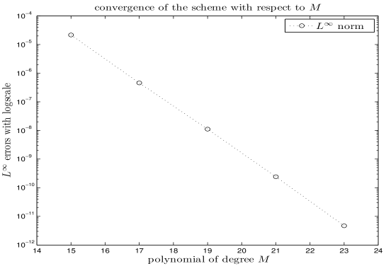
Figure 1. $L^{\infty}$-errors versus the degree of freedom for fine approximation $M$ with $\tilde{M}=13,N=20$.

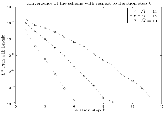
Figure 2. $L^{\infty}$-errors versus iteration numbers $k$ with ${M}=25,N=20$, $\tilde{M}=11,12,13$.

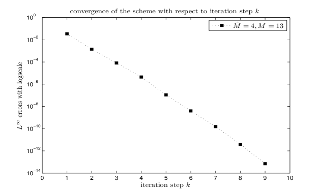
Figure 3. $L^{\infty}$-errors versus iteration number $k$ with $M=13,N=20,\tilde{M}=4$, and $T=20$.

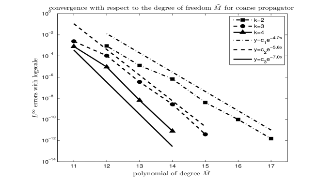
Figure 4. $L^{\infty}$-errors versus the degree of freedom in coarse approximation $\tilde{M}$ with ${M}=25$,$N=20$ and $k=2,3$, and 4.

Example 5.2.

Consider the Volterra integral equation with the kernel of exponential form $K(t,s)=(t-s)e^{s-t}$ and exact solution $u(t)=\frac{1}{4}(2t-1+e^{-2t})$.

We repeat the investigation of the convergence behavior of numerical solutions as in the first test. The $L^{\infty}$-errors of numerical solutions versus $M$ with $\tilde{M}=5,N=20$ are plotted in Figure 5. It is seen that the convergence remains exponential with respect to $M$ if the scheme is iterated a large enough step, and it appears that the growth in $t$ of the exact solution does not affect the convergence rate even for $T=100$.

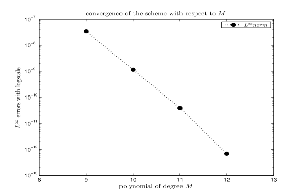
Figure 5. $L^{\infty}$-errors versus $M$ with $\tilde{M}=5,N=20$.

6. Parallelism Efficiency

Although not yet tested in a parallel machine, the parallelism efficiency of the proposed scheme can be investigated through a cost estimate. To simplify the cost estimation, we suppose that the inter-processor communication cost in the implementation of the parallel in time scheme is negligible as compared to the overall cost. The parallelism efficiency is demonstrated by a cost comparison between the parallel in time scheme (2.5)-(2.6) and the classical sequential scheme based on the corresponding fine mesh.

Firstly, the classical sequential scheme based on the fine mesh consists of solving the problems $\mathcal{F}_{n}\left(t,U_{1},U_{2},\cdots,U_{n-1}\right)$ consecutively for $n=1,\cdots,N$. The computational complexity is equal to the sum of all the elementary operations in $I_{n},n=1,\cdots,N$. Denote the total computational cost by $\mathcal{C}_{\mathcal{F}}$ and the cost for $n$-th subproblem by $\mathcal{C}^{n}_{\mathcal{F}}$. Then

$$\mathcal{C}_{\mathcal{F}}=\sum\limits_{n=1}^{N}\mathcal{C}^{n}_{\mathcal{F}}.$$

Neglecting the cost of evaluating the integral terms on the right hand sides, the spectral discretization $\mathcal{F}_{n}$ produces an elementary cost $\mathcal{C}^{n}_{\mathcal{F}}$ approximately equal to $\mathcal{O}(M^{2}M)$, where $\mathcal{O}(M^{2})$ is the number of operations needed for the matrix vector multiplication and $\mathcal{O}(M)$ is the estimated iteration number required to achieve the convergence of the iterative method. As a result, the total computational complexity of the sequential fine solutions is

(6.5) $$\mathcal{C}_{\mathcal{F}}=\mathcal{O}(NM^{3}).$$

If we implement the scheme (2.5)-(2.6) in a parallel architecture with enough processors, then the total computational time corresponds to the cost to solve a sequential set of $N$ coarse subproblems and a fine subproblem in a single processor. The cost of solving the sequential set of $N$ coarse subproblems is estimated to be $\sum^{N}_{n=1}\mathcal{C}^{n}_{\mathcal{G}}$, where $\mathcal{C}^{n}_{\mathcal{G}}=\mathcal{O}(\tilde{M}^{2}+M\tilde{M})$ is the cost to solve the $n$-th coarse subproblem, with $M\tilde{M}$ being the cost of the fine-to-coarse interpolation. Note that here we only count the number of operations needed for the matrix vector multiplication in the coarse mesh, which is equal to $\mathcal{O}(\tilde{M}^{2})$, because the Gauss-Seidel iterative method has been employed to solve the final linear system with the previous solution as the initial guess, and it is found that the convergence was achieved within a few iterations. For a same reason, the cost of solving a single fine subproblem is approximately $\mathcal{O}(M^{2})$. Note also, in the implementation of the parallel in time scheme there is a need to interpolate the solution between the fine mesh and coarse mesh, the cost of which is $\mathcal{O}(NM\tilde{M})$. Therefore if $K$ is the number of iterations required to achieve the desired convergence of the parallel in time algorithm, then the total computational complexity is

(6.6) $$K\Big{[}\mathcal{O}(N\tilde{M}^{2}+NM\tilde{M})+\mathcal{O}(M^{2})+\mathcal{O}(NM\tilde{M})\Big{]}.$$

Comparing (6.5) with (6.6), we obtain a speed up (i.e., the percentage with respect the sequential scheme) close to

$$\mathcal{O}\left(K\frac{\tilde{M}^{2}}{M^{3}}+K\frac{\tilde{M}}{M^{2}}+\frac{K}{NM}\right)^{-1}.$$

It can be verified that in general case the speed up is better than $\mathcal{O}(M/K)$. In some particular cases, for example if the number of degrees of freedom for the coarse solver is far less than that of the fine solver, i.e., $\tilde{M}\ll M$ or $\tilde{M}N=M$, then the speed up by using the parallel in time algorithm would be close to $\mathcal{O}(\frac{NM}{K})$.

References

- [1] G. Bal. Parallelization in time of (stochastic) ordinary differential equations. Math. Meth. Anal. Num., 2003.
- [2] G. Bal and Y. Maday. A parareal time discretization for non-linear PDEs with application to the pricing of an American put. in Proceedings of the Workshop on Domain Decomposition, LNCSE Series, 23:189–201, 2001.
- [3] H. Brunner. Collocation methods for Volterra integral and related functional differential equations. Cambridge Univ Press, 2004.
- [4] C. Canuto, M.Y. Hussaini, A. Quarteroni, and T.A. Zang. Spectral methods: Fundamentals in single domains. Springer, Berlin, 2006.
- [5] Y. Chen and T. Tang. Convergence analysis of the Jacobi spectral-collocation methods for Volterra integral equations with a weakly singular kernel. Mathematics of computation, 79(269):147–167, 2010.
- [6] N. Debit, M. Garbey, R. Hoppe, D. Keyes, Y. Kuznetsov, and J. Periaux. Domain decomposition methods in science and engineering. Internat. Center for Numerical Methods in Engineering, CIMNE, 2002.
- [7] C. Farhat and M. Chandesris. Time-decomposed parallel time-integrators: theory and feasibility studies for fluid, structure, and fluid-structure applications. International Journal for Numerical Methods in Engineering, 58(9):1397–1434, 2003.
- [8] P. Fischer, F. Hecht, and Y. Maday. A parareal in time semi-implicit approximation of the Navier-Stokes equations. in Proceedings of the 15th International Domain Decom- position Conference, Lect. Notes Comput. Sci. Eng. 40, R. Kornhuber, R. H. W. Hoppe, J. Péeriaux, O. Pironneau, O. B. Widlund, and J. Xu, eds., pages 433–440, 2003.
- [9] M.J. Gander and S. Vandewalle. Analysis of the parareal time-parallel time-integration method. ANALYSIS, 29(2):556–578, 2007.
- [10] S. Larsson, V. Thomee, and L. B. Wahlbin. Numerical solution of parabolic integro-differential equations by the discontinuous Galerkin method. Math. Comput., 67:45–71, 1998.
- [11] X. Li and C. Xu. A Space-Time Spectral Method for the Time Fractional Diffusion Equation. SIAM Journal on Numerical Analysis, 47(3):2108–2131, 2009.
- [12] X. Li and C. Xu. Existence and Uniqueness of the Weak Solution of the Space-Time Fractional Diffusion Equation and a Spectral Method Approximation. Commun. Comput. Phys., 8(5):1016–1051, 2011.
- [13] X.-J. Li and T. Tang. Convergence analysis of Jacobi spectral collocation methods for Abel-Volterra integral equations of second kind. Front. Math. China, 7:69–84, 2012.
- [14] J.L. Lions, Y. Maday, and G. Turinici. Résolution d’EDP par un schéma en temps pararéel. Comptes Rendus de l’Académie des Sciences-Series I-Mathematics, 332(7):661–668, 2001.
- [15] Y. Maday and G. Turinici. Parallel in time algorithms for quantum control: Parareal time discretization scheme. International Journal of Quantum Chemistry, 93(3):223–228, 2003.
- [16] G. Mastroianni and D. Occorsio. Optimal systems of nodes for Lagrange interpolation on bounded intervals. A survey. Journal of computational and applied mathematics, 134(1-2):325–341, 2001.
- [17] K. Mustapha, H. Brunner, H. Mustapha, and D. Schotazu. An -version discontinuous Galerkin method for integro-differential equations of parabolic type. SIAM J. Numer. Anal., 49:1369–1396, 2011.
- [18] J. Shen, T. Tang, and L.-L. Wang. Spectral Methods: Algorithms, Analysis and Applications. Springer, 2011. (Springer Series in Computational Mathematics).
- [19] T. Tang, X. Xu, and J. Cheng. On spectral methods for Volterra integral equations and the convergence analysis. J. Comput. Math, 26:825–837, 2008.
- [20] Z.-Q. Xie, X.-J. Li, and T. Tang. Convergence analysis of spectral Galerkin methods for Volterra type integral equations. J. Sci. Comput., Accepted, 2012.