A Number-Conserving Theory for Nuclear Pairing

Abstract

A microscopic theory for nuclear pairing is proposed through the generalized density matrix formalism. The analytical equations are as simple as that of the BCS theory, and could be solved within a similar computer time. The current theory conserves the exact particle number, and is valid at arbitrary pairing strength (including those below the BCS critical strength). These are the two main advantages over the conventional BCS theory. The theory is also of interests to other mesoscopic systems.

I Introduction

The BCS theory is first proposed as a microscopic theory for superconductivity BCS . Later it is adopted in nuclear physics for treating pairing correlations BCS_nucl1 ; BCS_nucl2 . After fifty years, it is still the “standard” treatment (see Ref. BCS_book ), mainly because of its simplicity and the convenience in adding higher-order correlations (for example by QRPA). However, there are two main disadvantages of the theory applied to the finite nucleus, as compared to macroscopic quantum systems. Firstly, by introducing quasi-particles, it destroys particle number conservation. Quite often, the fluctuation in particle number was not small relative to its average value. Secondly, for the nuclear system with finite level spacing, the BCS theory requires a minimal pairing strength. Below that strength it gives only trivial (vanishing) solutions, while in reality the pairing always has an effect.

The current treatment by the generalized density matrix (GDM) method does not have the above two deficiencies. Yet it is simple enough for further treatment of higher-order correlations within the same GDM framework. We will first present the formalism in Sec. II. Next the theory is applied to calcium isotopes in Sec. III with comparisons to the exact shell-model results and that of BCS. At last Sec. IV summarizes the work and discusses further directions.

II Formalism

The GDM formalism was originally introduced in Refs. kerman63 ; BZ ; Zele_ptps ; shtokman75 and recently reconsidered in Refs. Jia_1 ; Jia_2 ; Jia_3 . Until now its treatment of nuclear pairing correlations is limited to the conventional BCS, thus has the above discussed disadvantages. Here we explore the possibility of using the “pair condensate” (1) (with definite particle number) as the “variational” ground state, instead of the BCS “quasi-particle vacuum”. Below we set up the GDM formalism in a general way, but solve in this work only the lowest-order (mean-field) equations.

We assume that the ground state of the $2N$-particle system is a $N$-pair condensate,

$$|\phi_{N}\rangle=\frac{1}{\sqrt{\chi_{N}}}(P^{\dagger})^{N}|0\rangle,$$ (1)

where $\chi_{N}$ is a normalization factor that will be specified later [see Eq. (22)], and $P^{\dagger}$ is the pair creation operator

$$P^{\dagger}=\frac{1}{2}\sum_{1}v_{1}a_{1}^{\dagger}a_{\tilde{1}}^{\dagger}.$$ (2)

In Eq. (2) the summation runs over the entire single-particle space. The pair structure $v_{1}$ are parameters to be determined by the theory.

With the antisymmetrized fermionic Hamiltonian

$$H=\sum_{12}\epsilon_{12}a_{1}^{\dagger}a_{2}+\frac{1}{4}\sum_{1234}V_{1234}a_{1}^{\dagger}a_{2}^{\dagger}a_{3}a_{4},$$ (3)

we calculate the equations of motion for the one-body density matrix operators, $R_{12}\equiv a_{2}^{\dagger}a_{1}$ and $K_{12}=a_{2}a_{1}$,

$$[R_{12},H]=[f\{R\},R]_{12}-(K\Delta^{\dagger}\{K\})_{12}+(\Delta\{K\}K^{\dagger})_{12},$$ (4)

$${[}K_{12},H]=\Delta\{K\}_{12}+(Kf^{T}\{R\})_{12}+(f\{R\}K)_{12}$$

$$-(\Delta\{K\}R^{T})_{12}-(R\Delta\{K\})_{12},$$ (5)

where the self-consistent fields are defined as

$$W\{R\}_{12}=\sum_{34}V_{1432}R_{34},~{}~{}~{}f\{R\}=\epsilon+W\{R\},$$ (6)

$$\Delta\{K\}_{12}=\frac{1}{2}\sum_{34}V_{1234}K_{43}.$$ (7)

On the right-hand side of Eqs. (4) and (5) we have used the factorization

$$a_{4}^{\dagger}a_{3}^{\dagger}a_{2}a_{1}\circeq a_{4}^{\dagger}a_{1}\cdot a_{3}^{\dagger}a_{2}-a_{4}^{\dagger}a_{2}\cdot a_{3}^{\dagger}a_{1}+a_{4}^{\dagger}a_{3}^{\dagger}\cdot a_{2}a_{1},$$ (8)

$$a_{4}^{\dagger}a_{3}a_{2}a_{1}\circeq a_{4}^{\dagger}a_{1}\cdot a_{3}a_{2}-a_{4}^{\dagger}a_{2}\cdot a_{3}a_{1}+a_{4}^{\dagger}a_{3}\cdot a_{2}a_{1},$$ (9)

generalizing Eq. (11) in Ref. Jia_2 . In the presence of the pair condensate terms like $a_{4}^{\dagger}a_{3}^{\dagger}\cdot a_{2}a_{1}$ are not small. As before “$\circeq$” is used when an equation holds in the collective subspace but not in the full many-body space.

The method assumes that the Hamiltonian and the density matrix operators can be expanded as Taylor series of the bosonic mode operators (collective coordinate $\alpha$ and momentum $\pi$) within the collective subspace,

$$H\circeq\sum_{ml}\Lambda^{(m,2l)}\frac{1}{2}\frac{\{\alpha^{m},\pi^{2l}\}}{m!(2l)!},$$ (10)

and

$$R_{12}=a_{2}^{\dagger}a_{1}\circeq\sum_{mn}r^{(mn)}_{12}\frac{1}{2}\frac{\{\alpha^{m},\pi^{n}\}}{m!n!},$$ (11)

$$K_{12}=a_{2}a_{1}\circeq\sum_{mn}k^{(mn)}_{12}\frac{1}{2}\frac{\{\alpha^{m},\pi^{n}\}}{m!n!}.$$ (12)

In Eq. (12) $K_{12}$ destroys two particles, hence it connects the collective subspace with $2N$ particles to that with $2N-2$ particles. The first term $k^{(00)}\equiv\kappa$ is the usual “pair transition amplitude” between the ground states of neighboring even-even nuclei. Higher-order terms $k^{(mn)}$ represent the transition amplitudes between the collectively excited states (with phonons). Strictly speaking, the generalized density matrices ($r_{N,12}$, $k_{N,12}$), the mode operators ($\alpha_{N}$, $\pi_{N}$), and the bosonic Hamiltonian parameters $\Lambda^{(m,2l)}$ should have the label of particle number $2N$, and the GDM equations should be solved simultaneously for all the nuclei between two magic numbers, in a way similar to that in Ref. Zele_pairing . However in this work we will drop the label $N$, assuming neighboring even-even nuclei have similar collective modes ($\alpha_{N}\approx\alpha_{N-1}$, $\pi_{N}\approx\pi_{N-1}$) and density matrices ($r_{N}\approx r_{N-1}$, $k_{N}\approx k_{N-1}$). More careful treatment with explicit label $N$ will be discussed in the future.

Substituting the expansions (10), (11) and (12) into the equations of motion (4) and (5), calculating commutators of bosonic operators $\alpha$ and $\pi$, we arrive at the GDM set of equations. In this work we consider only the lowest-order (mean-field) equations:

$$0=[f,\rho]-\kappa\delta^{\dagger}+\delta\kappa^{\dagger},$$ (13)

$$(\Lambda^{(00)}_{N}-\Lambda^{(00)}_{N-1})\kappa=f\kappa+\delta-\delta\rho^{T}-\rho\delta+\kappa f^{T},$$ (14)

where $\rho\equiv r^{(00)}$, $\kappa\equiv k^{(00)}$, $f=\epsilon+W\{\rho\}$, and $\delta=\Delta\{\kappa\}$ are leading terms in the expansions of respective quantities (6,7,11,12). $\Lambda^{(00)}_{N}$, the leading term in the bosonic Hamiltonian (10), is the binding energy of the $N$-pair condensate (1). Usually the difference $\Lambda^{(00)}_{N}-\Lambda^{(00)}_{N-1}$ is not small and should be kept.

On the ground state (1), $\rho$ and $\kappa$ are “diagonal”:

$$\rho_{12}=\langle\phi_{N}|a_{2}^{\dagger}a_{1}|\phi_{N}\rangle=\delta_{12}n_{1},$$ (15)

$$\kappa_{12}=\langle\phi_{N-1}|a_{2}a_{1}|\phi_{N}\rangle=\delta_{\tilde{1}2}s_{1},$$ (16)

where $s_{1}$ and $n_{1}$ are functions of the pair structure $v$ (2), given later by the recursive formula (23). In a realistic shell-model calculation, usually each single-particle level has distinct spin and parity, thus both $f$ and $\delta$ are “diagonal”:

$$f_{12}=\delta_{12}e_{1},$$ (17)

$$\delta_{12}=\delta_{1\tilde{2}}g_{1}.$$ (18)

Under Eqs. (15,16,17,18), Eq. (13) is satisfied automatically, and Eq. (14) becomes

$$\Lambda^{(00)}_{N}-\Lambda^{(00)}_{N-1}=2e_{1}+g_{1}\frac{2n_{1}-1}{s_{1}}.$$ (19)

Equation (19) is the main equation of the theory. It implies that the right-hand side is independent of the single-particle label $1$, which gives $\Omega-1$ constraints for a single-particle space of dimension $2\Omega$ ($\Omega$ time-reversal pairs). These constraints fix the $\Omega-1$ parameters in Eq. (2) (a common factor in $v_{1}$ does not matter), which completes the theory. Notice that Eq. (19) has non-trivial (“non-zero”) solution at infinitesimal pairing (infinitesimal $g_{1}$).

At last we supply the formula for the recursive calculation of $\rho$ (15) and $\kappa$ (16) in terms of $v$ (2). Introducing $P_{1}^{\dagger}=a_{1}^{\dagger}a_{\tilde{1}}^{\dagger}$ and

$$t^{1}_{N}=\langle 0|P^{N-1}P_{1}(P^{\dagger})^{N}|0\rangle,$$ (20)

it is easy to deduce the recursive formula

$$t^{1}_{N}=\frac{1}{2}N\cdot v_{1}\sum_{2}v_{2}t^{2}_{N-1}-N(N-1)\cdot(v_{1})^{2}t^{1}_{N-1},$$ (21)

with initial value $t^{1}_{N=1}=v_{1}$. Then the normalization factor $\chi_{N}$ in Eq. (1) is expressed in terms of $t_{N}$ as

$$\chi_{N}=\frac{1}{2}\sum_{1}v_{1}t^{1}_{N}.$$ (22)

$t_{N}^{1}$ and $\chi_{N}$ are polynomials of $v$. Finally the expressions for $n_{1}$ (15) and $s_{1}$ (16) are

$$n_{1}=\frac{Nv_{1}t^{1}_{N}}{\chi_{N}},~{}~{}~{}s_{1}=\frac{t^{1}_{N}}{\sqrt{\chi_{N}\chi_{N-1}}}.$$ (23)

The functional forms of $n$ and $s$ in terms of $v$ (2) are “kinematics” of the system (like the “kinematic” Clebsch-Gordan coefficients for rotational symmetry), which can be calculated (and stored or tabulated) once for all for a given model space. The main computing-time cost of the method should be that to solve Eq. (19). In fact, Eq. (19) is a better behaved equation compared to the BCS equation. It involves essentially ratio of two polynomials but no square roots.

As a simple check we consider the degenerate pairing model. Equations (21) and (22) become $t_{N}=Nv^{2}(\Omega-N+1)t_{N-1}$ and $\chi_{N}=\Omega vt_{N}$, which in turn gives $n=N/\Omega$ and $s=\sqrt{N(\Omega-N+1)}/\Omega$ according to Eq. (23). They agree with the known results. The right-hand side of Eq. (19) becomes $2\epsilon+(G\Omega s)(\frac{2N/\Omega-1}{s})=2\epsilon+G(2N-\Omega)$, which is the correct binding energy difference $\Lambda^{(00)}_{N}-\Lambda^{(00)}_{N-1}$.

III Realistic Applications

We apply the theory to calcium isotopes, using the well established FPD6 interaction fpd6 , where ⁴⁰Ca is taken as an inertia core, and the valence neutrons are distributed in $4$ single-neutron levels $0f_{7/2}$, $1p_{3/2}$, $0f_{5/2}$, and $1p_{1/2}$.

We first consider the nucleus ⁴⁸Ca, where the BCS results in only a trivial zero solution due to the “complete filling” of the $0f_{7/2}$ orbit. In the Hamiltonian (3), we keep only the pairing matrix elements $\langle jj;0|V|j^{\prime}j^{\prime};0\rangle$ of FPD6 for the two-body interaction $V$, and the single-particle energies $\epsilon$ are fixed by experimental data as following. From the spectrum of ⁴⁹Ca we read $\epsilon_{p_{1/2}}-\epsilon_{p_{3/2}}=2.023$MeV, $\epsilon_{f_{5/2}}-\epsilon_{p_{3/2}}=3.585$MeV. And the neutron absorption energy of ⁴⁸Ca gives $\epsilon_{p_{3/2}}=-5.146$MeV. $\epsilon_{f_{7/2}}$ is estimated within the single-$j$ degenerate pairing model as $\epsilon_{f_{7/2}}=-9.945{\rm MeV}+0.541{\rm MeV}=-9.404{\rm MeV}$, where $-9.945$MeV is the neutron emission energy of ⁴⁸Ca and $0.541$MeV is the FPD6 pairing strength for the $0f_{7/2}$ orbit.

The results are given in Fig. 1. The realistic case corresponds to $G=1$ in the horizontal axis. We see that the GDM calculation reproduces quite well the exact results (by the shell-model code NuShellX MSU_Nu ) of occupation numbers $n_{J}$ and pair emission amplitudes $s_{J}$, while BCS fails giving only trivial zero results. To see how the theory behaves at different pairing strength, an artificial factor $G$ is introduced that is multiplied onto the FPD6 pairing two-body matrix elements. We do a set of calculations at different values of $G$ (from $0.2$ to $2.0$). The GDM theory does quite well at all pairing strength, including those below the critical value ($G_{c}=1.345$) of BCS. It even gets one detail right: the inversion (around $G=1.6$) of relative positions of the two very close curves for $f_{5/2}$ and $p_{1/2}$. Because some numbers in Fig. 1 are very close and difficult to see, we also list them in Table 1.

Next we test the theory in different nuclei. The chain of calcium isotopes is calculated with mass number $42\leq A\leq 58$. For simplicity in this example we fix the single-particle energies $\epsilon$ by the FPD6 ones: $\epsilon_{f_{7/2}}=-8.3876$MeV, $\epsilon_{p_{3/2}}=-6.4952$MeV, $\epsilon_{f_{5/2}}=-1.8966$MeV, and $\epsilon_{p_{1/2}}=-4.4783$MeV. And in the two-body interaction $V$ we still keep only the FPD6 pairing matrix elements. The results are shown in Fig. 2. The GDM method reproduce the exact results quite well, even the sudden changes around $A=54$.

IV Summary

In summary, we explored the possibility of using the pair condensate (1) instead of the quasi-particle vacuum as the starting point of the GDM method. As the lowest order result, a theory for nuclear pairing is proposed that conserves the exact particle number and is valid at arbitrary pairing strength (including those below the critical point of BCS). Correlations beyond the mean field could be studied solving higher-order equations in the GDM formalism.

Odd-mass nuclei could be calculated consistently. The effective Hamiltonian, $\langle 2N+1|H|2N+1\rangle=\langle 2N|aHa^{\dagger}|2N\rangle$, was calculated by substituting Eq. (3) into the above expression and then using factorizations similar to Eq. (8), where the density matrices $a^{\dagger}a$ and $aa$ are known from the neighboring even-even nuclei. Spectroscopic factors, $\langle 2N-1|a|2N\rangle=\langle 2N|a^{\dagger}a|2N\rangle$, could also be calculated in a similar way. These will be studied in the future.

The author gratefully acknowledges discussions with Prof. Vladimir Zelevinsky.

a

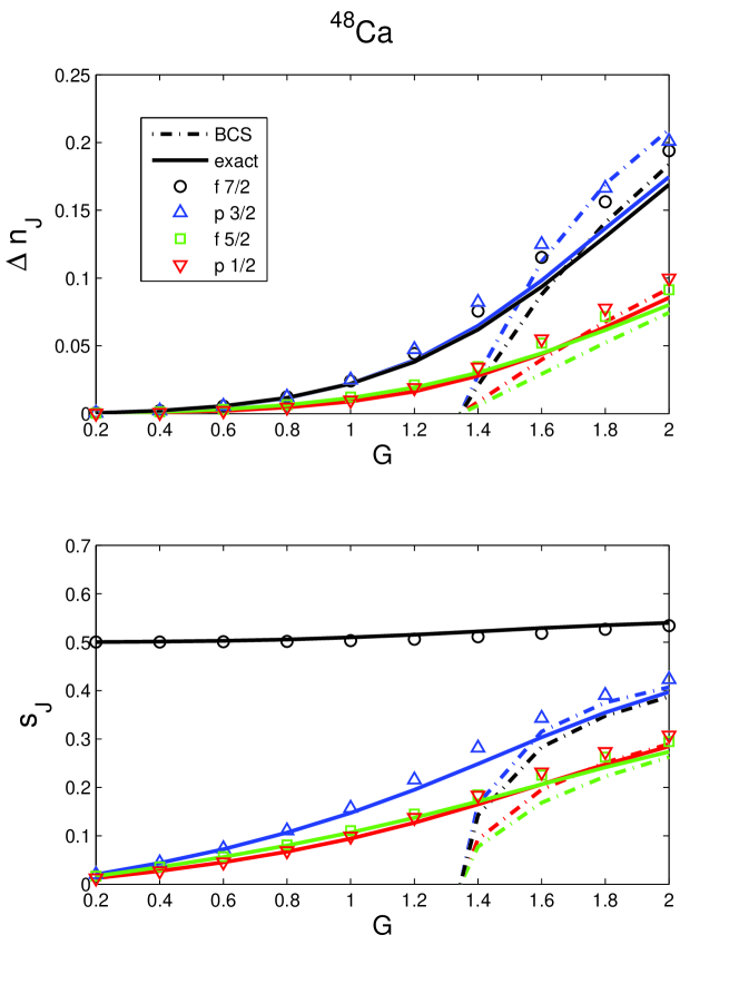
Figure 1: (Color online) Occupation numbers $n_{J}$ (15) and pair emission amplitudes $s_{J}$ (16) in ⁴⁸Ca as a function of pairing strength $G$. In the calculation the FPD6 pairing two-body matrix elements are multiplied by $G$ ($G=1$ is realistic). The upper panel plots $\Delta n_{J}$, the derivations from the naive Fermi occupation ($\Delta n_{J}=1-n_{f7/2},n_{p3/2},n_{f5/2},n_{p1/2}$). The solid lines and dashed-dotted lines show the exact results (by NuShellX) and BCS results respectively. The symbols show the GDM results, where black circles, blue up-triangles, green squares, and red down-triangles are for single-particle levels $f_{7/2}$, $p_{3/2}$, $f_{5/2}$, and $p_{1/2}$, respectively. The same color convention is used in plotting the solid lines (exact) and dashed-dotted lines (BCS). The plotted BCS $s_{J}$ is defined as $s_{1}=~{}_{\rm{BCS}}\langle{\phi_{N}}|a_{\tilde{1}}a_{1}|{\phi_{N}}\rangle_{\rm{BCS}}=\sqrt{n_{1}(1-n_{1})}$.

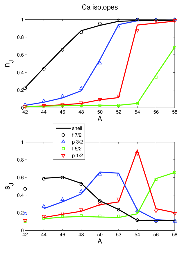
Figure 2: (Color online) Occupation numbers $n_{J}$ (15) and pair emission amplitudes $s_{J}$ (16) in calcium isotopes ($A$ is the mass number). The solid lines show the shell-model results (by NuShellX), using the FPD6 single-particle energies and pairing two-body matrix elements. The symbols show the GDM results, where black circles, blue up-triangles, green squares, and red down-triangles are for single-particle levels $f_{7/2}$, $p_{3/2}$, $f_{5/2}$, and $p_{1/2}$, respectively. The same color convention is used in plotting the solid lines (shell).

Table 1: Results of the shell-model and GDM calculations plotted in Fig. 1. $n_{J}$ are occupation numbers, and $s_{J}$ are pair emission amplitudes.

$G=$	$0.2$	$0.4$	$0.6$	$0.8$	$1.0$	$1.2$	$1.4$	$1.6$	$1.8$	$2.0$
$n_{f_{7/2}}~{}{\rm{exact}}$	0.9996	0.9979	0.9945	0.9883	0.9780	0.9618	0.9381	0.9065	0.8695	0.8311
GDM	0.9995	0.9979	0.9944	0.9877	0.9759	0.9557	0.9244	0.8848	0.8438	0.8061
$n_{p_{3/2}}~{}{\rm{exact}}$	0.0004	0.0019	0.0053	0.0115	0.0222	0.0394	0.0648	0.0983	0.1366	0.1747
GDM	0.0004	0.0020	0.0054	0.0122	0.0249	0.0474	0.0822	0.1249	0.1663	0.2010
$n_{f_{5/2}}~{}{\rm{exact}}$	0.0003	0.0013	0.0032	0.0064	0.0116	0.0192	0.0302	0.0445	0.0616	0.0802
GDM	0.0003	0.0013	0.0032	0.0066	0.0122	0.0212	0.0346	0.0520	0.0716	0.0913
$n_{p_{1/2}}~{}{\rm{exact}}$	0.0001	0.0008	0.0021	0.0045	0.0089	0.0163	0.0278	0.0439	0.0638	0.0856
GDM	0.0002	0.0007	0.0021	0.0047	0.0098	0.0190	0.0342	0.0549	0.0777	0.0999
$s_{f_{7/2}}~{}{\rm{exact}}$	0.5002	0.5010	0.5026	0.5054	0.5097	0.5153	0.5221	0.5291	0.5350	0.5398
GDM	0.5001	0.5003	0.5007	0.5016	0.5032	0.5061	0.5112	0.5183	0.5264	0.5340
$s_{p_{3/2}}~{}{\rm{exact}}$	0.0201	0.0438	0.0723	0.1064	0.1472	0.1951	0.2485	0.3035	0.3544	0.3969
GDM	0.0201	0.0441	0.0735	0.1103	0.1571	0.2155	0.2815	0.3430	0.3902	0.4231
$s_{f_{5/2}}~{}{\rm{exact}}$	0.0167	0.0353	0.0562	0.0798	0.1067	0.1372	0.1709	0.2064	0.2413	0.2734
GDM	0.0167	0.0354	0.0566	0.0812	0.1103	0.1449	0.1845	0.2253	0.2627	0.2948
$s_{p_{1/2}}~{}{\rm{exact}}$	0.0123	0.0270	0.0450	0.0670	0.0940	0.1268	0.1649	0.2061	0.2473	0.2848
GDM	0.0123	0.0272	0.0455	0.0688	0.0988	0.1373	0.1836	0.2313	0.2734	0.3076

References

- (1) J. Bardeen, L. N. Cooper, and J. R. Schrieffer, Phys. Rev. 106, 162 (1957); Phys. Rev. 108, 1175 (1957).
- (2) A. Bohr, B. R. Mottelson, and D. Pines, Phys. Rev. 110, 936 (1958).
- (3) S. T. Belyaev, K. Dan. Vidensk. Selsk. Mat. Fys. Medd. 31, (11) (1959).
- (4) Ricardo A Broglia, and Vladimir Zelevinsky, Fifty Years of Nuclear BCS: Pairing in Finite Systems (World Scientific, 2013).
- (5) A. Kerman and A. Klein, Phys. Rev. 132, 1326 (1963).
- (6) S.T. Belyaev and V.G. Zelevinsky, Yad. Fiz. 11, 741 (1970) [Sov. J. Nucl. Phys. 11, 416 (1970)]; Yad. Fiz. 16, 1195 (1972) [Sov. J. Nucl. Phys. 16, 657 (1973)]; Yad. Fiz. 17, 525 (1973) [Sov. J. Nucl. Phys. 17, 269 (1973)].
- (7) V.G. Zelevinsky, Prog. Theor. Phys. Suppl. 74-75, 251 (1983).
- (8) M.I. Shtokman, Yad. Fiz. 22, 479 (1975) [Sov. J. Nucl. Phys. 22, 247 (1976)].
- (9) L. Y. Jia, Phys. Rev. C 84, 024318 (2011).
- (10) L. Y. Jia, and V. G. Zelevinsky , Phys. Rev. C 84, 064311 (2011).
- (11) L. Y. Jia, and V. G. Zelevinsky , Phys. Rev. C 86, 014315 (2012).
- (12) Alexander Volya, and Vladimir Zelevinsky, nucl-th/9912068; MSUCL-1144 (1999).
- (13) W.A. Richter, M.G. Van Der Merwe, R.E. Julies, and B.A. Brown, Nucl. Phys. A523, 325 (1991).
-
(14)
NuShellX@MSU, B. A. Brown and W. D. M. Rae,
http://www.nscl.msu.edu/ brown/resources/resources.html