The Dual Frequency Anisotropic Magneto-Optical Trap

Abstract

The cloud of cold atoms produced by a Magneto-Optical Trap is known to exhibit instabilities. We examine in this paper in which limits it could be possible to realize an experimental trap similar to the configurations studied theoretically, i.e. mainly traps where one direction is privileged. We study the static behavior of an anisotropic trap, where anisotropy results essentially from the use of two different laser frequencies for the arms of the trap. Such a trap has very surprising behaviors, in particular the cloud disappears for some laser frequencies, while it exists for smaller and larger frequencies. A model is build to explain these behaviors. We show in particular that, to reproduce the experimental observations, the model has to take into account the cross saturation effects. Moreover, the couplings between the different directions cannot be neglected.

1 Introduction

The spectacular results obtained during the last decades in the domain of the experimental quantum physics required all as a first step to cool atoms with a Magneto-Optical Trap (MOT). The cold atoms produced in such a MOT can then be put in lattices lattices , used to produce cold molecules molecules or be further cooled down to produce Bose-Einstein condensates BEC . But the MOT itself is also an interesting object. Many questions remain unanswered, and the usual theoretical descriptions are hardly enough to describe the stationary behavior of the cloud of cold atoms produced by a MOT. But in many situations, this cloud exhibits spatio-temporal instabilities wilkowski2000 ; labeyrie2006 , for which the development of new models is necessary. And indeed, several models were recently proposed wilkowski2000 ; labeyrie2006 ; hennequin2004 ; distefano2003 ; distefano2004 ; pohl2006 ; mendonca2008 ; romain2011 . The search for a model describing correctly the dynamics of cold atoms in a MOT is primarily motivated by the hope to understand the mechanisms leading to such a complex behavior. But it regained recently interest when it was shown that this system is formally very close to some plasmas. In particular, it was demonstrated that the cloud of cold atoms is described by a Vlasov-Fokker-Planck equation, and the analogies with plasmas were extensively discussed romain2011 .

Unfortunately, none of these models lead to a satisfactory description of the experimental observations. For most of them, the theoretical predictions differ deeply from the experimental observations labeyrie2006 ; pohl2006 ; mendonca2008 . Some models give a good qualitative description of the observed dynamics wilkowski2000 ; hennequin2004 . But they modelize a 1D MOT, and direct quantitative comparison with experiments is not possible, as all experimental observations of the MOT dynamics concern 3D MOTs. Thus, to go further, it is necessary either to generalize these models in 3D, or to realize 1D experiments.

A 1D MOT in this context is more precisely a MOT where atoms are trapped in 3D, but where instabilities occur only along one direction of space, called in the following the unstable direction. Such a MOT is an anisotropic MOT rather than a 1D MOT. It could be obtained if the unstable direction of space is not coupled to the other directions. Unfortunately, the effective coupling between the different arms of a MOT has been poorly studied, while several mechanisms are known to possibly induced such a coupling. For instance, the well known multiple scattering has never been studied from this point of view. The cross saturation effects are also a possible coupling mechanism, which is usually neglected. It is important to evaluate precisely these couplings, as, if they cannot be neglected, other solutions have to be used to force the system to be stationary in two directions of space.

Various anisotropic traps have been studied in the past. The interesting configurations for our purposes are those where the anisotropy is introduced on a parameter controlling the instabilities of the MOT. In distefano2003 ; distefano2004 , it is shown that at least two control parameters allow to tune the trap from a stationary situation to an unstable dynamics: the intensity of the laser trapping beams, and the detuning between the laser trapping beam frequency and that of the atomic transition used to cool the atoms. The main difference between these two control parameters concerns the range on which occurs the transition from a stable behavior to instabilities. The results in distefano2004 show that for intensity, this range spreads over almost one order of magnitude, whereas for the detuning, it is less than a factor 2.

Traps with anisotropic laser beam intensities or magnetic field gradients have already been studied stites2004 ; vengalattore2003 . One of the main results is that for clouds with a large aspect ratio, multiple scattering disappears vengalattore2003 . This puts in evidence the coupling between the different directions of space through the multiple scattering, and this means that the anisotropy should be as small as possible to limit the effect of this coupling. Thus in our case, introducing the anisotropy through the frequency detuning should be a better solution, but to our knowledge, this type of anisotropic trap has not yet been studied.

We present in this paper results about a dual frequency trap with different frequency detunings along the different axes. Experimental measurements show that such a trap has very unusual behaviors, in particular the disappearance of the atomic cloud for some detuning pairs, while cold atoms are obtained on both sides of these frequencies. We show that the usual models, which neglect the cross saturation effects, are not able to reproduce these experimental observations. We build another model which takes into account the cross saturation effects, and show that the behaviors predicted by this model are qualitatively consistent with the experimental observations.

2 Experimental results

2.1 Experimental setup

We work with a Cesium-atom MOT in the usual $\sigma^{+}-\sigma^{-}$ configuration. Each of the three arms of the trap is formed by counter-propagating beams resulting from the reflection of the three forward beams, obtained from the same laser diode. Beams propagate following three perpendicular directions, one of them being the axis of the coils producing the magnetic field. In this so-called parallel direction, the forward beam is characterized by the intensity $I_{\parallel}$ and the detuning $\Delta_{\parallel}=\omega_{\parallel}-\omega_{0}$, where $\omega_{\parallel}$ is the beam frequency and $\omega_{0}$ the atomic frequency. In the two other directions, the beams are characterized by the intensity $I_{\perp}$ and the detuning $\Delta_{\perp}=\omega_{\perp}-\omega_{0}$. When $I_{\parallel}=I_{\perp}$ and $\Delta_{\parallel}=\Delta_{\perp}$, we have the most common MOT. However, this usual MOT is already not isotropic, although it is often considered as so. Indeed, the magnetic field is produced by a pair of coils in an anti-Helmholtz configuration. Thus the magnetic field gradient along the parallel direction is twice that in the perpendicular directions, leading to a fixed anisotropy on the restoring force of the trap. We can characterize such a trap as a balanced single-frequency trap. As discussed above, we will focus here on the effects induced by a frequency anisotropy, i.e. a balanced or unbalanced dual-frequency trap ($\Delta_{\parallel}\neq\Delta_{\perp}$).

In the present study, we focus on the stationary cloud. This cloud can be characterized by its number of atoms and the spatial distribution of these atoms. To measure the number of atoms, we just need a photodiode to record the total fluorescence emitted by the atoms in the cloud. Fluorescence is proportional to the number $N$ of atoms in the cloud, and thus it is a good indicator of $N$. However, the proportionality coefficient depends on the laser intensities and detunings. For large saturations, this coefficient may be considered as constant, but in the other cases, it decreases as the detunings increase. In the experimental results presented here, taking into account this correction factor would lead to an increase of $N$ by a factor lower than 3 for large detunings. As this correction induces no qualitative change in the behaviors described here, we did not apply it on the curves shown below.

The distribution of atoms is usually measured through the radius of the cloud. However, we introduce now a new anisotropy in the trap, which is expected to lead to an ellipsoidal cloud. Thus a measurement of the cloud size in the two main directions appears necessary. This measurement is performed by using a camera. Recorded pictures are analyzed by a software which fits the atomic cloud on a 2D gaussian. The result of the fit gives us the semi-axes $L_{\parallel}$ and $L_{\perp}$ of the ellipsoid, but a convenient value to monitor is the ellipticity $\varepsilon=L_{\perp}/L_{\parallel}$, as we expect a correlation between $\varepsilon$ and the anisotropy.

2.2 Atomic cloud behavior

We have studied the evolution of the cloud as a function of the frequency difference $\Delta_{\parallel}-\Delta_{\perp}$, for different detunings and trap beam intensities, including cases where intensities following the two directions are different. A typical experimental measurement consists in recording the evolution of the number $N$ of atoms in the cloud and the cloud sizes as a function of $\Delta_{\parallel}$, the other parameters, in particular $\Delta_{\perp}$, $I_{\perp}$ and $I_{\parallel}$, being constant. The measurements are then repeated for different values of $\Delta_{\perp}$, $I_{\perp}$ and $I_{\parallel}$.

Figure 1: Number $N$ of atoms in the cloud versus $\Delta_{\parallel}$ for $\Delta_{\perp}=-2\Gamma$ and $I_{\parallel}\simeq I_{\perp}\simeq 2I_{S}$.

Fig. 1 shows the typical evolution of the fluorescence on the interval where it is measurable. In this example, $\Delta_{\perp}=-2\Gamma$, where $\Gamma=2\pi\times 5.234\,\mathrm{MHz}$ is the natural width of the transition, $-6.5\Gamma<\Delta_{\parallel}<0$ and $I_{\parallel}\simeq I_{\perp}\simeq 2I_{S}$ where $I_{S}=1.1\,\mathrm{mW/cm^{2}}$ is the saturation intensity. At the degeneracy $\Delta_{\parallel}=\Delta_{\perp}$, we have a standard balanced single-frequency MOT.

On each side of this degeneracy, at a typical frequency difference $\Delta_{\parallel}-\Delta_{\perp}=\pm 0.5\Gamma$, the number of atoms exhibits a gap. We did not study in details the mechanisms at the origin of this behavior, mainly because in the scope of the present work, it is more interesting to introduce a large difference between $\Delta_{\parallel}$ and $\Delta_{\perp}$, to obtain a large anisotropy. However, it can be noticed that the frequencies where the gaps occur, are of the same order of magnitude as the energy shifts between the ground state Zeeman sublevels grison1991 . Thus it is probable that this behavior originates in a Raman resonance between Zeeman sub-levels of the fundamental atomic level.

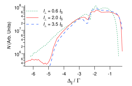
Figure 2: Number $N$ of atoms in the cloud versus $\Delta_{\parallel}$ for $\Delta_{\perp}=-2\Gamma$, $I_{\parallel}\simeq 2I_{S}$ and different values of $I_{\perp}$.

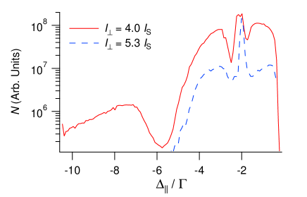
Figure 3: Number $N$ of atoms in the cloud versus $\Delta_{\parallel}$ for $\Delta_{\perp}=-2\Gamma$, $I_{\parallel}\simeq 9I_{S}$ and different values of $I_{\perp}$.

Except for these gaps, the number of atoms in the MOT decreases monotonically as $\left|\Delta_{\parallel}-\Delta_{\perp}\right|$ is increased. On the blue side, it vanishes when $\Delta_{\parallel}$ reaches the resonance, as expected when atoms are no more trapped in the parallel direction. On the red side, we observe different behaviors, depending on the laser intensities. More precisely, the observed behavior depends mainly on $I_{\perp}$, and thus we find similar evolutions in traps with $I_{\parallel}=I_{\perp}$ or $I_{\parallel}\neq I_{\perp}$. These behaviors are illustrated on Fig. 2, where the three curves show the evolution of the number of atoms on a log scale for three different values of $I_{\perp}$. $I_{\parallel}$ and $\Delta_{\perp}$ are as in Fig. 1. When $I_{\perp}\lesssim I_{S}$, the number of atoms decreases progressively until it vanishes for $\Delta_{\parallel}\simeq-7\Gamma$. When $I_{\perp}\gg I_{S}$, the decreasing is much faster, with a disappearance of the cloud at $\Delta_{\parallel}\simeq-5\Gamma$. For intermediate intensities, the curve is the same as that of Fig. 1: the decreasing of the number of atoms is also fast, and the cloud disappears at $\Delta_{\parallel}\simeq-5\Gamma$. But the curve exhibits a rebound, which means that the cloud re-appears until it definitively disappears at $\Delta_{\parallel}\simeq-7\Gamma$. The number of atoms in the rebound may be consequent: Fig. 3 shows the rebound obtained for $I_{\parallel}=9I_{S}$, $I_{\perp}=4I_{S}$ and $\Delta_{\perp}=-2\Gamma$. $N$ reaches in this case more than 1% of the main maximum, while $\Delta_{\parallel}=-8\Gamma$. Fig. 3 shows that in this situation again, when $I_{\perp}$ is increased, the rebound disappears and the cloud vanishes for a small detuning. In fact, the behavior shown on Fig. 2 appears to be general, whatever the values of $-2\leq\Delta_{\perp}\leq-1$ and $I_{S}\leq I_{\parallel}\leq 12I_{S}$. The only explanation of this type of behavior is that strong couplings between the different directions arise.

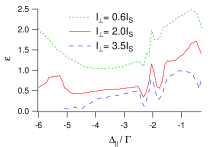
Figure 4: Ellipticity $\varepsilon$ of the atomic cloud versus $\Delta_{\parallel}$ for $\Delta_{\perp}=-2\Gamma$, $I_{\parallel}\simeq 2I_{S}$ and different values of $I_{\perp}$.

As expected, the cloud shape depends on the trap anisotropy. Fig. 4 shows the evolution of the ellipticity $\varepsilon$ for the same parameters as in Fig. 2. As for $N$, the curves exhibit around the single-frequency MOT $\Delta_{\parallel}=\Delta_{\perp}$ rapid variations which probably also originate in the Raman resonance discussed above. Except for that point, the ellipticity increases on the blue side of the isotropic trap, before it decreases rapidly when the resonance is closely approached. On the red side, the ellipticity decreases slowly, and then, depending on the value of $I_{\perp}$, it may increase again for larger detunings. We can also notice that when $I_{\perp}$ is increased, $\varepsilon$ globally decreases, as it could be naively expected: the larger transverse intensity compresses the cloud in the transverse direction.

In summary of these experimental observations, several non trivial behaviors occur in the anisotropic trap. Strong couplings between the different directions show up. We were not able to observe instabilities in this configuration, and we attribute it to these couplings. The most intriguing behavior is the disappearance and re-appearance of the cloud when $\Delta_{\parallel}$ is increased for adequate parameters. The role of the intensities appears to be critical: the relative values of $I_{\perp}$ and $I_{\parallel}$, as well as their values as compared to $I_{S}$, determine the evolution of the cloud. In the next sections, we examine how these behaviors are reproduced by different models of the MOT.

3 Theoretical results

3.1 Determination of the forces and equilibrium

The usual theoretical description of the MOT is based on the balance between the different forces experienced by the atoms in the trap: the trapping force, the shadow effect and the multiple scattering. Expressions of these forces for an isotropic trap can be easily found sesko1991 .

The trapping force is the sum of the restoring force induced by the magnetic field and the friction force induced by the light. At equilibrium, the friction force vanishes, and the trapping force for an anisotropic trap is:

$$\mathbf{F}_{T}=-\left(\begin{array}[]{c}\kappa_{x}x\\ \kappa_{y}y\\ \kappa_{z}z\end{array}\right)$$ (1)

where $\left(x,y,z\right)$ are the coordinates of the atom and $\kappa_{x,y,z}$ are the spring constants. Let us assume that $z$ is the coil axis, i. e. the parallel direction. The symmetry properties of the trap allows us to write $\kappa_{x}=\kappa_{y}=\kappa_{\perp}$ and $\kappa_{z}=2\kappa_{\parallel}$, where the factor $2$ in $\kappa_{z}$ is arbitrary introduced so that in the single-frequency trap, $\kappa_{\parallel}=\kappa_{\perp}$. We have now:

$$\mathbf{F}_{T}=-\left(\begin{array}[]{c}\kappa_{\perp}x\\ \kappa_{\perp}y\\ 2\kappa_{\parallel}z\end{array}\right)$$ (2)

The second force is induced by the shadow effect, which results from the intensity difference between the two counter-propagating beams, due to the absorption. Along a given direction, this force is

$$F_{S}=-\frac{\sigma_{L}}{c}\left(I_{+}-I_{-}\right)$$ (3)

where $\sigma_{L}$ is the absorption cross section, and $I_{+}$ and $I_{-}$ the local intensities of the two beams propagating in opposite directions. $\sigma_{L}$ depends a priori on the intensities and the detunings, and thus on the direction: we introduce the spatial components $\left(\sigma_{L\perp},\sigma_{L\perp},\sigma_{L\parallel}\right)$ following $\left(x,y,z\right)$. $\mathbf{F}_{S}$ is obtained by integration of the propagation equations for the intensities.

The last force originates in the multiple scattering, i.e. the re-absorption of photons already scattered by a first atom. This results in the appearance of a repulsive force between the two atoms, written in sesko1991 for an isotropic trap:

$$f_{M}=\frac{1}{4\pi r^{2}}\frac{\sigma_{R}\sigma_{L}I}{c}$$ (4)

where $I$ is the total intensity, $\sigma_{R}$ the re-absorption cross section and $r$ the distance between the two atoms. In our case, the photon scattering by an atom leads in first approximation to a global isotropic power equal to $2\sigma_{L\parallel}I_{\parallel}+4\sigma_{L\perp}I_{\perp}$. Thus $\sigma_{R}$ does not depend on the direction of the scattered photon. However, $\sigma_{R}$ depends on the frequency – and thus direction – of the initial photon. Therefore, although isotropic, different $\sigma_{R}$ are associated to the $\sigma_{L}$ of each direction, and we obtain:

$$f_{M}=\frac{1}{2\pi r^{2}}\frac{\sigma_{R\parallel}\sigma_{L\parallel}I_{\parallel}+2\sigma_{R\perp}\sigma_{L\perp}I_{\perp}}{c}$$ (5)

The collective force $\mathbf{F}_{M}$ induced by $f_{M}$ is obtained by integration, taking into account the atomic distribution. In sesko1991 , it is shown that for an isotropic trap, the atomic density $n$ is constant through the whole cloud. It is easy to show that it is still the case here: we only need to write the divergence of the three forces, and $n$ is obtained from the equilibrium condition. We obtain a generalization of the equation in sesko1991 :

$$n=\frac{c\left(\kappa_{\parallel}+\kappa_{\perp}\right)}{2\sigma_{L\perp}I_{\perp}\left(\sigma_{R\perp}-\sigma_{L\perp}\right)+\sigma_{L\parallel}I_{\parallel}\left(\sigma_{R\parallel}-\sigma_{L\parallel}\right)}$$ (6)

$n$ being constant, the integration on the space of the propagation equations, assuming a moderate absorption, gives:

$$\mathbf{F}_{S}=-\frac{2n}{c}\left(\begin{array}[]{c}\sigma_{L\perp}^{2}I_{\perp}x\\ \sigma_{L\perp}^{2}I_{\perp}y\\ \sigma_{L\parallel}^{2}I_{\parallel}z\end{array}\right)$$ (7)

The integration of $f_{M}$, for any position $\mathbf{r}$ and taking into account the ellipsoidal geometry of the cloud, is quite difficult. However, symmetry reasons allow us to compute only the $z$ component of the force for atoms located on the $z$ axis:

$$F_{M}\left(0,0,z\right)=\frac{2n}{c}\left(2\sigma_{R\perp}\sigma_{L\perp}I_{\perp}+\sigma_{R\parallel}\sigma_{L\parallel}I_{\parallel}\right)Az$$ (8)

with

$$A = \left({\displaystyle\frac{\varepsilon^{2}}{\varepsilon^{2}-1}}\right)\beta$$ (9)

$$\beta = \begin{cases}{\displaystyle 1-\frac{1}{\sqrt{1-\varepsilon^{2}}}\ln\left|\frac{1+\sqrt{1-\varepsilon^{2}}}{1-\sqrt{1-\varepsilon^{2}}}\right|}&\mathrm{for}\>\varepsilon^{2}<1\\ 1{\displaystyle-\frac{1}{\sqrt{\varepsilon^{2}-1}}\arcsin\left(\sqrt{\frac{\varepsilon^{2}-1}{\varepsilon^{2}}}\right)}&\mathrm{for}\>\varepsilon^{2}>1\end{cases}$$

$A$ characterizes the geometry of the cloud, as it depends only on the ellipticity. We can now write the condition of equilibrium of the cloud on the $z$ axis, i.e. the sum of all forces equals to zero. This condition results in a condition on $A$:

$$A=\frac{\kappa_{\parallel}}{\kappa_{\perp}+\kappa_{\parallel}}\left(1+\frac{\sigma_{L\parallel}^{2}I_{\parallel}\kappa_{\perp}-2\,\sigma_{L\perp}^{2}I_{\perp}\kappa_{\parallel}}{\kappa_{\parallel}\left(2\sigma_{R\perp}\,\sigma_{L\perp}I_{\perp}+\sigma_{R\parallel}\,\sigma_{L\parallel}I_{\parallel}\right)}\right)$$ (10)

If we determine the different cross sections and spring constants, we will be able to evaluate Eq. 10, and to compare it to the experimental measurements through Eq. 9. This is done in the next section.

3.2 The 1D MOT

To determine $\sigma_{R}$, $\sigma_{L}$ and $\boldsymbol{\kappa}$, we use the usual approximation, which considers three independent 1D MOTs perpendicular to each other. This situation has already been studied with several levels of approximations pohl2006 ; romain2011 , but the studies in romain2011 are the only ones, to our knowledge, which take into account the saturation of the transition, while the others are always in the limit of small intensities. In romain2011 a 1D MOT is considered: two counter-propagating laser beams with opposite circular polarizations interact with the atoms. The atoms are the simplest ones for which the magneto-optical trapping is possible: the laser frequency is tuned in the vicinity of a $J=0\rightarrow J=1$ transition. In this model, the expression of $\sigma_{L}$ is:

$$\sigma_{L}=\sigma_{0}\frac{\Gamma^{2}}{4\Delta^{2}+2\Omega^{2}+\Gamma^{2}}$$ (11)

where

$$\sigma_{0}{\displaystyle=\frac{\hbar k_{L}\Gamma c}{2I_{S}}=\frac{3\lambda^{2}}{2\pi}}$$

is the absorption cross section at resonance in the weak saturation regime and $\Omega=\sqrt{\left|\Omega_{+}\right|^{2}+\left|\Omega_{-}\right|^{2}}$ is the total Rabi frequency. The individual Rabi frequencies $\Omega_{\pm}$ are defined as usual:

$$\frac{\Omega_{\pm}^{2}}{\Gamma^{2}}=\frac{I_{\pm}}{2I_{S}}$$

Different expressions of $\sigma_{R}$ have been obtained in romain2011 , depending on the relative values of $\Delta$, $\Omega$ and $\Gamma$. For example, in the very common experimental situation where $\left|\Delta\right|\gg\Omega\gg\Gamma$, its expression is:

$$\sigma_{R}=\frac{\sigma_{0}}{8}\frac{\Omega^{2}}{\Delta^{2}}$$ (12)

The last quantity to evaluate is the spring constant. The expression of $\mathbf{F}_{T}$ obtained in romain2011 allows us to find an expression similar to that of the friction in dalibard1984 :

$$\kappa = -8\mu_{B}bk_{L}\frac{\Gamma\Delta}{\left(4\Delta^{2}+2\Omega^{2}+\Gamma^{2}\right)^{2}}$$ (13)

$$\times\left[\Omega^{2}+\frac{16\left|\Omega_{+}\right|^{2}\left|\Omega_{-}\right|^{2}\Gamma^{2}}{16\Gamma^{2}\Delta^{2}+\left(2\Gamma^{2}+\Omega^{2}\right)^{2}}\,\left(1-\frac{\Omega^{2}}{4\Gamma^{2}}\right)\right]$$

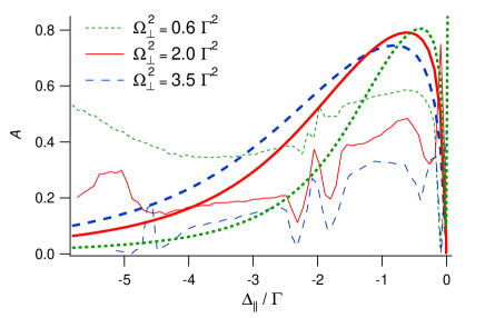
Figure 5: $A$ parameter versus $\Delta_{\parallel}$ for $\Delta_{\perp}=-2\Gamma$, $I_{\parallel}\simeq 2I_{S}$ and different values of $I_{\perp}$. Parameters are the same as in Fig. 4. Thick curves correspond to theoretical values, while thin curves are the experimental records.

We are now able to calculate $A$ both experimentally with the Eq. 9, and theoretically with Eq. 10. Fig. 5 shows as an example the curves obtained for the same parameters as in Fig. 2 and 4. There is no agreement between the experimental curves and the theoretical ones. The main discrepancy concerns the evolution of the $A$ parameter as $I_{\perp}$ is changed: experimentally, $A$ decreases as $I_{\perp}$ is increased, while it is the contrary in the model. Another major inconsistency lies in the fact that for large detunings, the theoretical evolution of all quantities, i.e. $A$, $\kappa$ (Fig. 6, black bold solid line), $\sigma_{L}$ and $\sigma_{R}$, is monotonic. Such a monotonic evolution cannot explain the disappearance of the atomic cloud for intermediate values of $\Delta_{\parallel}$, as observed in the experiments, neither the re-appearance for larger values.

Thus it is clear that the present model is not able to reproduce the experimental observations. Let us remember that in this model, several known physical phenomena have been neglected. The question is now which of them plays finally a role which has been underestimated. The experimental observations shows that the relative values of $I_{\perp}$ and $I_{\parallel}$ play a crucial role in the evolution of both the ellipticity and the number of atoms. As in the present model, the 3D MOT is approximated to three perpendicular independent 1D MOTs, such effects can not be found. Thus it seems logical to enhance the present model to take into account the cross intensity effects between the parallel and transverse beams, and in particular the cross saturation effects. In the next section, we modify the standard model to take into account these effects.

3.3 Introduction of couplings between MOT arms

In the above model, the expression of the parameters $\sigma_{R}$, $\sigma_{L}$ and $\boldsymbol{\kappa}$ result from a 1D approximation. We would like here to enhance this model to take into account, at least partly, the effects induced by the couplings of each pair of beams with its transverse ones. Building a real 3D model would be rather complex. An intermediate model consists in still considering three 1D MOTs, but to introduce for each beam a correction induced by the two other pairs of beams. However, considering the effects of the transverse beams implies in our case to study the excitation of the atomic transition by two quasi-resonant fields with similar amplitudes. The theoretical description of this problem is still laborious. However, it can be greatly simplified for the parallel direction. Indeed, in this case, the two transverse beams have the same frequency, and we can still simplify the model if we consider that the four transverse beams are linearly polarized along $z$ rather than circularly polarized. In this case, the $\sigma^{+}-\sigma^{-}$ longitudinal beams interact with the $\left|m=\pm 1\right\rangle$ levels, while the transverse beams, $\pi$ polarized, interact only with the $\left|m=0\right\rangle$ level. In this case, the calculations can be done in the same way as in romain2011 . The resulting expressions are rather complex and their expressions are useless to understand the underlying physics. However, we expect that, as the fundamental level is now coupled to the $\left|m=0\right\rangle$ level, the number of atoms susceptible to absorb the $\sigma^{+}-\sigma^{-}$ photons is smaller. This should lead to a decreasing of the absorption cross section, and it is effectively what we observed.

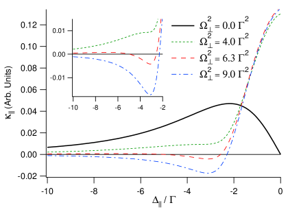
Figure 6: Plot of $\kappa_{\parallel}$ versus $\Delta_{\parallel}$ for different values of $\Omega_{\perp}^{2}$. Parameters are $\Delta_{\perp}=-2\Gamma$ and $\Omega_{\parallel}^{2}=9\Gamma^{2}$.

How the evolution of the spring constant is changed when the transverse coupling is taken into account is more difficult to predict intuitively. And indeed, this evolution is more complex, as shown on Fig. 6, where the values of $\kappa_{\parallel}$ are plotted versus $\Delta_{\parallel}$ for different values of $I_{\perp}$. When $I_{\perp}$ is taken into account, the shape of the curve changes radically. First, because of the coupling, the spring constant is no more zero when the parallel beam is at resonance. For small $I_{\perp}$ (Fig. 6, green dotted line), $\kappa_{\parallel}$ is always positive, and the atoms are trapped whatever $\Delta_{\parallel}$. Thus when the detuning is increased, the cloud population decreases monotonically until it vanishes for large detuning. For larger $I_{\perp}$ (red dashed line), $\kappa_{\parallel}$ becomes negative for intermediate values of $\Delta_{\parallel}$, and becomes positive again for large detuning. In the interval where $\kappa_{\parallel}$ is negative, the atoms are repelled from the trap, and thus for these intermediate detunings, the atomic cloud disappears, but re-appears at large detunings. Finally, for even larger $I_{\perp}$ (blue dotted dashed line), $\kappa_{\parallel}$ becomes negative for intermediate values of $\Delta_{\parallel}$, and remains negative for large detunings: the cloud disappears for rather small $\Delta_{\parallel}$. This behavior is fully consistent with the experimental observations, and thus we can already say that the introduction of cross saturation effects allows us to explain the behavior of an anisotropic trap.

Note also on Fig. 6, the value of the spring constant is also changed for the balanced single-frequency trap: it is for example decreased by a factor 2.6 for $\Delta_{\parallel}=-2\Gamma$ and $\Omega_{\parallel}^{2}=\Omega_{\perp}^{2}=9\Gamma^{2}$. This shows that although usually neglected, the transverse couplings between the trap arms could change significantly the trap parameters.

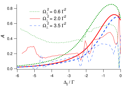
Figure 7: $A$ parameter versus $\Delta_{\parallel}$ for $\Delta_{\perp}=-2\Gamma$, $I_{\parallel}\simeq 2I_{S}$ and different values of $I_{\perp}$. Parameters are the same as in Fig. 5.

We also noticed in section 3.1 that the standard model was unable to reproduce the global evolution of the ellipticities when the transverse intensities are changed. To check that point, we plotted the same curves as in Fig. 5, but for the cross saturation model (Fig. 7). The global evolution of the ellipticities, both theoretical and experimental, are now qualitatively consistent. In particular, when $I_{\perp}$ increases, $A$ decreases in both cases.

4 Conclusion

In this paper, we study the behavior of a dual frequency anisotropic MOT. Experimental measurements show several counter-intuitive behaviors, in particular an interval of detunings where atoms are no more trapped, while they are trapped for smaller and larger detunings. We show that the usual model, which neglects the cross saturation effects, is unable to explain this behavior. We build a model taking into account these cross saturation effects, and show that this model leads to behaviors similar to the experimental ones. The agreement between the experiments and the model is only qualitative. It is not surprising, as numerous approximations remain in the new model. However, it shows that cross saturation effects play a key role in this system.

We also show that even in the traditional balanced single-frequency trap, the couplings between the different arms of the trap change significantly the trap characteristics. As a consequence, these effects should be taken into account when a detail understanding is required.

The coupling between the different directions of the trap also makes it difficult to separate the dynamics of the MOT along the different directions. Thus confining the instabilities of the 3D MOT in only one direction appears to be unrealistic, and a full 3D dynamical model of the MOT seems now necessary.

References

- (1) L. Guidoni and P. Verkerk, J. Opt. B: Quantum Semiclass. Opt. 1 R23 (1999)
- (2) Cold Molecules: Theory, Experiment, Applications, edited by Roman Krems, Bretislav Friedrich and William C. Stwalley (CRC Press, Boca Raton, 2009)
- (3) M. H. Anderson, J. R. Ensher, M. R. Matthews, C. E. Wieman and E. A. Cornell, Science 269 198-201 (1995)
- (4) D. Wilkowski, J. Ringot, D. Hennequin and J. C. Garreau, Phys. Rev. Lett. 85 1839-1842 (2000)
- (5) G. Labeyrie, F. Michaud and R. Kaiser, Phys. Rev. Lett. 96, 023003 (2006)
- (6) D. Hennequin, Eur. Phys. J. D 28 135-147 (2004)
- (7) A. di Stefano, M. Fauquembergue, P. Verkerk and D. Hennequin, Phys. Rev. A 67 033404 (2003)
- (8) A. di Stefano, P. Verkerk and D. Hennequin, Eur. Phys. J. D 30 243-258 (2004)
- (9) T. Pohl, G. Labeyrie, and R. Kaiser, Phys. Rev. A 74, 023409 (2006)
- (10) J. T. Mendonça, R. Kaiser, H. Terças, and J. Loureiro, Phys. Rev. A 78, 013408 (2008)
- (11) R. Romain, D. Hennequin, and P. Verkerk, Eur. Phys. J. D 61, 171–180 (2011)
- (12) M. Vengalattore, W. Rooijakkers, R. Conroy, and M. Prentiss, Phys. Rev. A 67, 063412 (2003)
- (13) Ronald Stites, Michael McClimans, Samir Bali, Optics Communications 248, 173 (2005)
- (14) D. Grison, B. Lounis, C. Salomon, J. Y. Courtois, G. Grynberg, Europhys. Lett. 15, 149-154 (1991)
- (15) D.W. Sesko, T.G. Walker, and C. Wieman, J. Opt. Soc. Am. B 8 946 (1991)
- (16) J. Dalibard, S. Reynaud and C. Cohen-Tannoudji, J. Phys. B: At. Mol. Phys. 17 4577-4594 (1984)