Mean Field Variational Bayesian Inference for
Support Vector Machine Classification

Abstract

A mean field variational Bayes approach to support vector machines (SVMs) using the latent variable representation on Polson & Scott (2012) is presented. This representation allows circumvention of many of the shortcomings associated with classical SVMs including automatic penalty parameter selection, the ability to handle dependent samples, missing data and variable selection. We demonstrate on simulated and real datasets that our approach is easily extendable to non-standard situations and outperforms the classical SVM approach whilst remaining computationally efficient.

1 Introduction

Support vector machines (SVMs) and its variants remain one of the most popular classification methods in machine learning and has been successfully utilized in many applications. Such applications include image classification, speech recognition, cancer diagnosis, natural language processing, forecasting, bio-informatics and as such these methods are likely to remain popular for many years to come. The strengths of SVMs derive from its formulation as an elegant convex optimization problem which can be efficiently solved, has few tuning parameters and whose solution only depends on a subset of the input samples, called support vectors.

Despite such popularity standard SVMs suffer from several shortcomings. Section 10.7 of Hastie et al. (2009) summarize these as: (i) natural handling data of mixed type, (ii) handling of missing values (iii) robustness to outliers in input space (iv) insensitive to monotonic transformations of inputs (v) computational scalability to large sample sizes, (vi) inability to deal with irrelevant inputs and (vii) intepretability. To this list we would add (viii) the inability to deal with correlation within samples. In this paper we aim to address (ii), (vi) and (viii).

This paper is not the first to consider these problems. Missingness has been considered by Smola et al. (2005), Pelckmans et al. (2005) and Nebot-Troyano and Belanche-Muñoz (2010). Dealing with irrelevant inputs via variable/feature selection in SVMs has been considered by many authors including Weston et al. (2000), Tipping (2001), Guyon et al. (2002), Zhu et al. (2003), Gold et al. (2005) and Chu et al. (2006). On the other hand, very few papers consider modification of SVMs to handle dependent or non-identically distributed data. Notable exceptions include Dundar et al. (2007), Lu et al. (2011), Pearce and Wand (2009) and Luts et al. (2012). However, these problems are dealt with in isolation and using different approaches, rather than in a unified manner and it is difficult to see how these approaches could be adapted to multiple complications, e.g., missingness and variable selection.

In the paper we follow the earlier work of Boser et al. (1992), Bishop and Tipping (2000), Gao and Wong (2005) and Polson and Scott (2011) who propose various latent variable representations of the SVM loss function and reformulate the problem in a (pseudo-) Bayesian framework. This provides a unified approach which releases SVMs from many of the above problems including allowing efficient penalty parameter selection, correlation within samples, variable selection and missing data via well developed Bayesian methodology. Typically such Bayesian models are fit via Markov chain Monte Carlo (MCMC) methods. Unfortunately, MCMC methods can be notoriously slow when applied to large or complex models and can be rendered unsuitable in applications where speed is essential. These situations are precisely the same situations where SVMs are typically popular.

Our approach to this problem is to apply mean field variational Bayes (VB) methods to the models we propose. The main advantage of this approach is a streamlined and computationally efficient framework for handling to many of the problems associated with the classical SVM approach. In tandem with these algorithms we also develop Gibbs sampling approaches to these methods to facilitate comparisons with an “exact” approach to these models.

In Section 2 we provide the framework for our approach. In Section 3 we consider various extensions including automatic penalty parameter selection, group correlations, variable selection and missing predictors respectively. In Section 4 we show how our approach offers several computational advantages over the classical SVM approach. In Section 5 we conclude. Appendices contain details of our MCMC samplers.

Notation

The notation $\boldsymbol{x}\sim N(\boldsymbol{\mu},\boldsymbol{\Sigma})$ means that $\boldsymbol{x}$ has a multivariate normal density with mean $\boldsymbol{\mu}$ and covariance $\boldsymbol{\Sigma}$. If $x$ has an inverse gamma distribution, denoted $x\sim\mbox{IG}(A,B)$, then it has density $p(x)=B^{A}\Gamma(A)^{-1}x^{-A-1}\exp(-B/x)$, $x,A,B>0$. If $x$ has an inverse Gaussian distribution, denoted
$x\sim\mbox{Inverse-Gaussian}(\mu,\lambda)$ with mean $\mu$ and variance $\mu^{3}/\lambda$, then it has density

$$p(x)=\sqrt{\frac{\lambda}{2\pi x^{3}}}\exp\left\{-\frac{\lambda(x-\mu)^{2}}{2x\mu^{2}}\right\},\quad x,\mu,\lambda>0.$$

If $x$ has a generalized inverse Gaussian distribution, denoted $x\sim\mbox{GIG}(\gamma,\psi,\chi)$, then it has density

$$p(x)=\frac{(\psi/\chi)^{\gamma/2}}{2K_{\gamma}(\sqrt{\psi\chi})}x^{\gamma-1}\exp\left\{-\frac{1}{2}\left(\frac{\chi}{x}+\psi x\right)\right\},\quad x,\psi,\chi>0,\ \gamma\in\mathbb{R},$$

where $K_{\gamma}(\cdot)$ is a modified Bessel function of the second kind. If $\boldsymbol{x}$ is a vector of length $d$ then $\mbox{diag}(\boldsymbol{x})$ is the $d\times d$ diagonal matrix whose diagonal elements are $\boldsymbol{x}$. If $\boldsymbol{X}$ is a $d\times d$ matrix then $\mbox{dg}(\boldsymbol{X})$ is the vector of length $d$ comprising of the diagonal elements of $\boldsymbol{X}$. The $j$th column of a matrix ${\bf X}$ is denoted ${\bf X}_{j}$.

2 Methodology

In this section we present a VB approach to a Bayesian SVM classification formulation for binary classification problems. After introducing Bayesian SVMs and VB methodology we describe the latent variable SVM representation of Polson and Scott (2011) which gives rise to our basic VBSVM approach.

2.1 Bayesian support vector machines

Consider a training set $\{y_{i},\boldsymbol{x}_{i}\}_{i=1}^{n}$, where $\boldsymbol{x}_{i}\in\mathbb{R}^{p}$ represents an input vector and $y_{i}\in\{-1,+1\}$ the corresponding class label. SVMs can be formulated in terms of finding a linear hyperplane that separates the observations with $y_{i}=1$ from those with $y_{i}=-1$ with the largest minimal separating distance or margin. In general such a hyperplane does not exist and the problem needs to be reformulated as a trade-off between the size of the margin and infringements caused by points being on the wrong side of the hyperplane (for more details see for example Vapnik (1998) or Chapter 12 of Hastie et al. (2009)). This optimization problem amounts to finding $\boldsymbol{\beta}\in\mathbb{R}^{p}$ which minimizes

$$\min_{\boldsymbol{\beta}}{\mathcal{J}}(\boldsymbol{\beta})=\left\{\sum_{i=1}^{n}(1-y_{i}\boldsymbol{x}_{i}^{T}\boldsymbol{\beta})_{+}\right\}+\alpha\|\boldsymbol{\beta}\|^{2},$$ (1)

where $\alpha$ is a positive penalty parameter (the choice of which we will discuss later) and $x_{+}=\max(0,x)$. Larger values of $\alpha$ serve to shrink the fitted values of the $\boldsymbol{\beta}$ coefficients. The above problem can be reformulated as a convex quadratic programming problem and can be solved using a variety of efficient methods (for example Chapter 7 of Cristianini and Shawe-Taylor (2000)). This results in the classification rule $\mbox{sign}(\boldsymbol{x}_{i}^{T}\boldsymbol{\beta})$ for input vector $\boldsymbol{x}_{i}$.

The terms $(1-y_{i}\boldsymbol{x}_{i}^{T}\boldsymbol{\beta})_{+}$ in (1) are referred to as the hinge loss of the data and using a logarithmic scoring rule interpretation (Bernardo, 1979) can be interpreted as negative conditional log-likelihoods. This has motivated Bayesian SVM formulations where

$$p\ell(y_{i}|\boldsymbol{\beta})=\exp\left\{-(1-y_{i}\boldsymbol{x}_{i}^{T}\boldsymbol{\beta})_{+}\right\},\ 1\leq i\leq n,\quad\mbox{and}\quad\boldsymbol{\beta}\sim N(\boldsymbol{0},\tfrac{1}{2}\alpha^{-1}\boldsymbol{I}_{p}),$$ (2)

where $p\ell(y_{i}|\boldsymbol{\beta})$ is the pseudo-likelihood contribution of the $i$th observation. Although (2) is not a true likelihood for the remainder of the paper we will ignore this distinction and write $p\ell(y_{i}|\boldsymbol{\beta})$ as $p(y_{i}|\boldsymbol{\beta})$. Then

$$p(\boldsymbol{y},\boldsymbol{\beta})=p(\boldsymbol{\beta})\prod_{i=1}^{n}p(y_{i}|\boldsymbol{\beta})\propto\exp\{-{\mathcal{J}}(\boldsymbol{\beta})\},$$

where $\boldsymbol{y}=[y_{1},\ldots,y_{n}]^{T}$. Following Mallick et al. (2005) we refer to formulations taking into account the normalizing constant of $p(\boldsymbol{y},\boldsymbol{\beta})$ as complete SVM (CSVM) formulations whereas formulations ignoring the normalizing constant as Bayesian SVM (BSVM) formulations. We only consider the BSVM formulations here, i.e. (2).

Lastly, nonlinear classifiers can be constructed using kernelization methods (see for example Zhang et al. (2011)).

2.2 Variational Bayesian inference

As discussed in the introduction the advantage of the Bayesian formulation is that it allows us to extend SVM methodology to handle a variety of complications. Such Bayesian formulations are typically fit using MCMC approaches (Mallick et al., 2005; Polson and Scott, 2011; Zhang et al., 2011). Unfortunately, MCMC approaches are often slow for the data mining applications where SVMs are typically used.

Mean field variational Bayes is a class of methods for approximate Bayesian inference which are typically much faster than MCMC methods. Consider the set of data ${\mathcal{D}}$ described by the joint likelihood $p({\mathcal{D}},\boldsymbol{\theta})$ where $\boldsymbol{\theta}$ is a vector of parameters, latent variables or missing values. Then it can be shown for a density of the form $q(\boldsymbol{\theta})=\prod_{i=1}^{K}q_{i}(\boldsymbol{\theta}_{i})$ that the optimal $q_{i}^{*}(\boldsymbol{\theta}_{i})$, which minimize the Kullback-Leibler distance between $q(\boldsymbol{\theta})$ and $p(\boldsymbol{\theta}|{\mathcal{D}})$, satisfy

$$q_{i}^{*}(\boldsymbol{\theta}_{i})\propto\exp\left[\mathbb{E}_{-q(\boldsymbol{\theta}_{i})}\left\{\log p({\mathcal{D}},\boldsymbol{\theta})\right\}\right]$$ (3)

where $\mathbb{E}_{-q(\boldsymbol{\theta}_{i})}$ denotes expectations over $\prod_{j\neq i}q_{j}^{*}(\boldsymbol{\theta}_{j})$. If (3) is calculated iteratively over $i$ then the lower bound on the marginal log-likelihood

$$\log\underline{p}({\mathcal{D}};q)=\mathbb{E}_{q(\boldsymbol{\theta})}\left[\log\left\{\frac{p({\mathcal{D}},\boldsymbol{\theta})}{q(\boldsymbol{\theta})}\right\}\right]$$ (4)

is guaranteed to increase monotonically. For more details and examples see Bishop (2006) or Ormerod and Wand (2010).

2.3 Variational Bayesian support vector machines

Polson and Scott (2011) formulated an auxiliary variable representation of the problem analogous to (1), where the hinge loss is represented by a location-scale mixture of normal distributions. While Mallick et al. (2005) also consider an auxiliary representation of the SVM we use the representation of Polson and Scott (2011) because the calculation of (3) and (4) are analytically tractable.

Specifically, let

$$p(y_{i},a_{i}|\boldsymbol{\beta})=\frac{1}{\sqrt{2\pi a_{i}}}\exp\left[-\frac{(1+a_{i}-y_{i}\boldsymbol{x}_{i}^{T}\boldsymbol{\beta})^{2}}{2a_{i}}\right],$$

where the $a_{i}>0$ values are auxiliary variables. Then the data augmentation approach of Polson and Scott (2011) uses the fact that

$$\exp[-2(1-y_{i}\boldsymbol{x}_{i}^{T}\boldsymbol{\beta})_{+}]=\int_{0}^{\infty}p(y_{i},a_{i}|\boldsymbol{\beta})da_{i}.$$

Hence, if $\boldsymbol{\beta}\sim N(\boldsymbol{0},\tfrac{1}{4}\alpha^{-1}\boldsymbol{I}_{p})$ then

$$\log p(\boldsymbol{\beta})+\sum_{i=1}^{n}\left[\log\int_{0}^{\infty}p(y_{i},a_{i}|\boldsymbol{\beta})da_{i}\right]\propto-2{\mathcal{J}}(\boldsymbol{\beta}).$$

Instead of performing inference on the parameter vector $\boldsymbol{\beta}$ we treat $\boldsymbol{a}=[a_{1},\ldots,a_{n}]^{T}$ as random and perform inference on $\boldsymbol{\theta}=[\boldsymbol{\beta}^{T},\boldsymbol{a}^{T}]^{T}$. The main advantage of this representation is that the pseudo-conditional distribution $p(\boldsymbol{y},\boldsymbol{a}|\boldsymbol{\beta})=\prod_{i=1}^{n}p(y_{i},a_{i}|\boldsymbol{\beta})$ is conjugate to a multivariate normal distribution.

Our proposed VB approach uses this representation of $p(\boldsymbol{y},\boldsymbol{a}|\boldsymbol{\beta})$ combined with the posterior density restriction

$$q(\boldsymbol{\beta},\boldsymbol{a})=q(\boldsymbol{\beta})\prod_{i=1}^{n}q(a_{i}).$$

The resulting $q$-densities which minimize the Kullback-Leibler distance between $q(\boldsymbol{a},\boldsymbol{\beta})$ and the posterior densities are of the form

$$q^{*}(\boldsymbol{\beta})\displaystyle\sim N(\boldsymbol{\mu}_{q(\boldsymbol{\beta})},\boldsymbol{\Sigma}_{q(\boldsymbol{\beta})})\quad\mbox{and}\quad q^{*}(a_{i})\stackrel{{\scriptstyle{\tiny\mbox{ind.}}}}{{\sim}}\mbox{GIG}\left(\tfrac{1}{2},1,\chi_{q(a_{i})}\right),\quad 1\leq i\leq n,$$

where

$$\begin{array}[]{c}\boldsymbol{\Sigma}_{q(\boldsymbol{\beta})}=\left(\boldsymbol{X}^{T}\mbox{diag}(\boldsymbol{\mu}_{q(\boldsymbol{a}^{-1})})\boldsymbol{X}+4\alpha\boldsymbol{I}_{p}\right)^{-1},\quad\boldsymbol{\mu}_{q(\boldsymbol{\beta})}=\boldsymbol{\Sigma}_{q(\boldsymbol{\beta})}\boldsymbol{X}^{T}\boldsymbol{Y}(\boldsymbol{1}_{n}+\boldsymbol{\mu}_{q(\boldsymbol{a}^{-1})}),\\ \chi_{q(a_{i})}=(1-y_{i}\boldsymbol{x}_{i}^{T}\boldsymbol{\mu}_{q(\boldsymbol{\beta})})^{2}+\boldsymbol{x}_{i}^{T}\boldsymbol{\Sigma}_{q(\boldsymbol{\beta})}\boldsymbol{x}_{i}\quad\mbox{and}\quad\mu_{q(a_{i}^{-1})}=\chi_{q(a_{i})}^{-1/2},\ 1\leq i\leq n.\end{array}$$

In the above expressions $\boldsymbol{X}$ denotes the $n$ by $p$ matrix such that the $i$th row of $\boldsymbol{X}$ is $\boldsymbol{x}_{i}$ and $\boldsymbol{Y}=\mbox{diag}(\boldsymbol{y})$. In order to reduce the length of later expressions we let $\boldsymbol{W}=\mbox{diag}(\boldsymbol{\mu}_{q(\boldsymbol{a}^{-1})})$. The parameters $\boldsymbol{\mu}_{q(\boldsymbol{\beta})}$, $\boldsymbol{\Sigma}_{q(\boldsymbol{\beta})}$ and $\chi_{q(a_{i})}$ are determined by Algorithm 1. In Algorithm 1 the symbol $\odot$ denotes element-wise multiplication.

Convergence of Algorithm 1 is monitored using the variational lower bound on the marginal likelihood, i.e., $\log\underline{p}(\boldsymbol{y};q)$ given by

$$\begin{array}[]{rl}\log\underline{p}(\boldsymbol{y};q)&\displaystyle=\tfrac{p}{2}-n+n\log(2)-\tfrac{n}{2}\log(2\pi)+\tfrac{p}{2}\log(4\alpha)+\tfrac{1}{2}\log|\boldsymbol{\Sigma}_{q(\boldsymbol{\beta})}|-2\alpha\left[\|\boldsymbol{\mu}_{q(\boldsymbol{\beta})}\|^{2}+\mbox{tr}(\boldsymbol{\Sigma}_{q(\boldsymbol{\beta})})\right]\\ &\displaystyle\quad+\boldsymbol{y}^{T}\boldsymbol{X}\boldsymbol{\mu}_{q(\boldsymbol{\beta})}+\tfrac{1}{4}\boldsymbol{1}_{n}^{T}\log(\boldsymbol{\chi}_{q({\boldsymbol{a}})})+\boldsymbol{1}_{n}^{T}\log K_{1/2}(\sqrt{\boldsymbol{\chi}_{q({\boldsymbol{a}})}}).\end{array}$$

Algorithm 1 Iterative scheme for obtaining the parameters in the optimal densities $q^{*}(\boldsymbol{\beta})$ and $q^{*}(\boldsymbol{a})$ for the variational Bayesian support vector machine with $\alpha$ fixed.

0:  $\boldsymbol{\mu}_{q({\boldsymbol{a}^{-1}})}>\boldsymbol{0}$

1:  while the increase in $\log\underline{p}(\boldsymbol{y};q)$ is significant do

2:     $\boldsymbol{W}\leftarrow\mbox{diag}(\boldsymbol{\mu}_{q(\boldsymbol{a}^{-1})})\quad;\quad\boldsymbol{\Sigma}_{q(\boldsymbol{\beta})}\leftarrow\left(\boldsymbol{X}^{T}\boldsymbol{W}\boldsymbol{X}+4\alpha\boldsymbol{I}_{p}\right)^{-1}\quad;\quad\boldsymbol{\mu}_{q(\boldsymbol{\beta})}\leftarrow\boldsymbol{\Sigma}_{q(\boldsymbol{\beta})}\boldsymbol{X}^{T}(\boldsymbol{I}_{n}+\boldsymbol{W})\boldsymbol{y}$

3:     $\boldsymbol{\chi}_{q({\boldsymbol{a}})}\leftarrow(\boldsymbol{1}_{n}-\boldsymbol{Y}\boldsymbol{X}\boldsymbol{\mu}_{q(\boldsymbol{\beta})})^{2}+\mbox{dg}(\boldsymbol{X}\boldsymbol{\Sigma}_{q(\boldsymbol{\beta})}\boldsymbol{X}^{T})\quad;\quad\boldsymbol{\mu}_{q({\boldsymbol{a}^{-1}})}\leftarrow\boldsymbol{\chi}_{q({\boldsymbol{a}})}^{-1/2}$

4:  end while

3 Extensions

We now present a number of extensions addressing some of the shortcomings of SVMs. These are presented in increasing complexity.

3.1 Penalty parameter inference and random effect models

Note that the positive penalization constant $\alpha$ in the previous section remains unspecified. By choosing an appropriate value for the constant $\alpha$ in (1), the objective function trades the loss term against the $\|\boldsymbol{\beta}\|^{2}$ penalty term. This restricts the space of solutions, reduces the effect of overfitting and allows generalization to new, unseen data. Popular approaches for tuning the penalty parameter include cross-validation techniques and random sampling methods. However, these approaches to selecting $\alpha$ increase the overall computational overhead of these methods.

One approach to selecting the penalty parameter is by embedding a model into a mixed effect framework. Such an approach is commonly used to select the penalty parameter in penalized spline methods (Wand, 2003; Wand and Ormerod, 2008), the main by-product of which is enabling a natural embedding of semiparametric regression structures into SVM models (Ruppert et al., 2003; Zhao et al., 2006).

We now show how the basic VBSVM model can be easily extended for selecting the penalty parameter automatically (without the need of a cross-validation strategy) and simultaneously how to handle group dependent data via a random intercept model. Let

$$\begin{array}[]{rl}\displaystyle p(\boldsymbol{y},\boldsymbol{a}|\boldsymbol{\beta},\boldsymbol{u})&\displaystyle=\exp\Big{[}-n-\tfrac{n}{2}\log(2\pi)-\tfrac{1}{2}\boldsymbol{1}_{n}^{T}\log(\boldsymbol{a})-\tfrac{1}{2}\boldsymbol{1}_{n}^{T}(\boldsymbol{a}+\boldsymbol{a}^{-1})\\ &\displaystyle\qquad+(\boldsymbol{1}_{n}+\boldsymbol{a}^{-1})^{T}\boldsymbol{Y}(\boldsymbol{X}\boldsymbol{\beta}+\boldsymbol{Z}\boldsymbol{u})-\tfrac{1}{2}(\boldsymbol{X}\boldsymbol{\beta}+\boldsymbol{Z}\boldsymbol{u})^{T}\mbox{diag}(\boldsymbol{a}^{-1})(\boldsymbol{X}\boldsymbol{\beta}+\boldsymbol{Z}\boldsymbol{u})\Big{]}\\ \quad\displaystyle\mbox{and}\quad\boldsymbol{u}|\boldsymbol{\Sigma}&\displaystyle\sim N(\boldsymbol{0}_{m},\boldsymbol{\Sigma}),\end{array}$$ (5)

where $\boldsymbol{X}\in\mathbb{R}^{n\times p}$ and $\boldsymbol{Z}\in\mathbb{R}^{n\times m}$ are fixed and random effect design matrices respectively and $\boldsymbol{\Sigma}$ is the covariance of $\boldsymbol{u}$. This class of models is extremely rich allowing random intercept, random slope, cross random effects, nested random effects, smoothing, generalized additive and semiparametric structures (Zhao et al., 2006). We will consider the following two examples.

Example 1 [Penalty parameter selection]: Consider the data matrix $\boldsymbol{D}\in\mathbb{R}^{n\times d}$ containing our observed predictors, i.e., $D_{ij}$ is the $i$th sample of the $j$th predictor. Suppose we wish to penalize the size of the coefficients associated with these predictors, but do not wish to penalize the size of the intercept coefficient. Then we would choose

$$\boldsymbol{X}=\boldsymbol{1}_{n},\quad\boldsymbol{Z}=\boldsymbol{D}\quad\mbox{and}\quad\boldsymbol{\Sigma}=\sigma_{u}^{2}\boldsymbol{I}_{m}$$

where $p=1$, $m=d$ and $\sigma_{u}^{2}=\frac{1}{4}\alpha^{-1}$.

Example 2 [Random intercept]: Suppose we have the data $\{y_{i,j},{\bf d}_{i,j}\}$, $1\leq i\leq m$, $1\leq j\leq n_{i}$ where $m$ is the number of groups, $n_{i}$ is the number of observations in group $i$ and ${\bf d}_{i,j}\in\mathbb{R}^{d}$. Then we would define $n=\sum_{i=1}^{m}n_{i}$ and choose

$$\boldsymbol{y}=\left[\begin{array}[]{c}y_{1,1}\\ \vdots\\ y_{1,n_{1}}\\ y_{2,1}\\ \vdots\\ y_{m,n_{m}}\\ \end{array}\right],\quad\boldsymbol{X}=\left[\begin{array}[]{cc}1&{\bf d}_{1,1}^{T}\\ \vdots&\vdots\\ 1&{\bf d}_{1,n_{1}}^{T}\\ 1&{\bf d}_{2,1}^{T}\\ \vdots&\vdots\\ 1&{\bf d}_{m,n_{m}}^{T}\\ \end{array}\right],\quad\boldsymbol{Z}=\left[\begin{array}[]{cccc}\boldsymbol{1}_{n_{1}}&\boldsymbol{0}_{n_{1}}&\cdots&\boldsymbol{0}_{n_{1}}\\ \boldsymbol{0}_{n_{2}}&\boldsymbol{1}_{n_{2}}&\cdots&\boldsymbol{0}_{n_{2}}\\ \vdots&\vdots&\ddots&\vdots\\ \boldsymbol{0}_{n_{m}}&\boldsymbol{0}_{n_{m}}&\cdots&\boldsymbol{1}_{n_{m}}\\ \end{array}\right]\quad\mbox{and}\quad\boldsymbol{\Sigma}=\sigma_{u}^{2}\boldsymbol{I}_{m}$$

where $p=d+1$ and $\sigma_{u}^{2}$ is the random intercept variance.

For both these examples we use the priors

$$\boldsymbol{\beta}\sim N({\bf 0}_{p},\sigma_{\beta}^{2}\boldsymbol{I}_{p})\quad\mbox{and}\quad\sigma_{u}^{2}\sim\mbox{IG}(A_{u},B_{u})$$

where $\sigma_{\beta}^{2}$, $A_{u}$ and $B_{u}$ are fixed prior hyperparameters. For our numerical experiments we use the values $\sigma_{\beta}^{2}=10^{8}$ and $A_{u}=B_{u}=0.01$ as defaults to impose non-informativity. Placing a prior on $\sigma_{u}^{2}=\alpha^{-1}/4$ allows us to perform inference on the penalty parameter.

To apply the VB method we choose the product restriction for approximating the posterior density of the form

$$q(\boldsymbol{\beta},\boldsymbol{u},\sigma_{u}^{2},\boldsymbol{a})=q(\boldsymbol{\beta},\boldsymbol{u})q(\sigma_{u}^{2})\prod_{i=1}^{n}q(a_{i}).$$

Using (3) and this product restriction the optimal $q$-densities are of the form

$$\begin{array}[]{c}\displaystyle q^{*}(\boldsymbol{\beta},\boldsymbol{u})\displaystyle\sim N(\boldsymbol{\mu}_{q(\boldsymbol{\beta},\boldsymbol{u})},\boldsymbol{\Sigma}_{q(\boldsymbol{\beta},\boldsymbol{u})}),\quad q^{*}(\sigma_{u}^{2})\displaystyle\sim\mbox{IG}\left(A_{u}+\tfrac{m}{2},B_{q(\sigma_{u}^{2})}\right)\\ \mbox{and}\quad q^{*}(a_{i})\stackrel{{\scriptstyle{\tiny\mbox{ind.}}}}{{\sim}}\mbox{GIG}\left(\tfrac{1}{2},1,\chi_{q(a_{i})}\right),\quad 1\leq i\leq n,\end{array}$$

where the parameters are determined by Algorithm 2. In Algorithm 2 the matrix $\boldsymbol{C}$ is $[\boldsymbol{X},\boldsymbol{Z}]$ and in the main loop the lower bound on the marginal log-likelihood simplifies to

$$\begin{array}[]{rl}\displaystyle\log\underline{p}(\boldsymbol{y};q)&\displaystyle=\tfrac{p+m}{2}-n+n\log(2)-\tfrac{n}{2}\log(2\pi)-\tfrac{p}{2}\log(\sigma_{\beta}^{2})+\tfrac{1}{2}\log|\boldsymbol{\Sigma}_{q(\boldsymbol{\beta},\boldsymbol{u})}|-\tfrac{1}{2\sigma_{\beta}^{2}}\left[\|\boldsymbol{\mu}_{q(\boldsymbol{\beta})}\|^{2}+\mbox{tr}(\boldsymbol{\Sigma}_{q(\boldsymbol{\beta})})\right]\\ &\displaystyle\quad+A_{u}\log(B_{u})-\log\Gamma(A_{u})-\left(A_{u}+\tfrac{m}{2}\right)\log(B_{q(\sigma_{u}^{2})})+\log\Gamma\left(A_{u}+\tfrac{m}{2}\right)\\ &\displaystyle\quad+\boldsymbol{y}^{T}\boldsymbol{C}\boldsymbol{\mu}_{q(\boldsymbol{\beta},\boldsymbol{u})}+\tfrac{1}{4}\boldsymbol{1}_{n}^{T}\log(\boldsymbol{\chi}_{q({\boldsymbol{a}})})+\boldsymbol{1}_{n}^{T}\log K_{1/2}(\sqrt{\boldsymbol{\chi}_{q({\boldsymbol{a}})}}),\end{array}$$

where $\Gamma(\cdot)$ is the gamma function. Classification of a new input vector $\boldsymbol{c}_{i}$ is performed based on the value $\text{sign}(\boldsymbol{c}_{i}^{T}\boldsymbol{\mu}^{*}_{q(\boldsymbol{\beta},\boldsymbol{u})})$.

Algorithm 2 Iterative scheme for obtaining the parameters in the optimal densities $q^{*}(\boldsymbol{\beta},\boldsymbol{u})$, $q^{*}(\sigma_{u}^{2})$ and $q^{*}(\boldsymbol{a})$ for the variational Bayesian support vector machine with penalty parameter or random intercept inference.

0:  $\boldsymbol{\mu}_{q({\boldsymbol{a}^{-1}})}>\boldsymbol{0}_{n},\mu_{q({\sigma_{u}^{-2}})}>0$

1:  while the increase in $\log\underline{p}(\boldsymbol{y};q)$ is significant do

2:     $\boldsymbol{W}\leftarrow\mbox{diag}(\boldsymbol{\mu}_{q({\boldsymbol{a}^{-1}})})\quad;\quad\boldsymbol{\Sigma}_{q(\boldsymbol{\beta},\boldsymbol{u})}\leftarrow\left[\boldsymbol{C}^{T}\boldsymbol{W}\boldsymbol{C}+\mbox{blockdiag}(\sigma_{\beta}^{-2}\boldsymbol{I}_{p},\mu_{q({\sigma_{u}^{-2}})}\boldsymbol{I}_{m})\right]^{-1}$

3:     $\boldsymbol{\mu}_{q(\boldsymbol{\beta},\boldsymbol{u})}\leftarrow\boldsymbol{\Sigma}_{q(\boldsymbol{\beta},\boldsymbol{u})}\boldsymbol{C}^{T}(\boldsymbol{I}_{n}+\boldsymbol{W})\boldsymbol{y}\quad;\quad\boldsymbol{\chi}_{q({\boldsymbol{a}})}\leftarrow(\boldsymbol{1}_{n}-\boldsymbol{Y}\boldsymbol{C}\boldsymbol{\mu}_{q(\boldsymbol{\beta},\boldsymbol{u})})^{2}+\mbox{dg}(\boldsymbol{C}\boldsymbol{\Sigma}_{q(\boldsymbol{\beta},\boldsymbol{u})}\boldsymbol{C}^{T})\quad;\quad\boldsymbol{\mu}_{q({\boldsymbol{a}^{-1}})}\leftarrow\boldsymbol{\chi}_{q({\boldsymbol{a}})}^{-1/2}$

4:     $B_{q(\sigma_{u}^{2})}\leftarrow B_{u}+\tfrac{1}{2}\left[\|\boldsymbol{\mu}_{q(\boldsymbol{u})}\|^{2}+\text{tr}(\boldsymbol{\Sigma}_{q(\boldsymbol{u})})\right]\quad;\quad\mu_{q({\sigma_{u}^{-2}})}\leftarrow(A_{u}+m/2)/B_{q(\sigma_{u}^{2})}$

5:  end while

3.2 Variable selection

The classical 2-norm SVM and the VBSVM approaches we have described so far include no mechanism to induce sparsity for the fitted coefficients. Inducing sparsity is important because it allows us to remove potentially irrelevant or redundant variables. In this section we present a VBSVM which overcomes this via the incorporation of a sparse prior. While there exist numerous options for the choice of the sparse prior, we will make use of the Laplace-zero density (Wand and Ormerod, 2011).

Consider again the model (5). Suppose that we wish the fitted $\boldsymbol{\beta}$ be included in the model (which may include terms such as the intercept) whereas we wish to induce sparsity on the vector of fitted $\boldsymbol{u}$. Instead of using $\boldsymbol{u}|\sigma_{u}^{2}\sim N(\boldsymbol{0}_{m},\sigma_{u}^{2}\boldsymbol{I}_{m})$ consider the hierarchical prior for $u_{k}$ given by

$$\begin{array}[]{c}u_{k}|\gamma_{k},\sigma_{u}\stackrel{{\scriptstyle{\tiny\mbox{ind.}}}}{{\sim}}\gamma_{k}\mbox{Laplace}(0,\sigma_{u})+(1-\gamma_{k})\delta_{0},\quad\gamma_{k}|\rho\stackrel{{\scriptstyle{\tiny\mbox{ind.}}}}{{\sim}}\mbox{Bernoulli}(\rho),\quad 1\leq k\leq m,\\ \end{array}$$

where $\delta_{0}$ is the degenerate distribution with point mass at $0$. This representation is unnatural to work with using VB methodology and so we use a more natural representation.

First, we note that the Laplace distribution can be represented using a normal-scale mixture (Andrews and Mallows, 1974). This representation uses the fact that

$$\mbox{if}\quad v_{k}|b_{k},\sigma_{u}^{2}\stackrel{{\scriptstyle{\tiny\mbox{ind.}}}}{{\sim}}N(0,\sigma_{u}^{2}/b_{k})\quad\mbox{and}\quad b_{k}\stackrel{{\scriptstyle{\tiny\mbox{ind.}}}}{{\sim}}\mbox{IG}(1,1/2)\quad\mbox{then}\quad v_{k}|\sigma_{u}\stackrel{{\scriptstyle\mbox{\tiny ind.}}}{{\sim}}\mbox{Laplace}(0,\sigma_{u}).$$

Hence, instead of (5) we let $u_{k}=\gamma_{k}v_{k}$ and use

$$\begin{array}[]{c}\begin{array}[]{rl}\displaystyle p(\boldsymbol{y},\boldsymbol{a}|\boldsymbol{\beta},\boldsymbol{v},\boldsymbol{\gamma})&\displaystyle=\exp\Big{[}-n-\tfrac{n}{2}\log(2\pi)-\tfrac{1}{2}\boldsymbol{1}_{n}^{T}\log(\boldsymbol{a})-\tfrac{1}{2}\boldsymbol{1}_{n}^{T}(\boldsymbol{a}+\boldsymbol{a}^{-1})\\ &\displaystyle\qquad+(\boldsymbol{1}_{n}+\boldsymbol{a}^{-1})^{T}\boldsymbol{Y}(\boldsymbol{X}\boldsymbol{\beta}+\boldsymbol{Z}\boldsymbol{\Gamma}\boldsymbol{v})-\tfrac{1}{2}(\boldsymbol{X}\boldsymbol{\beta}+\boldsymbol{Z}\boldsymbol{\Gamma}\boldsymbol{v})^{T}\mbox{diag}(\boldsymbol{a}^{-1})(\boldsymbol{X}\boldsymbol{\beta}+\boldsymbol{Z}\boldsymbol{\Gamma}\boldsymbol{v})\Big{]},\end{array}\\ \displaystyle\boldsymbol{v}|\boldsymbol{b},\sigma_{u}^{2}\sim N(\boldsymbol{0},\sigma_{u}^{2}\mbox{diag}(\boldsymbol{b}^{-1})),\quad\quad b_{k}\stackrel{{\scriptstyle{\tiny\mbox{ind.}}}}{{\sim}}\mbox{IG}(1,1/2)\quad\mbox{and}\quad\gamma_{k}\stackrel{{\scriptstyle{\tiny\mbox{ind.}}}}{{\sim}}\text{Bernoulli}(\rho),\quad 1\leq k\leq m,\end{array}$$

where $\boldsymbol{b}=[b_{1},\ldots,b_{m}]^{T}$, $\boldsymbol{v}=[v_{1},\ldots,v_{m}]$, $\boldsymbol{\gamma}=[\gamma_{1},\ldots,\gamma_{m}]$ and $\boldsymbol{\Gamma}=\mbox{diag}(\boldsymbol{\gamma})$, and use the priors

$$\boldsymbol{\beta}\sim N(\boldsymbol{0}_{p},\sigma_{\beta}^{2}\boldsymbol{I}_{p})\quad\mbox{and}\quad\quad\sigma_{u}^{2}\sim\mbox{IG}(A_{u},B_{u}).$$

The set of auxiliary variables $\gamma_{k}$ and $b_{k}$ has been introduced such that $u_{k}|\gamma_{k},\sigma_{u}$ has the desired Laplace-zero prior distribution. The hyperparameter $\rho$ is chosen in function of the desired level of sparsity.

Next, a factorization is specified for the approximation to the posterior density function by

$$q(\boldsymbol{\beta},\boldsymbol{v},\sigma_{u}^{2},\boldsymbol{a},\boldsymbol{b},\boldsymbol{\gamma})=q(\boldsymbol{\beta},\boldsymbol{v})q(\sigma_{u}^{2})\left[\prod_{i=1}^{n}q(a_{i})\right]\left[\prod_{k=1}^{m}q(b_{k})q(\gamma_{k})\right].$$

Using (3) and this product restriction the optimal $q$-densities are of the form

$$\begin{array}[]{c}q^{*}(\boldsymbol{\beta},\boldsymbol{v})\sim N(\boldsymbol{\mu}_{q(\boldsymbol{\beta},\boldsymbol{v})},\boldsymbol{\Sigma}_{q(\boldsymbol{\beta},\boldsymbol{v})}),\quad q^{*}(\sigma_{u}^{2})\sim\mbox{IG}\left(A_{u}+\frac{m}{2},B_{q(\sigma_{u}^{2})}\right),\\ q^{*}(b_{k})\stackrel{{\scriptstyle{\tiny\mbox{ind.}}}}{{\sim}}\mbox{Inverse-Gaussian}\left(\mu_{q(b_{k})},1\right),\quad q^{*}(\gamma_{k})\stackrel{{\scriptstyle{\tiny\mbox{ind.}}}}{{\sim}}\mbox{Bernoulli}\left(\mu_{q(\gamma_{k})}\right),\ 1\leq k\leq m,\\ \mbox{and}\quad q^{*}(a_{i})\stackrel{{\scriptstyle{\tiny\mbox{ind.}}}}{{\sim}}\mbox{GIG}(\frac{1}{2},1,\chi_{q(a_{i})}),\ 1\leq i\leq n,\end{array}$$

where the parameters are determined by Algorithm 3. In Algorithm 3 we use the function $\mbox{expit}(x)=1/(1+\exp(-x))$, let $\boldsymbol{Z}_{k}$ denote the $k$th column of $\boldsymbol{Z}$ and let $\boldsymbol{Z}_{-k}$ be the $\boldsymbol{Z}$ matrix with the $k$th column removed. The lower bound in the main loop in Algorithm 3 takes the simplified form

$$\begin{array}[]{rl}\displaystyle\log\underline{p}(\boldsymbol{y};q)&\displaystyle=(n-m)\log(2)-n+\tfrac{p+m}{2}-\tfrac{n-m}{2}\log(2\pi)\\ &\displaystyle\quad+\boldsymbol{y}^{T}\boldsymbol{C}\mbox{diag}(\boldsymbol{\mu}_{q(\widetilde{\boldsymbol{\gamma}})}){\boldsymbol{\mu}}_{q(\boldsymbol{\beta},\boldsymbol{v})}+\tfrac{1}{4}\boldsymbol{1}_{n}^{T}\log(\boldsymbol{\chi}_{q(\boldsymbol{a})})+\boldsymbol{1}_{n}^{T}\log K_{1/2}(\sqrt{\boldsymbol{\chi}_{q(\boldsymbol{a})}})\\ &\displaystyle\quad+\tfrac{1}{2}\log|\boldsymbol{\Sigma}_{q(\boldsymbol{\beta},\boldsymbol{v})}|-\tfrac{p}{2}\log(\sigma_{\beta}^{2})-\tfrac{1}{2\sigma_{\beta}^{2}}\left[\|\boldsymbol{\mu}_{q(\boldsymbol{\beta})}\|^{2}+\mbox{tr}(\boldsymbol{\Sigma}_{q(\boldsymbol{\beta})})\right]-\tfrac{1}{2}\boldsymbol{1}_{m}^{T}\boldsymbol{\mu}_{q(\boldsymbol{b})}^{-1}\\ &\displaystyle\quad+A_{u}\log(B_{u})-\log\Gamma(A_{u})-\left(A_{u}+\tfrac{m}{2}\right)\log(B_{q(\sigma_{u}^{2})})+\log\Gamma\left(A+\tfrac{m}{2}\right)\\ &\displaystyle\quad-\boldsymbol{\mu}_{q(\boldsymbol{\gamma})}^{T}\log\left(\frac{\boldsymbol{\mu}_{q(\boldsymbol{\gamma})}}{\rho\boldsymbol{1}_{m}}\right)-(\boldsymbol{1}_{m}-\boldsymbol{\mu}_{q(\boldsymbol{\gamma})})^{T}\log\left(\frac{\boldsymbol{1}_{m}-\boldsymbol{\mu}_{q(\boldsymbol{\gamma})}}{(1-\rho)\boldsymbol{1}_{m}}\right),\end{array}$$

where $\widetilde{\boldsymbol{\gamma}}=[\boldsymbol{1}_{p}^{T},\boldsymbol{\gamma}^{T}]^{T}$ and $\boldsymbol{C}=[\boldsymbol{X},\boldsymbol{Z}]$. The converged solutions $\boldsymbol{\mu}^{*}_{q(\boldsymbol{\beta},\boldsymbol{v})}$ and $\boldsymbol{\mu}^{*}_{q(\widetilde{\boldsymbol{\gamma}})}$ allow the establishment of the classification rule $\text{sign}(\boldsymbol{c}_{i}^{T}(\boldsymbol{\mu}^{*}_{q(\boldsymbol{\beta},\boldsymbol{v})}\odot\boldsymbol{\mu}^{*}_{q(\widetilde{\boldsymbol{\gamma}})}))$ for classifying input vector $\boldsymbol{c}_{i}$. The vector $\boldsymbol{\mu}^{*}_{q(\widetilde{\boldsymbol{\gamma}})}=[{\bf 1}_{p}^{T},\boldsymbol{\mu}^{*^{T}}_{q(\boldsymbol{\gamma})}]^{T}$ provides probability measures to decide which of the original input variables to select.

Algorithm 3 Iterative scheme for obtaining the parameters in the optimal densities for the variational Bayesian support vector machine with Laplace-zero prior.

0:  $\boldsymbol{\mu}_{q({\boldsymbol{a}^{-1}})},\mu_{q({\sigma_{u}^{-2}})},\boldsymbol{\mu}_{q(\boldsymbol{b})},\boldsymbol{\mu}_{q(\widetilde{\boldsymbol{\gamma}})},\boldsymbol{\Omega}_{q(\widetilde{\boldsymbol{\gamma}})}$

1:  while the increase in $\log\underline{p}(\boldsymbol{y};q)$ is significant do

2:     $\boldsymbol{W}\leftarrow\mbox{diag}(\boldsymbol{\mu}_{q(\boldsymbol{a}^{-1})})\quad;\quad\boldsymbol{\Sigma}_{q(\boldsymbol{\beta},\boldsymbol{v})}\leftarrow\left[(\boldsymbol{C}^{T}\boldsymbol{W}\boldsymbol{C})\odot\boldsymbol{\Omega}_{q(\widetilde{\boldsymbol{\gamma}})}+\mbox{blockdiag}(\sigma_{\beta}^{-2}\boldsymbol{I}_{p},\mu_{q(\sigma_{u}^{-2})}\mbox{diag}(\boldsymbol{\mu}_{q(\boldsymbol{b})}))\right]^{-1}$

3:     $\boldsymbol{\mu}_{q(\boldsymbol{\beta},\boldsymbol{v})}\leftarrow\boldsymbol{\Sigma}_{q(\boldsymbol{\beta},\boldsymbol{v})}\mbox{diag}(\boldsymbol{\mu}_{q(\widetilde{\boldsymbol{\gamma}})})\boldsymbol{C}^{T}(\boldsymbol{I}_{n}+\boldsymbol{W})\boldsymbol{y}\quad;\quad\boldsymbol{\Omega}_{q(\boldsymbol{\beta},\boldsymbol{v})}\leftarrow\boldsymbol{\Sigma}_{q(\boldsymbol{\beta},\boldsymbol{v})}+\boldsymbol{\mu}_{q(\boldsymbol{\beta},\boldsymbol{v})}\boldsymbol{\mu}_{q(\boldsymbol{\beta},\boldsymbol{v})}^{T}$

4:     for $k=1,\ldots,m$ do

5:        $\mu_{q(b_{k})}\leftarrow\left[\mu_{q(\sigma_{u}^{-2})}\boldsymbol{\Omega}_{q(v_{k},v_{k})}\right]^{-1/2}$

6:        $\begin{array}[]{rl}\displaystyle\eta_{q(\gamma_{k})}&\leftarrow\mbox{logit}(\rho)-\tfrac{1}{2}\boldsymbol{Z}_{k}^{T}\boldsymbol{W}\boldsymbol{Z}_{k}\boldsymbol{\Omega}_{q(v_{k},v_{k})}+\boldsymbol{Z}_{k}^{T}\boldsymbol{y}\mu_{q(v_{k})}\\ &\displaystyle\qquad+\boldsymbol{Z}_{k}^{T}\boldsymbol{W}(\boldsymbol{y}\mu_{q(v_{k})}-\boldsymbol{X}\boldsymbol{\Omega}_{q(\boldsymbol{\beta},v_{k})}-\boldsymbol{Z}_{-k}\mbox{diag}(\boldsymbol{\mu}_{q(\boldsymbol{\gamma}_{-k})})\boldsymbol{\Omega}_{q(\boldsymbol{v}_{-k},v_{k})})\end{array}$

7:        $\mu_{q(\gamma_{k})}\leftarrow\mbox{expit}(\eta_{q(\gamma_{k})})$

8:     end for

9:     $\boldsymbol{\mu}_{q(\widetilde{\boldsymbol{\gamma}})}\leftarrow[\boldsymbol{1}_{p}^{T},\boldsymbol{\mu}^{T}_{q(\boldsymbol{\gamma})}]^{T}\quad;\quad\boldsymbol{\Sigma}_{q(\widetilde{\boldsymbol{\gamma}})}\leftarrow\mbox{diag}(\boldsymbol{\mu}_{q(\widetilde{\boldsymbol{\gamma}})}\odot(\boldsymbol{1}_{(p+m)}-\boldsymbol{\mu}_{q(\widetilde{\boldsymbol{\gamma}})}))\quad;\quad\boldsymbol{\Omega}_{q(\widetilde{\boldsymbol{\gamma}})}\leftarrow\boldsymbol{\Sigma}_{q(\widetilde{\boldsymbol{\gamma}})}+\boldsymbol{\mu}_{q(\widetilde{\boldsymbol{\gamma}})}\boldsymbol{\mu}_{q(\widetilde{\boldsymbol{\gamma}})}^{T}$

10:     $\boldsymbol{\chi}_{q({\boldsymbol{a}})}\leftarrow\boldsymbol{1}_{n}-2\boldsymbol{Y}\boldsymbol{C}\mbox{diag}(\boldsymbol{\mu}_{q(\widetilde{\boldsymbol{\gamma}})})\boldsymbol{\mu}_{q(\boldsymbol{\beta},\boldsymbol{v})}+\mbox{dg}\{\boldsymbol{C}(\boldsymbol{\Omega}_{q(\widetilde{\boldsymbol{\gamma}})}\odot\boldsymbol{\Omega}_{q(\boldsymbol{\beta},\boldsymbol{v})})\boldsymbol{C}^{T}\}\quad;\quad\boldsymbol{\mu}_{q(\boldsymbol{a}^{-1})}\leftarrow\boldsymbol{\chi}_{q({\boldsymbol{a}})}^{-1/2}$

11:     $B_{q(\sigma_{u}^{2})}\leftarrow B_{u}+\tfrac{1}{2}\mbox{tr}\left[\mbox{diag}(\boldsymbol{\mu}_{q(\boldsymbol{b})})(\boldsymbol{\Sigma}_{q(\boldsymbol{v})}+\boldsymbol{\mu}_{q(\boldsymbol{v})}\boldsymbol{\mu}_{q(\boldsymbol{v})}^{T})\right]\quad;\quad\mu_{q({\sigma_{u}^{-2}})}\leftarrow(A_{u}+m/2)/B_{q(\sigma_{u}^{2})}$

12:  end while

3.3 Missing predictor values

The last extension we present in this paper provides the methodology to deal with the situation where there exist missing values in the training data vectors ${\bf d}_{i}$. The classical SVM formulation in Section 2.1 requires training input vectors which are completely observed. Similarly, the VB approaches in Section 2.3-3.2 don’t allow any missing values. This section outlines a missing data extension for the penalty parameter inference methodology from Section 3.1.

For missing data situations we consider data triple $\{y_{i},{\bf d}_{i},\boldsymbol{r}_{i}\}$ for the $i$th sample with $1\leq i\leq n$. Here $y_{i}\in\{-1,+1\}$ is the $i$th response, ${\bf d}_{i}\in\mathbb{R}^{d}$ is the $i$th vector of predictors and $\boldsymbol{r}_{i}$ is an indicator vector where $r_{ij}=1$ if the $j$th predictor of the $i$th input vector is observed and $0$ otherwise.

We will assume that the likelihood for $\{y_{i},{\bf d}_{i},\boldsymbol{r}_{i}\}$ factorizes as

$$p(y_{i},{\bf d}_{i},\boldsymbol{r}_{i})=p(y_{i}|{\bf d}_{i})p({\bf d}_{i})p(\boldsymbol{r}_{i}|{\bf d}_{i}).$$

In terms of missing data jargon this is called a selection model. We will refer to $p(y_{i}|{\bf d}_{i})$, $p({\bf d}_{i})$ and $p(\boldsymbol{r}_{i}|{\bf d}_{i})$ as the regression, imputation and missing data mechanism components of the model respectively. If $\boldsymbol{r}_{i}$ and ${\bf d}_{i}$ are independent so that $p(\boldsymbol{r}_{i}|{\bf d}_{i})=p(\boldsymbol{r}_{i})$ then we say that the data are missing completely at random (MCAR). Let $\mathcal{J}=\{j\colon r_{ij}=1\ \mbox{for all}\ 1\leq i\leq n\}$. If $p(\boldsymbol{r}_{i}|{\bf d}_{i})=p(\boldsymbol{r}_{i}|{\bf d}_{i,\mathcal{J}})$, i.e., $\boldsymbol{r}_{i}$ depends on completely observed predictors then the data is missing at random (MAR). Finally, in the general case the missingness depends on the data and we say that the data is missing not at random (MNAR). In the MCAR and MAR cases inferences for parameters in the regression and imputation components can be performed independently of inferences for parameters in the missing data mechanism and we say that the missing data mechanism is ignorable. For simplicity we will assume the data are MCAR. The MAR and MNAR cases can be adapted from Faes et al. (2011).

Consider the regression component of the model

$$\begin{array}[]{c}\begin{array}[]{rl}\displaystyle p(\boldsymbol{y},\boldsymbol{a}|\boldsymbol{\beta},\boldsymbol{u},\boldsymbol{D})&\displaystyle=\exp\Big{[}-n-\tfrac{n}{2}\log(2\pi)-\tfrac{1}{2}\boldsymbol{1}_{n}^{T}\log(\boldsymbol{a})-\tfrac{1}{2}\boldsymbol{1}_{n}^{T}(\boldsymbol{a}+\boldsymbol{a}^{-1})\\ &\displaystyle\qquad+(\boldsymbol{1}_{n}+\boldsymbol{a}^{-1})^{T}\boldsymbol{Y}({\bf 1}_{n}\beta+\boldsymbol{D}\boldsymbol{u})-\tfrac{1}{2}({\bf 1}_{n}\beta+\boldsymbol{D}\boldsymbol{u})^{T}\mbox{diag}(\boldsymbol{a}^{-1})({\bf 1}_{n}\beta+\boldsymbol{D}\boldsymbol{u})\Big{]},\\ \end{array}\\ \begin{array}[]{c}\beta\sim N(0,\sigma_{\beta}^{2}),\quad\boldsymbol{u}|\sigma_{u}^{2}\sim N(\boldsymbol{0}_{d},\sigma_{u}^{2}\boldsymbol{I}_{d}),\quad\sigma_{u}^{2}\sim\mbox{IG}(A_{u},B_{u}),\end{array}\end{array}$$

where ${\bf d}_{i}$ are stored in the rows of $\boldsymbol{D}\in\mathbb{R}^{n\times d}$ and we model the imputation model via

$$\begin{array}[]{c}{\bf d}_{i}|\boldsymbol{\mu},\boldsymbol{\Sigma}\stackrel{{\scriptstyle{\tiny\mbox{ind.}}}}{{\sim}}N(\boldsymbol{\mu},\boldsymbol{\Sigma}),\quad 1\leq i\leq n,\quad\boldsymbol{\mu}\sim N(\boldsymbol{0}_{d},\sigma_{\mu}^{2}\boldsymbol{I}_{d})\quad\mbox{and}\quad\boldsymbol{\Sigma}\sim\mbox{IW}(\boldsymbol{\Psi},\nu),\end{array}$$

where $\mbox{IW}(\boldsymbol{\Psi},\nu)$ denotes the inverse Wishart distribution with scale matrix $\boldsymbol{\Psi}$ and degrees of freedom $\nu$. In our examples we use $\sigma_{\mu}^{2}=10^{8}$, $\boldsymbol{\Psi}=0.01\,\boldsymbol{I}_{d}$ and $\nu=3$.

Let $\mathcal{M}=\{i\colon\boldsymbol{r}_{i}^{T}\boldsymbol{1}_{d}\neq d\}$, $\mathcal{M}_{i}=\{j\colon r_{ij}=0\}$ and $\boldsymbol{D}_{\mbox{\tiny mis}}$ and $\boldsymbol{D}_{\mbox{\tiny obs}}$ denote the components of $\boldsymbol{D}$ that are missing and observed respectively. Then we approximate the posterior density using the factorization

$$q(\beta,\boldsymbol{u},\sigma_{u}^{2},\boldsymbol{a},\boldsymbol{D}_{\mbox{\tiny mis}},\boldsymbol{\mu},\boldsymbol{\Sigma})=q(\beta,\boldsymbol{u})q(\sigma_{u}^{2})\left[\prod_{i=1}^{n}q(a_{i})\right]\left[\prod_{i\in\mathcal{M}}q({\bf d}_{i,\mathcal{M}_{i}})\right]q(\boldsymbol{\mu})q(\boldsymbol{\Sigma}).$$

Using (3) and this product restriction the optimal $q$-densities are of the form

$$\begin{array}[]{c}\displaystyle q^{*}(\beta,\boldsymbol{u})\sim N(\boldsymbol{\mu}_{q(\beta,\boldsymbol{u})},\boldsymbol{\Sigma}_{q(\beta,\boldsymbol{u})}),\quad q^{*}(a_{i})\stackrel{{\scriptstyle{\tiny\mbox{ind.}}}}{{\sim}}\mbox{GIG}(\tfrac{1}{2},1,\chi_{q(a_{i})}),\quad q^{*}(\sigma_{u}^{2})\sim\mbox{IG}(A_{u}+\tfrac{d}{2},B_{q(\sigma_{u}^{2})}),\\ q^{*}(\boldsymbol{\mu})\sim N(\boldsymbol{\mu}_{q(\boldsymbol{\mu})},\boldsymbol{\Sigma}_{q(\boldsymbol{\mu})}),\quad q^{*}(\boldsymbol{\Sigma})\sim\mbox{IW}(\boldsymbol{\Psi}_{q(\boldsymbol{\Sigma})},\nu+n)\quad\mbox{and}\quad q^{*}({\bf d}_{i,\mathcal{M}_{i}})\stackrel{{\scriptstyle{\tiny\mbox{ind.}}}}{{\sim}}N(\boldsymbol{\mu}_{q({\bf d}_{i,\mathcal{M}_{i}})},\boldsymbol{\Sigma}_{q({\bf d}_{i,\mathcal{M}_{i}})}).\end{array}$$

Finally, Algorithm 4 combines these component-wise solutions in an iterative scheme to obtain the simultaneous solution for VBSVM classification with missing values. To reduce space we have used the following notation: let $\boldsymbol{P}_{i}$ be the $d$ by $|\mathcal{M}_{i}|$ matrix consisting of the columns of $\boldsymbol{I}_{d}$ with indices $\mathcal{M}_{i}$ and let $\boldsymbol{Q}_{i}$ be the $d$ by $(d-|\mathcal{M}_{i}|)$ matrix consisting of the remaining columns of $\boldsymbol{I}_{d}$. If $|\mathcal{M}_{i}|=0$ then $\boldsymbol{P}_{i}=\boldsymbol{0}_{d}$ and if $|\mathcal{M}_{i}|=d$ then $\boldsymbol{Q}_{i}=\boldsymbol{0}_{d}$. Let $\widetilde{\boldsymbol{C}}$ be the $n\times(1+d)$ matrix such that the $i$th row of $\widetilde{\boldsymbol{C}}={\boldsymbol{\mu}}_{q(\boldsymbol{C})}$ is given by

$$\widetilde{\boldsymbol{c}}_{i}=\boldsymbol{\mu}_{q(\boldsymbol{c}_{i})}=[1,(\boldsymbol{Q}_{i}\boldsymbol{Q}_{i}^{T}{\bf d}_{i}+\boldsymbol{P}_{i}\boldsymbol{\mu}_{q({\bf d}_{i,\mathcal{M}_{i}})})^{T}]^{T}.$$

The lower bound in Algorithm 4 takes the form

$$\begin{array}[]{rl}\log\underline{p}(\boldsymbol{y},\boldsymbol{D}_{\mbox{\tiny obs}};q)&\displaystyle=n\log(2)-n-\tfrac{n}{2}\log(2\pi)+\boldsymbol{y}^{T}\widetilde{\boldsymbol{C}}\boldsymbol{\mu}_{q(\beta,\boldsymbol{u})}+\tfrac{1}{4}\boldsymbol{1}_{n}^{T}\log(\boldsymbol{\chi}_{q(\boldsymbol{a})})+\boldsymbol{1}_{n}^{T}\log K_{1/2}(\sqrt{\boldsymbol{\chi}_{q(\boldsymbol{a})}})\\ &\displaystyle\quad+A_{u}\log(B_{u})-\log\Gamma(A_{u})-\left(A_{u}+\tfrac{d}{2}\right)\log(B_{q(\sigma_{u}^{2})})+\log\Gamma\left(A_{u}+\tfrac{d}{2}\right)\\ &\displaystyle\quad-\tfrac{1}{2}\log(\sigma_{\beta}^{2})-\tfrac{1}{2\sigma_{\beta}^{2}}\left[\mu_{q(\beta)}^{2}+\sigma_{q(\beta)}^{2}\right]+\tfrac{1+d}{2}+\tfrac{1}{2}\log|\boldsymbol{\Sigma}_{q(\beta,\boldsymbol{u})}|\\ &\displaystyle\quad+\tfrac{d}{2}+\tfrac{1}{2}\log|\boldsymbol{\Sigma}_{q(\boldsymbol{\mu})}|-\tfrac{nd}{2}\log(2\pi)-\tfrac{d}{2}\log(\sigma_{\mu}^{2})-\tfrac{1}{2\sigma_{\mu}^{2}}\left[\|\boldsymbol{\mu}_{q(\boldsymbol{\mu})}\|^{2}+\mbox{tr}(\boldsymbol{\Sigma}_{q(\boldsymbol{\mu})})\right]\\ &\displaystyle\quad+\tfrac{\nu}{2}\log|{\boldsymbol{\Psi}}|-\log\Gamma_{d}(\nu/2)-\tfrac{\nu+n}{2}\log|{\boldsymbol{\Psi}}_{q({\boldsymbol{\Sigma}})}|+\tfrac{dn}{2}\log(2)+\log\Gamma_{d}((\nu+n)/2)\\ &\quad+\sum_{i\in{\mathcal{M}}}\tfrac{|{\mathcal{M}}_{i}|}{2}+\tfrac{|{\mathcal{M}}_{i}|}{2}\log(2\pi)+\frac{1}{2}\log|\boldsymbol{\Sigma}_{q(\boldsymbol{d}_{i,{\mathcal{M}}_{i}})}|,\end{array}$$

with $\Gamma_{p}(\cdot)$ being the multivariate gamma function. Classification of $\widetilde{\boldsymbol{c}}_{i}$ is finally performed through the decision rule $\text{sign}(\widetilde{\boldsymbol{c}}_{i}^{T}\boldsymbol{\mu}^{*}_{q(\beta,\boldsymbol{u})})$.

Algorithm 4 Iterative scheme for obtaining the parameters in the optimal densities for the variational Bayesian support vector machine with missing predictor values.

0:  $\boldsymbol{\mu}_{q(\boldsymbol{C})},\boldsymbol{\mu}_{q(\boldsymbol{a}^{-1})},\mu_{q({\sigma_{u}^{-2}})},\boldsymbol{\mu}_{q(\boldsymbol{\mu})},\boldsymbol{\Sigma}_{q(\boldsymbol{\mu})},\boldsymbol{\mu}_{q(\boldsymbol{\Sigma}^{-1})},\boldsymbol{\Sigma}_{q(\boldsymbol{c}_{i})}(1\leq i\leq n)$

1:  while the increase in $\log\underline{p}(\boldsymbol{y},\boldsymbol{D}_{\mbox{\tiny obs}};q)$ is significant do

2:     $\boldsymbol{W}\leftarrow\mbox{diag}(\boldsymbol{\mu}_{q(\boldsymbol{a}^{-1})})\quad;\quad\widetilde{\boldsymbol{C}}\leftarrow\boldsymbol{\mu}_{q(\boldsymbol{C})}$

3:     $\boldsymbol{\Sigma}_{q(\beta,{\bf u})}\leftarrow\left[\widetilde{\boldsymbol{C}}^{T}\boldsymbol{W}\widetilde{\boldsymbol{C}}+\{\sum_{i=1}^{n}\mu_{q(a_{i}^{-1})}\boldsymbol{\Sigma}_{q(\boldsymbol{c}_{i})}\}+\mbox{blockdiag}(\sigma_{\beta}^{-2},\mu_{q({\sigma_{u}^{-2}})}\boldsymbol{I}_{d})\right]^{-1}\quad;\quad\boldsymbol{\mu}_{q(\beta,{\bf u})}\leftarrow\boldsymbol{\Sigma}_{q(\beta,{\bf u})}\widetilde{\boldsymbol{C}}(\boldsymbol{I}_{n}+\boldsymbol{W})\boldsymbol{y}$

4:     $\boldsymbol{\Omega}_{q(\beta,\boldsymbol{u})}\leftarrow\boldsymbol{\Sigma}_{q(\beta,\boldsymbol{u})}+\boldsymbol{\mu}_{q(\beta,\boldsymbol{u})}\boldsymbol{\mu}_{q(\beta,\boldsymbol{u})}^{T}$

5:     for $i=1,\ldots,n$ do

6:        $\boldsymbol{\Sigma}_{q({\bf d}_{i,\mathcal{M}_{i}})}\leftarrow\left[\boldsymbol{P}_{i}^{T}\{\boldsymbol{\mu}_{q(\boldsymbol{\Sigma}^{-1})}+\mu_{q(a_{i}^{-1})}\boldsymbol{\Omega}_{q(\boldsymbol{u})}\}\boldsymbol{P}_{i}\right]^{-1}$

7:        $\begin{array}[]{rl}\boldsymbol{\mu}_{q({\bf d}_{i,\mathcal{M}_{i}})}&\leftarrow\boldsymbol{\Sigma}_{q({\bf d}_{i,\mathcal{M}_{i}})}\boldsymbol{P}_{i}^{T}\Big{[}\boldsymbol{\mu}_{q(\boldsymbol{\Sigma}^{-1})}\boldsymbol{\mu}_{q(\boldsymbol{\mu})}+y_{i}(1+\mu_{q(a_{i}^{-1})})\boldsymbol{\mu}_{q(\boldsymbol{u})}-\mu_{q(a_{i}^{-1})}[\boldsymbol{\Omega}_{q(\beta,\boldsymbol{u})}]_{-1,1}\\ &\quad-(\boldsymbol{\mu}_{q(\boldsymbol{\Sigma}^{-1})}+\mu_{q(a_{i}^{-1})}\boldsymbol{\Omega}_{q(\boldsymbol{u})})\boldsymbol{Q}_{i}\boldsymbol{Q}_{i}^{T}{\bf d}_{i}\Big{]}\end{array}$

8:        $\boldsymbol{\Sigma}_{q({\bf d}_{i})}\leftarrow\boldsymbol{P}_{i}\boldsymbol{\Sigma}_{q({\bf d}_{i,\mathcal{M}_{i}})}\boldsymbol{P}_{i}^{T}\quad;\quad\boldsymbol{\Sigma}_{q(\boldsymbol{c}_{i})}\leftarrow\begin{bmatrix}0&\boldsymbol{0}_{d}^{T}\\ \boldsymbol{0}_{d}&\boldsymbol{\Sigma}_{q({\bf d}_{i})}\\ \end{bmatrix}$

9:        $\boldsymbol{\mu}_{q({\bf d}_{i})}\leftarrow\boldsymbol{P}_{i}\boldsymbol{\mu}_{q({\bf d}_{i,\mathcal{M}_{i}})}+\boldsymbol{Q}_{i}\boldsymbol{Q}_{i}^{T}{\bf d}_{i}\quad;\quad\boldsymbol{\mu}_{q(\boldsymbol{c}_{i})}\leftarrow[1,\boldsymbol{\mu}^{T}_{q({\bf d}_{i})}]^{T}$

10:        $\chi_{q(a_{i})}\leftarrow(1-y_{i}\boldsymbol{\mu}_{q(\boldsymbol{c}_{i})}^{T}\boldsymbol{\mu}_{q(\beta,\boldsymbol{u})})^{2}+\boldsymbol{\mu}_{q(\boldsymbol{c}_{i})}^{T}\boldsymbol{\Sigma}_{q(\beta,\boldsymbol{u})}\boldsymbol{\mu}_{q(\boldsymbol{c}_{i})}+\boldsymbol{\mu}_{q(\boldsymbol{u})}^{T}\boldsymbol{\Sigma}_{q({\bf d}_{i})}\boldsymbol{\mu}_{q(\boldsymbol{u})}+\mbox{tr}(\boldsymbol{\Sigma}_{q(\boldsymbol{u})}\boldsymbol{\Sigma}_{q({\bf d}_{i})})$

11:     end for

12:     $\boldsymbol{\mu}_{q(\boldsymbol{a}^{-1})}\leftarrow\boldsymbol{\chi}_{q({\boldsymbol{a}})}^{-1/2}$

13:     $\boldsymbol{\Sigma}_{q(\boldsymbol{\mu})}\leftarrow\left\{\sigma_{\mu}^{-2}\boldsymbol{I}_{d}+n\boldsymbol{\mu}_{q(\boldsymbol{\Sigma}^{-1})}\right\}^{-1}\quad;\quad\boldsymbol{\mu}_{q(\boldsymbol{\mu})}\leftarrow\boldsymbol{\Sigma}_{q(\boldsymbol{\mu})}\boldsymbol{\mu}_{q(\boldsymbol{\Sigma}^{-1})}\left\{\sum_{i=1}^{n}\boldsymbol{\mu}_{q({\bf d}_{i})}\right\}$

14:     $\boldsymbol{\Psi}_{q(\boldsymbol{\Sigma})}\leftarrow\boldsymbol{\Psi}+n\boldsymbol{\Sigma}_{q(\boldsymbol{\mu})}+\left(\sum_{i=1}^{n}(\boldsymbol{\mu}_{q({\bf d}_{i})}-\boldsymbol{\mu}_{q(\boldsymbol{\mu})})(\boldsymbol{\mu}_{q({\bf d}_{i})}-\boldsymbol{\mu}_{q(\boldsymbol{\mu})})^{T}+\boldsymbol{\Sigma}_{q({\bf d}_{i})}\right)\quad;\quad\boldsymbol{\mu}_{q(\boldsymbol{\Sigma}^{-1})}\leftarrow(\nu+n)\boldsymbol{\Psi}_{q(\boldsymbol{\Sigma})}^{-1}$

15:     $B_{q(\sigma_{u}^{2})}\leftarrow B_{u}+\tfrac{1}{2}\left[\|\boldsymbol{\mu}_{q(\boldsymbol{u})}\|^{2}+\text{tr}(\boldsymbol{\Sigma}_{q(\boldsymbol{u})})\right]\quad;\quad\mu_{q({\sigma_{u}^{-2}})}\leftarrow(A_{u}+d/2)/B_{q(\sigma_{u}^{2})}$

16:  end while

4 Numerical experiments

In this section, we present results for the traditional SVM approach, our VBSVM approaches and MCMC based inference. For each of the VBSVM methods we have terminated the algorithm when the lower bound increases less than $10^{-10}$ between iterations. Unless otherwise specifically stated for each MCMC method 5000 burn-in samples are drawn followed by a further 5000 samples which are used for inference (no tinning is used). For each model classification is performed using the posterior mean of the coefficient vector.

For non-simulated datasets we follow Kim (2009) for the assessment of classification performance. Kim (2009) recommends the repeated hold-out method because it has a reasonable computational cost against error variance trade-off. For this approach the data are split into 100 random training/test sets where the SVM is fit using 3/4 of the data and the classification error is calculated on the remaining 1/4 of the data. The classification performance is then determined to be the average test balanced error rate (BER) over these 100 sets, where the BER is the average of the error rates for both classes. The experiments are performed using an Intel Core i7-2760QM @ 2.40 GHz processor with 8 GBytes of RAM.

4.1 Default SVM method

We will now describe our default method for selecting $\alpha$ in our SVM formulation (1). We fit the traditional linear SVM using the R interface e1071, version 1.6 (Meyer, 2011) to the popular LIBSVM software. To tune $\alpha$ we first select a grid of $\alpha$ values. For each particular $\alpha$ value we calculate the classification error based on 100 hold-out datasets by again splitting the training data. A second grid is then constructed centered around the $\alpha$ value with the smallest average test error and the process is repeated. The $\alpha$ value with the smallest test error from the second grid is selected for final testing on the original hold-out test set as described in Section 4.

4.2 Penalty parameter inference

The first example is based on simulated data sets and compares the default SVM method, the VBSVM approach described in Section 3.1 and the MCMC alternative (see Appendix A). The training data are generated according to

$$\begin{array}[]{c}\beta\sim N(0,1),\quad\boldsymbol{u}\sim N(\boldsymbol{0}_{d},\boldsymbol{I}_{d}),\quad{\bf d}_{i}\sim N(\boldsymbol{0}_{d},\boldsymbol{I}_{d}),\quad q_{i}\sim\mbox{Bernoulli}(\mbox{expit}(\beta+{\bf d}_{i}^{T}\boldsymbol{u})),\ 1\leq i\leq n,\end{array}$$

with the final class labels calculated via $y_{i}=2q_{i}-1$, $1\leq i\leq n$. We vary $n$ and $d$ over the sets $n\in\{100,200,500\}$ and $d\in\{10,50,100\}$. For each combination 200 random training data sets are generated.

Since this is a simulated dataset we can generate new test data to assess the performance for each method. For each of the 200 random training sets a new independent test data set of 1000 input vectors is generated and the BER is calculated. The 200 BERs on these independent test data are presented as boxplots in Figure 1.

Figure 1 shows that the performances of the VB algorithm and the MCMC approach are in general comparable. The use of the default SVM method achieves a similar classification performance compared to VB and MCMC for $d=10$. Increasing the training sample size tends to increase the performance of the grid approach, but its classification performance with respect to VB and MCMC is still slightly lower for $d=50$ and $d=100$. However, the big trade-off is in terms of computational efficiency. For example, the default SVM method took on average 571.75 seconds for the case where $n=200$ and $d=10$ while the VB and MCMC methods took 1.68 seconds and 82.31 seconds respectively. Thus, while classification performances are similar our VBSVM approach is by far the fastest method and hence the method of choice here.

Figure 1: Results of the simulated data described in Section 4.2. Balanced error rate for the default SVM approach (see Section 4.1), our VB method (see Section 3.1) and MCMC inference for different values of input vector dimension $d\in\{10,50,100\}$ and training sample size $n\in\{100,200,500\}$.

4.3 Random intercept model

We now show the effectiveness of our methodology for group correlated data. For this example we consider the toenail dataset of De Backer et al. (1998). De Backer et al. (1998) describe a clinical trial comparing the effectiveness of two oral antifungal treatments for toenail infection. Patients were randomly assigned to one of two treatment groups, one group receiving 250 mg per day of Terbinafine and the other group 200 mg per day of Itraconazole. Patients were evaluated at seven visits (approximately on weeks 0, 4, 8, 12, 24, 36, and 48) by recording the degree of onycholysis. In total, data from $m=294$ patients were available, comprising 1908 measurements. Only a dichotomized version of the longitudinally observed degree of onycholysis was included: 1500 observations of ‘absent’ or ‘mild degree’ belonging to the first group (with $y_{i,j}=-1$) and 408 observations of a ‘moderate or severe degree’ of onycholysis belonging to the second group (with $y_{i,j}=+1$).

Consider the classification problem where we wish to predict to which of these two groups the $j$th measurement from the $i$th patient belongs. Predictor variables for the $(i,j)$th observation include visit time (${\tt visit}_{i,j}$), and treatment type (${\tt treat}_{i}$). We would expect the $y_{i,j}$ values to be correlated within patients. Within a mixed model framework this correlation can be taken into account using a random intercept model. Hence, we consider the random intercept model as described in Section 3.1 with

$$\boldsymbol{X}=\left[\begin{array}[]{cccc}1&{\tt visit}_{1,1}&{\tt treat}_{1}&{\tt visit}_{1,1}\times{\tt treat}_{1}\\ \vdots&\vdots&\vdots&\vdots\\ 1&{\tt visit}_{1,n_{1}}&{\tt treat}_{1}&{\tt visit}_{1,n_{1}}\times{\tt treat}_{1}\\ 1&{\tt visit}_{2,1}&{\tt treat}_{2}&{\tt visit}_{2,1}\times{\tt treat}_{2}\\ \vdots&\vdots&\vdots&\vdots\\ 1&{\tt visit}_{m,n_{m}}&{\tt treat}_{m}&{\tt visit}_{m,n_{m}}\times{\tt treat}_{m}\\ \end{array}\right]\quad\mbox{and}\quad\boldsymbol{Z}=\left[\begin{array}[]{cccc}\boldsymbol{1}_{n_{1}}&\boldsymbol{0}_{n_{1}}&\cdots&\boldsymbol{0}_{n_{1}}\\ \boldsymbol{0}_{n_{2}}&\boldsymbol{1}_{n_{2}}&\cdots&\boldsymbol{0}_{n_{2}}\\ \vdots&\vdots&\ddots&\vdots\\ \boldsymbol{0}_{n_{m}}&\boldsymbol{0}_{n_{m}}&\cdots&\boldsymbol{1}_{n_{m}}\\ \end{array}\right].$$

Note that predictors have been standardized.

The BERs for the 100 test sets are presented as boxplots in Figure 2 and clearly illustrate the power of being able to incorporate such an effect in the model formulation of SVMs. The VB and MCMC methods with random intercepts show a better classification performance than traditional SVMs. The MCMC method tends to result in slightly lower BERs when compared to VB. In addition to the classification performance increase there is also an efficiency increase for VB. The default SVM approach took on average 3668.70 seconds, VB took on average 171.85 seconds and MCMC took on average 3597.12 seconds.

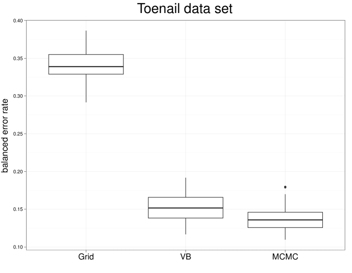
Figure 2: Toenail data set. Balanced error rate for grid search, random intercept VB and random intercept MCMC inference.

4.4 Variable selection

The example illustrates the use of a sparse prior for VB and MCMC inference on the spam data set (Frank and Asuncion, 2010). The spam data set was collected at the Hewlett-Packard Labs and consists of information from 4601 e-mails. A prediction vector of 57 variables was created for each e-mail and the goal is to predict whether the e-mail is spam or non-spam. The 57 variables include 54 percentages of word or character frequency in the e-mails and the 3 remaining predictors are related to the use of capital letters: the average length of uninterrupted sequences of capital letters, the length of the longest uninterrupted sequence of capital letters and the total number of capital letters in the e-mail. Note that all predictors are standardized prior to analysis.

The model we consider is similar to that used by Polson and Scott (2011) on the same data set with $\rho$ also fixed at 0.01. Appendix B summarizes the full conditionals for our MCMC scheme and we use a burn-in size of 50000 samples and a retained set of 50000 samples because of slower mixing.

Figure 3 illustrates the inclusion probabilities for each variable. Computing $P(v_{k}>0|\boldsymbol{y})$ enables to visualize the results as black bars for variables that are strongly associated with the presence of spam, while the opposite is true for white bars. Although VB generates more extreme inclusion probabilities there exists good agreement between the VB and MCMC results. The 24 variables that are almost certainly selected by MCMC match with the selected ones for VB, except for the variable cs. Variables that are selected by VB correspond to MCMC selected ones, although hpl and font have slightly lower probabilities for MCMC. The two VB selected variables with smallest inclusion probabilities, i.e., email and table also have lower MCMC inclusion probabilities. In terms of speed VB is favorable over MCMC taking 76 minutes compared to over 10 hours for MCMC.

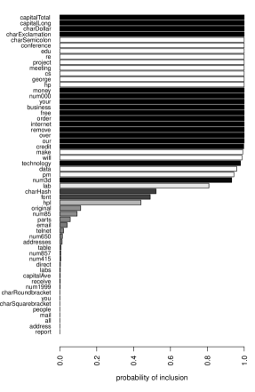
Figure 3: Spam data set. Inclusion probabilities for VB and MCMC inference with a Laplace-zero prior and $\rho=0.01$ in (a) and (b), respectively. The bars are shaded in proportion to $P(v_{k}>0|\boldsymbol{y})$, where darker means a greater probability for positive association with spam.

4.5 Missing predictor values

The final example represents a classification problem where the interest lies in predicting the presence of significant coronary disease, which is defined as 75% or more diameter narrowing in at least one important coronary artery. The data consist of measurements from 3504 patients who were referred to Duke University Medical Center for chest pain, and are available through the Duke University Cardiovascular Disease Databank (Harrell, 2001). For each patient we have the age, sex, duration of symptoms of coronary artery disease and the cholesterol level as predictors. The latter two variables are log-transformed and the variables are standardized prior to analysis so that all variables are approximately standard normal. Importantly, the variable cholesterol level has 1246 missing values.

The data set is repeatedly randomly split into a training and test part in such a way that all test cases have observed values for cholesterol level. For each split the BER on test set is computed for a traditional linear SVM and the missing predictor value VB (Algorithm 4) and MCMC (see Appendix C) approaches. Chapter 10 of Harrell (2001) presents a logistic regression analysis of this data set where only the complete cases were retained from the original set.

We compare our approaches against the default SVM approach which uses only complete cases for training. On the other hand, complete training cases and training cases with missing values for cholesterol level are used for the VB approach and the MCMC scheme. Figure 4 visualizes the boxplots of the BERs on test data for each of the three approaches.

These results illustrate that methodology which allows to include input vectors with missing values for training can yield better classification performance. In addition, the VB performance seems to be slightly better than the MCMC performance. Finally, the default SVM approach took on average 3109.40 seconds, the VB approach took 1028.18 seconds and the MCMC approach took 1718.98. Hence, even when missing data are present the VB approach is competitive both in terms of classification performance and computational efficiency.

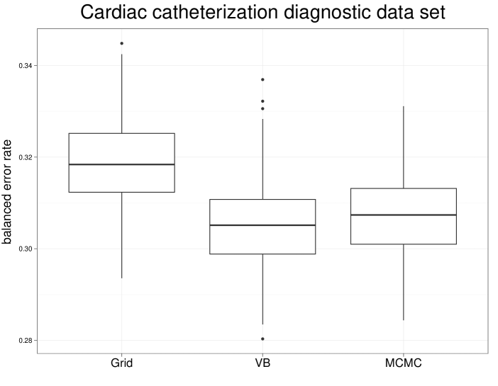
Figure 4: Cardiac catheterization diagnostic data set. Balanced error rate for grid search with complete training cases, VB and MCMC inference in the presence of missing predictor values.

5 Discussion

We have developed a VB approach to SVM classification. We have shown that the approach is a unified framework for dealing with a variety of complications typically difficult to deal with within a standard SVM framework. For the examples that we present here our VBSVM methods have as good or better classification performance than the standard SVM approach whilst remaining computationally efficient.

Appendix A – MCMC Scheme for Section 3.1

The full conditionals for MCMC inference are

$$\begin{array}[]{rl}\boldsymbol{\beta},\boldsymbol{u}|\mbox{rest}&\displaystyle\sim N\Bigg{\{}\left(\boldsymbol{C}^{T}\mbox{diag}(\boldsymbol{a}^{-1})\boldsymbol{C}+\mbox{blockdiag}(\sigma_{\beta}^{-2}\boldsymbol{I}_{p},\sigma_{u}^{-2}\boldsymbol{I}_{m})\right)^{-1}\boldsymbol{C}^{T}\boldsymbol{Y}(\boldsymbol{1}_{n}+\boldsymbol{a}^{-1}),\\ &\displaystyle\qquad\qquad\left(\boldsymbol{C}^{T}\mbox{diag}(\boldsymbol{a}^{-1})\boldsymbol{C}+\mbox{blockdiag}(\sigma_{\beta}^{-2}{\bf I}_{p},\sigma_{u}^{-2}\boldsymbol{I}_{m})\right)^{-1}\Bigg{\}},\\ \sigma_{u}^{2}|\mbox{rest}&\sim\mbox{IG}\left(A_{u}+\tfrac{m}{2},B_{u}+\tfrac{1}{2}\|\boldsymbol{u}\|^{2}\right),\\ a_{i}|\mbox{rest}&\sim\mbox{GIG}\left(\tfrac{1}{2},1,(1-y_{i}(\boldsymbol{x}_{i}^{T}\boldsymbol{\beta}+\boldsymbol{z}^{T}_{i}\boldsymbol{u}))^{2}\right),\end{array}$$

where $y_{i}$ is the $i$th element of ${\bf y}$ and ${\bf x}_{i}$ and ${\bf z}_{i}$ are the $i$th row of the matrices ${\bf X}$ and ${\bf Z}$ respectively. These can be used to implement a Gibbs sampling MCMC method.

Appendix B – MCMC Scheme for Section 3.2

The full conditionals for MCMC inference are

$$\begin{array}[]{rl}\boldsymbol{\beta},\boldsymbol{v}|\mbox{rest}&\sim N\Big{\{}\left(\widetilde{\boldsymbol{\Gamma}}\boldsymbol{C}^{T}\mbox{diag}(\boldsymbol{a}^{-1})\boldsymbol{C}\widetilde{\boldsymbol{\Gamma}}+\mbox{blockdiag}(\sigma_{\beta}^{-2}{\bf I}_{p},\sigma_{u}^{-2}\mbox{diag}(\boldsymbol{b}))\right)^{-1}\widetilde{\boldsymbol{\Gamma}}\boldsymbol{C}^{T}\boldsymbol{Y}(\boldsymbol{1}_{n}+\boldsymbol{a}^{-1}),\\ &\displaystyle\qquad\left(\widetilde{\boldsymbol{\Gamma}}\boldsymbol{C}^{T}\mbox{diag}(\boldsymbol{a}^{-1})\boldsymbol{C}\widetilde{\boldsymbol{\Gamma}}+\mbox{blockdiag}(\sigma_{\beta}^{-2}{\bf I}_{p},\sigma_{u}^{-2}\mbox{diag}(\boldsymbol{b}))\right)^{-1}\Big{\}},\\ \sigma_{u}^{2}|\mbox{rest}&\sim\mbox{IG}\left(A_{u}+\tfrac{m}{2},B_{u}+\tfrac{1}{2}\boldsymbol{v}^{T}\mbox{diag}(\boldsymbol{b})\boldsymbol{v}\right),\\ a_{i}|\mbox{rest}&\sim\mbox{GIG}(\tfrac{1}{2},1,(1-y_{i}(\boldsymbol{x}_{i}^{T}\boldsymbol{\beta}+\boldsymbol{z}_{i}^{T}\boldsymbol{\Gamma}\boldsymbol{v}))^{2}),\\ b_{k}|\mbox{rest}&\sim\mbox{Inverse-Gaussian}(\sigma_{u}/|v_{k}|,1),\\ \gamma_{k}|\mbox{rest}&\sim\mbox{Bernoulli}\Big{[}\mbox{expit}\Big{\{}\mbox{logit}(\rho)-\tfrac{1}{2}\boldsymbol{Z}^{T}_{k}\mbox{diag}(\boldsymbol{a}^{-1})\boldsymbol{Z}_{k}v_{k}^{2}+v_{k}\boldsymbol{Z}^{T}_{k}\mbox{diag}(\boldsymbol{1}_{n}+\boldsymbol{a}^{-1})\boldsymbol{y}\\ &\qquad\qquad-v_{k}\boldsymbol{Z}^{T}_{k}\mbox{diag}(\boldsymbol{a}^{-1})(\boldsymbol{X}\boldsymbol{\beta}+\boldsymbol{Z}_{-k}\mbox{diag}(\boldsymbol{\gamma}_{-k})\boldsymbol{v}_{-k})\Big{\}}\Big{]},\end{array}$$

where $\widetilde{\boldsymbol{\gamma}}=[\boldsymbol{1}^{T}_{p},\boldsymbol{\gamma}^{T}]^{T}$ and $\widetilde{\boldsymbol{\Gamma}}=\mbox{diag}(\widetilde{\boldsymbol{\gamma}})$.

Appendix C – MCMC Scheme for Section 3.3

The full conditionals for MCMC inference are

$$\begin{array}[]{rl}\beta,\boldsymbol{u}|\mbox{rest}&\sim N\Big{\{}\left(\boldsymbol{C}^{T}\mbox{diag}(\boldsymbol{a}^{-1})\boldsymbol{C}+\mbox{blockdiag}(\sigma_{\beta}^{-2},\sigma_{u}^{-2}\boldsymbol{I}_{d})\right)^{-1}\boldsymbol{C}^{T}\boldsymbol{Y}(\boldsymbol{1}_{n}+\boldsymbol{a}^{-1}),\\ &\displaystyle\qquad\qquad\left(\boldsymbol{C}^{T}\mbox{diag}(\boldsymbol{a}^{-1})\boldsymbol{C}+\mbox{blockdiag}(\sigma_{\beta}^{-2},\sigma_{u}^{-2}\boldsymbol{I}_{p})\right)^{-1}\Big{\}},\\ \sigma_{u}^{2}|\mbox{rest}&\sim\mbox{IG}\left(A_{u}+\tfrac{d}{2},B_{u}+\tfrac{1}{2}\|\boldsymbol{u}\|^{2}\right),\\ a_{i}|\mbox{rest}&\sim\mbox{GIG}\left(\tfrac{1}{2},1,(1-y_{i}(\beta+{\bf d}_{i}^{T}\boldsymbol{u}))^{2}\right),\\ \boldsymbol{\mu}|\mbox{rest}&\sim N\left[\left\{n\boldsymbol{\Sigma}^{-1}+\sigma_{\mu}^{-2}\boldsymbol{I}_{d}\right\}^{-1}n\boldsymbol{\Sigma}^{-1}\overline{{\bf d}},\left\{n\boldsymbol{\Sigma}^{-1}+\sigma_{\mu}^{-2}\boldsymbol{I}_{p}\right\}^{-1}\right],\\ \boldsymbol{\Sigma}|\mbox{rest}&\sim\mbox{IW}\left(\boldsymbol{\Psi}+\boldsymbol{D}^{T}\boldsymbol{D}-2n\overline{{\bf d}}\boldsymbol{\mu}^{T}+n\boldsymbol{\mu}\boldsymbol{\mu}^{T},\nu+n\right),\\ {\bf d}_{i,\mathcal{M}_{i}}|\mbox{rest}&\sim N\Big{[}\left\{\boldsymbol{P}_{i}^{T}\left[\boldsymbol{\Sigma}^{-1}+a_{i}^{-1}\boldsymbol{u}\boldsymbol{u}^{T}\right]\boldsymbol{P}_{i}\right\}^{-1}\par\boldsymbol{P}_{i}^{T}\Big{[}\boldsymbol{\Sigma}^{-1}\boldsymbol{\mu}+y_{i}(1+a_{i}^{-1})\boldsymbol{u}-a_{i}^{-1}\beta\boldsymbol{u}\\ &\qquad\qquad-\left[\boldsymbol{\Sigma}^{-1}+a_{i}^{-1}\boldsymbol{u}\boldsymbol{u}^{T}\right]\boldsymbol{Q}_{i}\boldsymbol{Q}_{i}^{T}{\bf d}_{i}\Big{]},\par\left\{\boldsymbol{P}_{i}^{T}\left[\boldsymbol{\Sigma}^{-1}+a_{i}^{-1}\boldsymbol{u}\boldsymbol{u}^{T}\right]\boldsymbol{P}_{i}\right\}^{-1}\Big{]},\end{array}$$

with $\overline{{\bf d}}=\frac{1}{n}\sum_{i=1}^{n}{\bf d}_{i}.$

References

• Andrews and Mallows (1974) Andrews, D. F., Mallows, C. L., 1974. Scale mixtures of normal distributions. Journal of the Royal Statistical Society, Series B 36, 99–102.
• Bernardo (1979) Bernardo, J. M., 1979. Expected information as expected utility. The Annals of Statistics 7, 686–690.
• Bishop (2006) Bishop, C. M., 2006. Pattern Recognition and Machine Learning. Springer, New York.
• Bishop and Tipping (2000) Bishop, C. M., Tipping, M. E., 2000. Variational relevance vector machines. In: Proceedings of the 16th Conference on Uncertainty in Artificial Intelligence. Stanford, pp. 46–53.
• Boser et al. (1992) Boser, B. E., Guyon, I. M., Vapnik, V. N., 1992. A training algorithm for optimal margin classifiers. In: Proceedings of the Annual Workshop on Computational Learning Theory. Pittsburgh, pp. 144–152.
• Chu et al. (2006) Chu, W., Keerthi, S. S., Ong, C. J., Ghahramani, Z., 2006. Bayesian support vector machines for feature ranking and selection. In: Guyon, I., Gunn, S., Nikravesh, M., Zadeh, L. (Eds.), Feature Extraction, Foundations and Applications. Springer, London, pp. 403–418.
• Cristianini and Shawe-Taylor (2000) Cristianini, N., Shawe-Taylor, J., 2000. An Introduction to Support Vector Machines and Other Kernel-Based Learning Methods. Cambridge University Press, New York.
• De Backer et al. (1998) De Backer, M., De Vroey, C., Lesaffre, E., Scheys, I., De Keyser, P., 1998. Twelve weeks of continuous oral therapy for toenail onychomycosis caused by dermatophytes: A double-blind comparative trial of Terbinafine 250 mg/day versus Itraconazole 200 mg/day. Journal of the American Academy of Dermatology 38, S57–S63.
• Dundar et al. (2007) Dundar, M., Krishnapuram, B., Bi, J., Rao, R. B., 2007. Learning classifiers when the training data is not IID. In: Proceedings of the 20th International Joint Conference on Artifical Intelligence. Hyderabad, pp. 756–761.
• Faes et al. (2011) Faes, C., Ormerod, J. T., Wand, M. P., 2011. Variational Bayesian inference for parametric and nonparametric regression with missing data. Journal of the American Statistical Association 106, 959–971.
• Frank and Asuncion (2010) Frank, A., Asuncion, A., 2010. UCI machine learning repository.
URL http://archive.ics.uci.edu/ml
• Gao and Wong (2005) Gao, Z., Wong, K. Y. M., 2005. Variational bayesian approach to support vector regression. Progress of Theoretical Physics Supplement 157, 284–287.
• Gold et al. (2005) Gold, C., Holub, A., Sollich, P., 2005. Bayesian approach to feature selection and parameter tuning for support vector machine classifiers. Neural Networks 18, 693–701.
• Guyon et al. (2002) Guyon, I., Weston, J., Barnhill, S., Vapnik, V. N., 2002. Gene selection for cancer classification using support vector machines. Machine Learning 46, 389–422.
• Harrell (2001) Harrell, F. E., 2001. Regression Modeling Strategies: with Applications to Linear Models, Logistic Regression and Survival Analysis. Springer-Verlag, New York.
• Hastie et al. (2009) Hastie, T. R., Tibshirani, R., Friedman, J., 2009. The Elements of Statistical Learning, 2nd Edition. Springer, New York.
• Kim (2009) Kim, J. H., 2009. Estimating classification error rate: Repeated cross-validation, repeated holdout and bootstrap. Computational Statistics and Data Analysis 53, 3735–3745.
• Lu et al. (2011) Lu, Z., Leen, T. K., Kaye, J., 2011. Kernels for longitudinal data with variable sequence length and sampling intervals. Neural Computation 23, 2390–2420.
• Luts et al. (2012) Luts, J., Molenberghs, G., Verbeke, G., Van Huffel, S., Suykens, J. A. K., 2012. A mixed effects least squares support vector machine model for classification of longitudinal data. Computational Statistics & Data Analysis 56, 611–628.
• Mallick et al. (2005) Mallick, B. K., Ghosh, D., Ghosh, M., 2005. Bayesian classification of tumours by using gene expression data. Journal of the Royal Statistical Society, Series B 67, 219–234.
• Nebot-Troyano and Belanche-Muñoz (2010) Nebot-Troyano, G., Belanche-Muñoz, L. A., 2010. A kernel extension to handle missing data. In: Bramer, M., Ellis, R., Petridis, M. (Eds.), Research and Development in Intelligent Systems XXVI. Springer, London, pp. 165–178.
• Ormerod and Wand (2010) Ormerod, J. T., Wand, M. P., 2010. Explaining variational approximations. The American Statistician 64, 140–153.
• Pearce and Wand (2009) Pearce, N. D., Wand, M. P., 2009. Explicit connections between longitudinal data analysis and kernel machines. Electronic Journal of Statistics 3, 797–823.
• Pelckmans et al. (2005) Pelckmans, K., De Brabanter, J., Suykens, J. A. K., De Moor, B., 2005. Handling missing values in support vector machine classifiers. Neural Networks 18, 684–692.
• Polson and Scott (2011) Polson, N. G., Scott, S. L., 2011. Data augmentation for support vector machines. Bayesian Analysis 6, 1–23.
• Ruppert et al. (2003) Ruppert, D., Wand, M. P., Carroll, R. J., 2003. Semiparametric Regression. Cambridge University Press, New York.
• Smola et al. (2005) Smola, A. J., Vishwanathan, S. V. N., Hofmann, T., 2005. Kernel methods for missing variables. In: Proceedings of the Tenth International Workshop on Artificial Intelligence and Statistics. Barbados, pp. 325–332.
• Tipping (2001) Tipping, M. E., 2001. Sparse Bayesian learning and the relevance vector machine. Journal of Machine Learning Research 1, 211–244.
• Vapnik (1998) Vapnik, V. N., 1998. Statistical Learning Theory. Wiley, New York.
• Wand (2003) Wand, M. P., 2003. Smoothing and mixed models. Computational Statistics 18, 223–249.
• Wand and Ormerod (2008) Wand, M. P., Ormerod, J. T., 2008. On semiparametric regression with O’Sullivan penalised splines. Australian and New Zealand Journal of Statistics 50, 179–198.
• Wand and Ormerod (2011) Wand, M. P., Ormerod, J. T., 2011. Penalized wavelets: Embedding wavelets into semiparametric regression. Electronic Journal of Statistics 5, 1654–1717.
• Weston et al. (2000) Weston, J., Mukherjee, S., Chapelle, O., Pontil, M., Poggio, T., Vapnik, V., 2000. Feature selection for SVMs. In: Proceedings of the Annual Conference on Neural Information Processing Systems 13. Denver, pp. 668–674.
• Zhang et al. (2011) Zhang, D., Dai, G., Jordan, M. I., 2011. Bayesian generalized kernel mixed models. Journal of Machine Learning Research 12, 111–139.
• Zhao et al. (2006) Zhao, Y., Staudenmayer, J., Coull, B. A., Wand, M. P., 2006. General design Bayesian generalized linear mixed models. Statistical Science 21, 35–51.
• Zhu et al. (2003) Zhu, J., Rosset, S., Hastie, T., Tibshirani, R., 2003. 1-norm support vector machines. In: Proceedings of the Annual Conference on Neural Information Processing Systems 16. Vancouver.