Effects of Density Conservation and Hydrodynamics on Aging in Nonequilibrium Processes
Abstract
Aging in kinetics of three different phase transitions, viz., magnetic, binary solid and single component fluid, have been studied via Monte Carlo and molecular dynamics simulations in three space dimensions with the objective of identifying the effects of order-parameter conservation and hydrodynamics. We observe that the relevant autocorrelations exhibit power-law decay in ferromagnet and binary solid but with different exponents. At early time fluid autocorrelation function nicely follows that of binary solid, the order parameter being conserved for both of them, as opposed to a ferromagnet. At late time the fluid data crosses over to an exponential decay which we identify as a hydrodynamic effect and provide analytical justification for this behavior.
pacs:
81.40.Cd, 72.15.CzUnderstanding properties related to aging Zannetti in out of equilibrium systems is of fundamental as well as of practical importance. Systems of interest are in abundance Mathieu ; Abou ; Costa ; Kenning ; Berthier ; Masri ; Bouchbinder ; Bergli , starting from biology to cosmology. In the literature of nonequilibrium statistical mechanics, even though the quantities involving single time are reasonably well understood Bray , those involving multiple time remained difficult. Aging phenomena is related to the latter where one expects slower relaxation of older systems. Apart from this obvious qualitative fact, understanding of this important phenomena is very poor even for simplest of the systems.
In this letter, we present results from the studies of aging kinetics in nonequilibrium systems following three distinctly different phase transitions with the objective to understand the effects of order-parameter conservation and hydrodynamics on this phenomena. For this purpose we have studied the two-time or autocorrelation function Zannetti , , defined as
| (1) |
where is the relevant space () and time () dependent order parameter. In Eq. (1), and are referred to as the observation and waiting times, respectively – the latter essentially is the age of the system.
Fisher and Huse (FH) DFisher , from the study of spin glass systems, predicted a power-law decay of , in space dimensions, as
| (2) |
where and are characteristic lengths of a system at time and , respectively. However, not much further information have been obtained either on the value of the exponent or on the general validity of a power-law decay, particularly for systems with conserved order-parameter dynamics.
In this work, from the comparative studies of aging dynamics in systems undergoing ferromagnetic ordering, phase separation in a solid binary mixture and that in a vapor-liquid system, we obtain significant general understanding. Note that having been quenched from a homogeneous state to a temperature () below the critical one (), these systems move towards the new equilibrium state via formation and growth of domains as Bray
| (3) |
In case of a ferromagnet, where one has nonconserved order-parameter, the exponent has a value Bray ; for phase separating binary solid, for which the order-parameter is a conserved quantity Bray ; LS ; Suman_Ising , . In fluids, however, the entire growth process cannot be described by a single exponent. This complexity is due to the influence of hydrodynamics Siggia ; Furukawa ; Suman_VL ; Shaista . In this case the early time growth is consistent with the binary solid due to diffusive transport. At late time, the exponent crosses over to , referred to as the viscous hydrodynamic regime and further to the inertial hydrodynamic regime with . It is crucial to understand the effects of and thus the growth mechanism, on the decay of .
To address these issues, we have considered two different models. For the growth dynamics in ferromagnet and solid binary mixture, we have studied the nearest neighbor Ising model prototype for a variety of phase transitions. For a binary (A+B) mixture spin value corresponds to an A-particle and to a B-particle. The kinetics in this model was studied via Monte Carlo (MC) simulations MCbook . In the nonconserved case we have implemented the Glauber spin-flip kinetics MCbook where in a trial MC move the sign of a randomly chosen spin was altered and the move was accepted or rejected according to standard Metropolis criterion. In case of conserved kinetics, we have used the Kawasaki exchange mechanism MCbook where, in a trial move, positions of a randomly chosen nearest neighbor pair of spins were interchanged. On the other hand, for the vapor-liquid transition, we have carried out molecular dynamics (MD) simulations Frenkel on a model where particles of equal mass () interact with each other via Suman_VL where is the standard Lennard-Jones (LJ) potential, with and being respectively the interaction strength and particle diameter. Here the cut-off distance was introduced for faster computation.

As opposed to the MC simulation of Ising model where the spins or particles sit only on sites of a regular lattice system (of lattice constant ), in the MD simulations particles can change their positions continuously. To control the temperature in MD simulations, we have used the Nosé-Hoover thermostat Frenkel that preserves hydrodynamics well. For the Ising model, time was measured in units of the Monte Carlo Steps (MCS) with one MCS consisting of trial moves, being the linear dimension of the system. For the MD runs, we have the LJ time unit . In the rest of the paper, we set , , , , and the Boltzmann constant to unity. Then the LJ unit becomes unity as well.
In addition to , , that will often be used, was obtained from the first moment of the domain size distribution function as where is the distance between two successive domain boundaries in , , or directions. All our results are obtained with periodic boundary conditions. For the Ising model we have chosen a simple cubic lattice. For the analysis of LJ system results, the continuous original configurations were mapped to a simple cubic lattice Suman_VL . In this procedure, every particle was moved to the nearest lattice site, following which if a site is occupied by a particle it was assigned a spin value , otherwise . Note that in Eq. (1) corresponds to these spin values. Quantitative results are presented after averaging over multiple initial configurations. Before presenting the results, we mention that for the Ising model MCbook and for the LJ system it is Sutapa . In all the cases, quenching was done along the critical composition or density (). For Ising model, of course, this corresponds to a composition of up and down spins, while for the LJ model we have Suman_VL ; Sutapa .
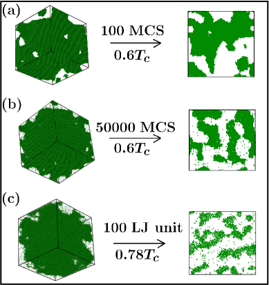
In Fig. 1, we show snapshots from the evolutions of all three systems, starting from homogeneous initial configurations. The temperatures of quench in each of the cases are mentioned on the figure. The frames on the left are original configurations. For better judgement of the pattern, on the right hand side frames we show slices of the systems. It appears that there is significant difference in morphology for the conserved and nonconserved dynamics Bray . Also, if the dynamics is conserved, effect of hydrodynamics does not, at least, bring visibly different features in the pattern as is clear from the snapshots from binary solid and vapor-liquid systems.

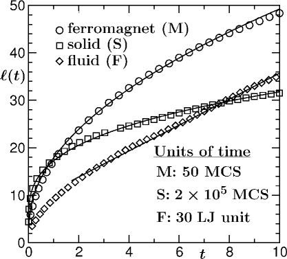
The growth dynamics is compared, for all the systems, in Fig. 2 where we plot as a function of . The continuous lines in this figure are fits to the expected theoretical exponents. For the Ising model, it is clearly seen that the data are consistent with exponents and for the conserved and nonconserved dynamics respectively. For the LJ model, however, after a brief period of slow growth, there is a crossover to a regime where the simulation data are nicely consistent with a linear behavior corresponding to viscous hydrodynamic growth Suman_VL . We do not aim for a further crossover to the inertial hydrodynamic regime due to lack of computational resources. Next we move to the central objective of the paper.
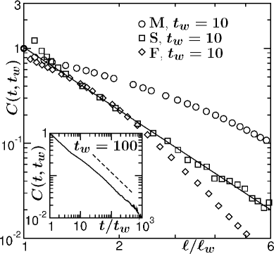
In Fig. 3 we show the plots of vs for all the systems. A double-log scale is used and the values of in each of the cases are mentioned on the figure. It is seen that the data for the solid binary mixture is consistent with a power-law decay starting from very small value of the abscissa variable till the end of the available simulation results. The continuous line there has an exponent with which this set of data are nicely consistent. The results for ferromagnet or vapor-liquid system does not show linear look over the whole range. However, the fluid data are consistent with the solid mixture result at the beginning. This is due to the fact that hydrodynamics becomes important only at large length scales as already seen in Fig. 2. Around the value of from where we have seen a linear behavior for the LJ system in Fig. 2, we observe a deviation from the power-law in this figure. One can also ask, if the continuous curvature of the ferromagnetic data is also indicative of a non-power-law decay? Before moving on to answer these questions, in the inset of Fig. 3 we show vs for the binary solid only. Again the data look very linear, after a brief initial period, on a double log scale and are consistent with a power-law exponent . This indirectly confirms that for diffusive kinetics with conserved order parameter is with which, of course, early time fluid results are consistent. The value is, of course, consistent with the bound predicted by FH DFisher ; Marko . However, this is in disagreement with similar studies Desai via Cahn Hilliard equation Bray .

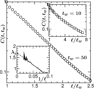
Next, in the main frame of Fig. 4 we show log-linear plots of vs for the vapor-liquid transition. Note here that we have chosen a value of such that the system is in the hydrodynamic regime. The minimum value of needed for this can be read out from Fig. 2. This data clearly looks linear on this plot which confirms exponential decay of the autocorrelation function. The ferromagnet data, presented in the upper inset of Fig. 4, however, is inconsistent with it. Note here that in all the cases we have experimented with various values of for general understanding of scaling with respect to or and for the sake of brevity presented only the representative ones.
In view of the other expectation that the ferromagnetic data follow a power-law behavior with time or length dependent correction, in the lower inset of Fig. 4 we present the instantaneous exponent Huse as a function of . It appears that has a linear dependence on , for a significant period of time. The minor deviation at late time, we confirmed, is a finite-size effect. If we neglect the part affected by finite-size effects, the data converge to a value , predicted by theoretical calculations of Liu and Mazenko Liu . Thus there is no universality involving conserved and nonconserved dynamics, even though in both cases follow power-law decay.

Finally, we come to the understanding of the exponential decay, that was also recently observed in liquid-liquid transition Lippiello , for the vapor-liquid transition in the hydrodynamic regime. To accomplish that we start with the order-parameter update equation of model H Bray
| (4) |
where is the advection field, is a diffusion constant and is the chemical potential. With the understanding that in the fast hydrodynamic regime, contribution from diffusion is negligible, we neglect the term on the right hand side. From the definition of the autocorrelation function in Eq. (1), it is clear that our task is to show that the order-parameter changes exponentially fast. Here we make an assumption that this exponential decay is due to fast interfacial motion. Noting that for the viscous hydrodynamic growth, is constant () and in the interfacial region , being the interfacial width, we obtain where is a constant. This provides .
In conclusion, we have presented results for aging during the nonequilibrium evolutions in various systems – ferromagnet, solid binary mixture and vapor-liquid system – following quench from high temperatures below the critical ones. The two-time correlation function Zannetti has been used as a probe for this study. The Ising model with conserved and nonconserved order-parameter dynamics were used to study the binary solid and ferromagnetic systems, respectively, while an LJ model Suman_VL was used for the study of fluid.
It is observed that in absence of hydrodynamics, in all the cases the autocorrelation decays in a power-law fashion. The exponent for the conserved order-parameter dynamics deviates significantly from the nonconserved one, but both of them follow the bounds predicted by Fisher and Huse DFisher . Interestingly, for the nonconserved case, there is significant curvature dependent correction to the exponent. At late time, in fluid, there is a crossover from power-law to an exponential behavior which we understood via analytical argument.
Acknowledgment
SKD acknowledges important discussion with M. Zannetti, S. Puri, F. Corberi and E. Lippiello. Both of us acknowledge financial support from the Department of Science and Technology, India, via grant no. SR/S2/RJN-13/2009. SM is grateful to Council of Scientific and Industrial Research, India, for research fellowship.
das@jncasr.ac.in
References
- (1) M. Zannetti in Kinetics of Phase Transitions, edited by S. Puri and V. Wadhawan (2009).
- (2) R. Mathieu, P. Norblad, D.N.H. Nam, N.X. Phue and N.V. Khiem, Phys. Rev. B 63, 174405 (2001).
- (3) B. Abou and F. Gallet, Phys. Rev. Lett. 93, 160603 (2004).
- (4) M. Costa, A.L. Goldberger and C.-K. Peng, Phys. Rev. Lett. 95, 198102 (2005).
- (5) G.G. Kenning, G.F. Rodriguez and R. Orbach, Phys. Rev. Lett. 97, 057201 (2006).
- (6) L. Berthier, Phys. Rev. Lett. 98, 220601 (2007).
- (7) D.E. Masri, L. Berthier and L. Cipelletti, Phys. Rev. E 82, 031503 (2007).
- (8) E. Bouchbinder and J.S. Langer, Phys. Rev. E 83, 061503 (20011).
- (9) J. Bergli and Y.M. Galperin, Phys. Rev. B 85, 214202 (20012).
- (10) A.J. Bray, Adv. Phys. 51, 481 (2002).
- (11) D.S. Fisher and D.A. Huse, Phys. Rev. B, 38, 373 (1989).
- (12) I.M. Lifshitz and V.V. Slyozov, J. Phys. Chem. Solids 19, 35 (1961).
- (13) S. Majumder and S.K. Das, Phys. Rev. E 81, 050102 (2010).
- (14) E.D. Siggia, Phys. Rev. A 20, 595 (1979).
- (15) H. Furukawa, Phys. Rev. A 31, 1103 (1985).
- (16) S. Majumder and S.K. Das, Europhys. Lett. 95, 46002 (2011).
- (17) S. Ahmad, S.K. Das and S. Puri, Phys. Rev. E 82, 040107 (2010).
- (18) D.P. Landau and K. Binder, A Guide to Monte Carlo Simulations in Statistical Physics, Cambridge University Press, 3rd Edition (2009).
- (19) D. Frenkel and B. Smit, Understanding Molecular Simulations: From Algorithm to Applications (Academic Press, San Diego, 2002).
- (20) S. Roy and S.K. Das, Phys. Rev. E 85, 050602 (2012).
- (21) J.F. Marko and G.T. Barkema, Phys. Rev. E 52, 2522 (1995).
- (22) C. Yeung, M. Rao and R.C. Desai, Phys. Rev. E 53, 3073 (1996).
- (23) D.A. Huse, Phys. Rev. B, 40, 304 (1989).
- (24) F. Liu and G.F. Mazenko, Phys. Rev. B 44, 9185 (1991).
- (25) S. Ahmad, F. Corberi, S.K. Das, E. Lippiello, S. Puri and M. Zannetti, Phys. Rev. E 86, 061129 (2012).