Weight Distribution for Non-binary Cluster LDPC Code Ensemble

Takayuki Nozaki Kanagawa University, JAPAN
Email: nozaki@kanagawa-u.ac.jp
   Masaki Maehara, Kenta Kasai, and Kohichi Sakaniwa Tokyo Institute of Technology, JAPAN
Email: {maehara, kenta, sakaniwa}@comm.ce.titech.ac.jp
Abstract

In this paper, we derive the average weight distributions for the irregular non-binary cluster low-density parity-check (LDPC) code ensembles. Moreover, we give the exponential growth rate of the average weight distribution in the limit of large code length. We show that there exist (2,dc2subscript𝑑c2,d_{\mathrm{c}})-regular non-binary cluster LDPC code ensembles whose normalized typical minimum distances are strictly positive.

I Introduction

Gallager invented low-density parity-check (LDPC) codes [1]. Due to the sparseness of the parity check matrices, LDPC codes are efficiently decoded by the belief propagation (BP) decoder. Optimized LDPC codes can exhibit performance very close to the Shannon limit [2]. Davey and MacKay [3] have found that non-binary LDPC codes can outperform binary ones.

The LDPC codes are defined by sparse parity check matrices or sparse Tanner graphs. For the non-binary LDPC codes, the Tanner graphs are represented by bipartite graph with variable nodes and check nodes and labeled edges. The LDPC codes defined by Tanner graphs with the variable nodes of degree dvsubscript𝑑vd_{\mathrm{v}} and the check nodes of degree dcsubscript𝑑cd_{\mathrm{c}} are called (dv,dc)subscript𝑑vsubscript𝑑c(d_{\mathrm{v}},d_{\mathrm{c}})-regular LDPC codes. It is empirically known that (2,dc)2subscript𝑑c(2,d_{\mathrm{c}})-regular non-binary LDPC codes exhibit good decoding performance among other LDPC codes for the non-binary LDPC code defined over Galois field of order greater than 323232 [4].

Savin and Declercq proposed the non-binary cluster LDPC codes [5]. For the non-binary cluster LDPC code, each edge in the Tanner graphs is labeled by cluster which is a full-rank p×r𝑝𝑟p\times r binary matrix, where pr𝑝𝑟p\geq r. In [5], Savin and Declercq showed that there exist (2,dc)2subscript𝑑c(2,d_{\mathrm{c}})-regular non-binary cluster LDPC ensembles whose minimum distance grows linearly with the code length.

Deriving the weight distribution is important to analyze the decoding performances for the linear codes. In particular, in the case for LDPC codes, weight distribution gives a bound of decoding error probability under maximum likelihood decoding [6] and error floors under belief propagation decoding and maximum likelihood decoding [7] [8].

Studies on weight distribution for non-binary LDPC codes date back to [1]. Gallager derived the symbol-weight distribution of Gallager code ensemble defined over /q𝑞\mathbb{Z}/q\mathbb{Z} [1]. Kasai et al. derived the average symbol and bit weight distributions and the exponential growth rates for the irregular non-binary LDPC code ensembles defined over Galois field 𝔽qsubscript𝔽𝑞\mathbb{F}_{q}, and showed that the normalized typical minimum distance does not monotonically grow with q𝑞q [9]. Andriyanova et al. derive the bit weight distributions and the exponential growth rates for the regular non-binary LDPC code ensembles defined over Galois field and general linear groups [10].

In this paper, we derive the average symbol and bit weight distributions for the irregular non-binary cluster LDPC code ensembles. Moreover, we give the exponential growth rate of the average weight distributions in the limit of large code length.

The remainder of this paper is organized as follows: Section II defines the irregular non-binary cluster LDPC code ensemble. Section III derives the average weight distributions for the irregular non-binary LDPC code ensembles. Section IV gives the exponential growth rate of the average weight distributions in the limit of large code length and shows some numerical examples for the exponential growth rate.

II Preliminaries

In this section, we review non-binary cluster LDPC code [5] and define the irregular non-binary cluster LDPC code ensemble. We introduce some notations used throughout this paper.

II-A Non-binary Cluster LDPC Code

The LDPC codes are defined by sparse parity check matrices or sparse Tanner graphs. For the non-binary LDPC codes, the Tanner graphs are represented by bipartite graphs with variable nodes and check nodes and labeled edges.

For the non-binary cluster LDPC codes, each edge in the Tanner graphs is labeled by cluster which is a full-rank p×r𝑝𝑟p\times r binary matrix, where pr𝑝𝑟p\geq r. Let 𝔽2subscript𝔽2\mathbb{F}_{2} be the finite field of order 2. Note that the non-binary LDPC codes defined by Tanner graphs labeled by general linear group GL(p,𝔽2)GL𝑝subscript𝔽2\mathrm{GL}(p,\mathbb{F}_{2}) are special cases for the non-binary cluster LDPC code with p=r𝑝𝑟p=r.

We denote the cluster in the edge between the i𝑖i-th variable node and the j𝑗j-th check node, by hj,isubscript𝑗𝑖h_{j,i}. For the cluster LDPC codes, r𝑟r-bits are assigned to each variable node in the Tanner graphs. We refer to the r𝑟r-bits assigned to the i𝑖i-th variable node as symbol assigned to the i𝑖i-th variable node, and denote it by 𝒙i𝔽2rsubscript𝒙𝑖superscriptsubscript𝔽2𝑟{\bm{x}}_{i}\in\mathbb{F}_{2}^{r}.

For integers a,b𝑎𝑏a,b, we denote the set of integers between a𝑎a and b𝑏b, as [a;b]𝑎𝑏[a;b]. More precisely, we define

[a;b]:={{nanb},ab,={},a>b.assign𝑎𝑏casesconditional-set𝑛𝑎𝑛𝑏𝑎𝑏𝑎𝑏\displaystyle[a;b]:=\begin{cases}\{n\in\mathbb{N}\mid a\leq n\leq b\},&a\leq b,\\ \emptyset=\{\},&a>b.\end{cases}

The non-binary cluster LDPC code defined by a Tanner graph 𝙶𝙶\mathtt{G} is given as follows:

C(𝙶)={(𝒙1,,𝒙N)(𝔽2r)Ni𝒩c(j)hj,i𝒙iT=𝟎T𝔽2pj[1;M]},𝐶𝙶conditional-setsubscript𝒙1subscript𝒙𝑁superscriptsuperscriptsubscript𝔽2𝑟𝑁subscript𝑖subscript𝒩c𝑗subscript𝑗𝑖superscriptsubscript𝒙𝑖𝑇superscript0𝑇superscriptsubscript𝔽2𝑝for-all𝑗1𝑀\displaystyle C(\mathtt{G})=\Bigl{\{}({\bm{x}}_{1},\dots,{\bm{x}}_{N})\in(\mathbb{F}_{2}^{r})^{N}\mid{\textstyle\sum_{i\in\mathcal{N}_{\mathrm{c}}(j)}}h_{j,i}{\bm{x}}_{i}^{T}={\bm{0}}^{T}\in\mathbb{F}_{2}^{p}~{}~{}\forall j\in[1;M]\Bigr{\}},

where 𝒩c(j)subscript𝒩c𝑗\mathcal{N}_{\mathrm{c}}(j) represents the set of indexes of the variable nodes adjacent to the j𝑗j-th check node. Note that N𝑁N is called symbol code length and the bit code length n𝑛n is given by rN𝑟𝑁rN.

II-B Irregular Non-binary Cluster LDPC Code Ensemble

Let \mathcal{L} and \mathcal{R} be the sets of degrees of the variable nodes and the check nodes, respectively. Irregular non-binary cluster LDPC codes are characterized with the number of variable nodes N𝑁N, the size of cluster p,r𝑝𝑟p,r and a pair of degree distribution, λ(x)=iλixi1𝜆𝑥subscript𝑖subscript𝜆𝑖superscript𝑥𝑖1\lambda(x)=\sum_{i\in{\cal L}}\lambda_{i}x^{i-1} and ρ(x)=iρixi1𝜌𝑥subscript𝑖subscript𝜌𝑖superscript𝑥𝑖1\rho(x)=\sum_{i\in{\cal R}}\rho_{i}x^{i-1}, where λisubscript𝜆𝑖\lambda_{i} and ρisubscript𝜌𝑖\rho_{i} are the fractions of the edges connected to the variable nodes and the check nodes of degree i𝑖i, respectively.

The total number of the edges in the Tanner graph is

E:=N01λ(x)dx.E:=\frac{N}{\int_{0}^{1}\lambda(x)dx.}

The number of check node M𝑀M is given by

M=(01ρ(x)𝑑x01λ(x)𝑑x)N=:κN.M=\biggl{(}\frac{\int_{0}^{1}\rho(x)dx}{\int_{0}^{1}\lambda(x)dx}\biggr{)}N=:\kappa N.

Let Lisubscript𝐿𝑖L_{i} and Rjsubscript𝑅𝑗R_{j} be the fraction of the variable nodes of degree i𝑖i and the check nodes of degree j𝑗j, respectively, i.e.,

Li:=λii01λ(x)𝑑x,Rj:=ρjj01ρ(x)𝑑x.formulae-sequenceassignsubscript𝐿𝑖subscript𝜆𝑖𝑖superscriptsubscript01𝜆𝑥differential-d𝑥assignsubscript𝑅𝑗subscript𝜌𝑗𝑗superscriptsubscript01𝜌𝑥differential-d𝑥\displaystyle L_{i}:=\frac{\lambda_{i}}{i\int_{0}^{1}\lambda(x)dx},\quad R_{j}:=\frac{\rho_{j}}{j\int_{0}^{1}\rho(x)dx}.

The design rate is given as follows:

1κpr.1𝜅𝑝𝑟1-\frac{\kappa p}{r}.

Assume that we are given the number of variable nodes N𝑁N, the size of cluster p,r𝑝𝑟p,r and the degree distribution pair (λ,ρ)𝜆𝜌(\lambda,\rho). An irregular non-binary cluster LDPC code ensemble 𝒢(N,p,r,λ,ρ)𝒢𝑁𝑝𝑟𝜆𝜌\mathcal{G}(N,p,r,\lambda,\rho) is defined as the following way. There exist LiNsubscript𝐿𝑖𝑁L_{i}N variable nodes of degree i𝑖i and RjMsubscript𝑅𝑗𝑀R_{j}M check nodes of degree j𝑗j. A node of degree i𝑖i has i𝑖i sockets for its connected edges. Consider a permutation π𝜋\pi on the number of edges. Join the i𝑖i-th socket on the variable node side to the π(i)𝜋𝑖\pi(i)-th socket on the check node side. The bipartite graphs are chosen with equal probability from all the permutations on the number of edges. Each cluster in an edge is chosen a full-rank p×r𝑝𝑟p\times r binary matrix with equal probability.

III Weight Distribution for Non-binary Cluster LDPC Code

In this section, we derive the average symbol and bit weight distribution for the irregular non-binary cluster LDPC code ensemble 𝒢(N,p,r,λ,ρ)𝒢𝑁𝑝𝑟𝜆𝜌\mathcal{G}(N,p,r,\lambda,\rho).

We denote the r𝑟r-bit representation of 𝒙i𝔽2rsubscript𝒙𝑖superscriptsubscript𝔽2𝑟{\bm{x}}_{i}\in\mathbb{F}_{2}^{r}, by (xi,1,,xi,r)subscript𝑥𝑖1subscript𝑥𝑖𝑟(x_{i,1},\dots,x_{i,r}). For a given codeword 𝒙=(𝒙1,𝒙2,,𝒙N)𝒙subscript𝒙1subscript𝒙2subscript𝒙𝑁{\bm{x}}=({\bm{x}}_{1},{\bm{x}}_{2},\dots,{\bm{x}}_{N}), we denote the symbol and bit weight of 𝒙𝒙{\bm{x}}, by w(𝒙)𝑤𝒙w({\bm{x}}) and wb(𝒙)subscript𝑤b𝒙w_{\mathrm{b}}({\bm{x}}). More precisely, we define

w(𝒙)𝑤𝒙\displaystyle w({\bm{x}}) :=|{i[1;N]𝒙i𝟎}|,assignabsentconditional-set𝑖1𝑁subscript𝒙𝑖0\displaystyle:=|\{i\in[1;N]\mid{\bm{x}}_{i}\neq{\bm{0}}\}|,
wb(𝒙)subscript𝑤b𝒙\displaystyle w_{\mathrm{b}}({\bm{x}}) :=|{(i,j)[1;N]×[1;r]xi,j0}|.assignabsentconditional-set𝑖𝑗1𝑁1𝑟subscript𝑥𝑖𝑗0\displaystyle:=|\{(i,j)\in[1;N]\times[1;r]\mid x_{i,j}\neq 0\}|.

For a given Tanner graph 𝙶𝙶\mathtt{G}, let A𝙶()superscript𝐴𝙶A^{\mathtt{G}}(\ell) (resp. Ab𝙶()subscriptsuperscript𝐴𝙶bA^{\mathtt{G}}_{\mathrm{b}}(\ell)) be the number of codeword of symbol and (resp. bit) weight \ell in C(𝙶)𝐶𝙶C(\mathtt{G}), i.e.,

A𝙶()=|{𝒙C(𝙶)w(𝒙)=}|,superscript𝐴𝙶conditional-set𝒙𝐶𝙶𝑤𝒙\displaystyle A^{\mathtt{G}}(\ell)=|\{{\bm{x}}\in C(\mathtt{G})\mid w({\bm{x}})=\ell\}|,
Ab𝙶()=|{𝒙C(𝙶)wb(𝒙)=}|.subscriptsuperscript𝐴𝙶bconditional-set𝒙𝐶𝙶subscript𝑤b𝒙\displaystyle A^{\mathtt{G}}_{\mathrm{b}}(\ell)=|\{{\bm{x}}\in C(\mathtt{G})\mid w_{\mathrm{b}}({\bm{x}})=\ell\}|.

For the irregular non-binary cluster LDPC code ensemble 𝒢(N,r,p,λ,ρ)𝒢𝑁𝑟𝑝𝜆𝜌\mathcal{G}(N,r,p,\lambda,\rho), we denote the average number of codewords of symbol and bit weight \ell, by A()𝐴A(\ell) and Ab()subscript𝐴bA_{\mathrm{b}}(\ell), respectively. Since each Tanner graph in the ensemble 𝒢=𝒢(N,r,p,λ,ρ)𝒢𝒢𝑁𝑟𝑝𝜆𝜌\mathcal{G}=\mathcal{G}(N,r,p,\lambda,\rho) is chosen with uniform probability, the following equations hold:

A()=1|𝒢|𝙶𝒢A𝙶(),Ab()=1|𝒢|𝙶𝒢Ab𝙶().formulae-sequence𝐴1𝒢subscript𝙶𝒢superscript𝐴𝙶subscript𝐴b1𝒢subscript𝙶𝒢subscriptsuperscript𝐴𝙶b\displaystyle A(\ell)=\frac{1}{|\mathcal{G}|}\sum_{\mathtt{G}\in\mathcal{G}}A^{\mathtt{G}}(\ell),\quad A_{\mathrm{b}}(\ell)=\frac{1}{|\mathcal{G}|}\sum_{\mathtt{G}\in\mathcal{G}}A^{\mathtt{G}}_{\mathrm{b}}(\ell).

Since the number of full-rank binary p×r𝑝𝑟p\times r matrix is i=0r1(2p2i)superscriptsubscriptproduct𝑖0𝑟1superscript2𝑝superscript2𝑖\prod_{i=0}^{r-1}(2^{p}-2^{i}), the number of codes in the ensemble 𝒢=𝒢(N,r,p,λ,ρ)𝒢𝒢𝑁𝑟𝑝𝜆𝜌\mathcal{G}=\mathcal{G}(N,r,p,\lambda,\rho) is given as

|𝒢|=E!{i=0r1(2p2i)}E.𝒢𝐸superscriptsuperscriptsubscriptproduct𝑖0𝑟1superscript2𝑝superscript2𝑖𝐸\displaystyle|\mathcal{G}|=E!\Biggl{\{}\prod_{i=0}^{r-1}(2^{p}-2^{i})\Biggr{\}}^{E}. (1)

III-A Symbol Codeword Weight Distribution

First, we will derive the average symbol weight distributions for the irregular non-binary cluster LDPC code ensembles.

Theorem 1

The average number A()𝐴A(\ell) of codewords of symbol weight \ell for the irregular non-binary cluster LDPC code ensemble 𝒢(N,p,r,λ,ρ)𝒢𝑁𝑝𝑟𝜆𝜌\mathcal{G}(N,p,r,\lambda,\rho) is

A()=k=0E(2r1)coef((P(s,t)Q(u))N,stkuk)(Ek)(2p1)k,𝐴superscriptsubscript𝑘0𝐸superscriptsuperscript2𝑟1coefsuperscript𝑃𝑠𝑡𝑄𝑢𝑁superscript𝑠superscript𝑡𝑘superscript𝑢𝑘binomial𝐸𝑘superscriptsuperscript2𝑝1𝑘\displaystyle A(\ell)=\sum_{k=0}^{E}\frac{(2^{r}-1)^{\ell}\mathrm{coef}\bigl{(}(P(s,t)Q(u))^{N},s^{\ell}t^{k}u^{k}\bigr{)}}{\binom{E}{k}(2^{p}-1)^{k}}, (2)
P(s,t):=i(1+sti)Li,Q(u):=jfj(u)κRj,formulae-sequenceassign𝑃𝑠𝑡subscriptproduct𝑖superscript1𝑠superscript𝑡𝑖subscript𝐿𝑖assign𝑄𝑢subscriptproduct𝑗subscript𝑓𝑗superscript𝑢𝜅subscript𝑅𝑗\displaystyle P(s,t):=\prod_{i\in\mathcal{L}}\bigl{(}1+st^{i}\bigr{)}^{L_{i}},\quad Q(u):=\prod_{j\in\mathcal{R}}f_{j}(u)^{\kappa R_{j}},
fj(u):=12p[{1+(2p1)u}j+(2p1)(1u)j],assignsubscript𝑓𝑗𝑢1superscript2𝑝delimited-[]superscript1superscript2𝑝1𝑢𝑗superscript2𝑝1superscript1𝑢𝑗\displaystyle f_{j}(u):=\frac{1}{2^{p}}\bigl{[}\{1+(2^{p}-1)u\}^{j}+(2^{p}-1)(1-u)^{j}\bigr{]}, (3)

where coef(g(s,t,u),sitjuk)coef𝑔𝑠𝑡𝑢superscript𝑠𝑖superscript𝑡𝑗superscript𝑢𝑘\mathrm{coef}(g(s,t,u),s^{i}t^{j}u^{k}) is the coefficient of the term sitjuksuperscript𝑠𝑖superscript𝑡𝑗superscript𝑢𝑘s^{i}t^{j}u^{k} of the polynomial g(s,t,u)𝑔𝑠𝑡𝑢g(s,t,u).

Proof:

We follow the similar way in [9, Theorem 1].

We refer to an edge as active if the edge connects to a variable node to which is assigned a non-zero symbol. We will count the average number of codewords A(,k)𝐴𝑘A(\ell,k) with symbol weight \ell and the number of active edges k𝑘k.

Firstly, we count the edge constellations satisfying the constraints of the variable nodes. Consider a variable node 𝚟𝚟\mathtt{v} of degree i𝑖i. Define the parameter ~~\tilde{\ell} as 1 if a non-zero symbol is assigned to the variable node 𝚟𝚟\mathtt{v}, and otherwise 0. For a given ~[0,1]~01\tilde{\ell}\in[0,1] and k~[0,i]~𝑘0𝑖\tilde{k}\in[0,i], let ai(~,k~)subscript𝑎𝑖~~𝑘a_{i}(\tilde{\ell},\tilde{k}) be the number of constellations of k~~𝑘\tilde{k} active edges which stem from a variable node of degree i𝑖i. The i𝑖i edges connected to 𝚟𝚟\mathtt{v} are active if and only if a non-zero symbol is assigned to the variable node 𝚟𝚟\mathtt{v}. Hence, we have

ai(~,k~)={1,~=0,k~=0,2r1,~=1,k~=i,0,otherwise.subscript𝑎𝑖~~𝑘cases1formulae-sequence~0~𝑘0superscript2𝑟1formulae-sequence~1~𝑘𝑖0otherwise\displaystyle a_{i}(\tilde{\ell},\tilde{k})=\begin{cases}1,&\tilde{\ell}=0,~{}\tilde{k}=0,\\ 2^{r}-1,&\tilde{\ell}=1,~{}\tilde{k}=i,\\ 0,&\text{otherwise}.\end{cases}

The generating function of ai(~,k~)subscript𝑎𝑖~~𝑘a_{i}(\tilde{\ell},\tilde{k}) is written as follows:

~,k~ai(~,k~)s~tk~=1+(2r1)sti.subscript~~𝑘subscript𝑎𝑖~~𝑘superscript𝑠~superscript𝑡~𝑘1superscript2𝑟1𝑠superscript𝑡𝑖\displaystyle\sum_{\tilde{\ell},\tilde{k}}a_{i}(\tilde{\ell},\tilde{k})s^{\tilde{\ell}}t^{\tilde{k}}=1+(2^{r}-1)st^{i}.

Since there are LiNsubscript𝐿𝑖𝑁L_{i}N variable nodes of degree i𝑖i, for a given \ell and k𝑘k, the number of edge constellations satisfying constraints of the N𝑁N variable nodes in the Tanner graph is given by

coef(i{1+(2r1)sti}LiN,stk).coefsubscriptproduct𝑖superscript1superscript2𝑟1𝑠superscript𝑡𝑖subscript𝐿𝑖𝑁superscript𝑠superscript𝑡𝑘\displaystyle\mathrm{coef}\Bigl{(}{\textstyle\prod_{i\in\mathcal{L}}}\{1+(2^{r}-1)st^{i}\}^{L_{i}N},s^{\ell}t^{k}\Bigr{)}.

This equation is simplified as follows:

(2r1)coef(i(1+sti)LiN,stk).superscriptsuperscript2𝑟1coefsubscriptproduct𝑖superscript1𝑠superscript𝑡𝑖subscript𝐿𝑖𝑁superscript𝑠superscript𝑡𝑘\displaystyle(2^{r}-1)^{\ell}\mathrm{coef}\Bigl{(}{\textstyle\prod_{i\in\mathcal{L}}}(1+st^{i})^{L_{i}N},s^{\ell}t^{k}\Bigr{)}. (4)

Secondly, we count the edge constellations satisfying all the constraints of the check nodes. Consider a check node 𝚌𝚌\mathtt{c} of degree j𝑗j. Let mj(k~)subscript𝑚𝑗~𝑘m_{j}(\tilde{k}) be the number of constellations of the k~~𝑘\tilde{k} active edges satisfying a check node of degree j𝑗j. In other words,

mj(k~)=|{(𝒚1,𝒚2,,𝒚j)(𝔽2p)ji=1j𝒚i=𝟎,|{i𝒚i𝟎}|=k~}|.subscript𝑚𝑗~𝑘conditional-setsubscript𝒚1subscript𝒚2subscript𝒚𝑗superscriptsuperscriptsubscript𝔽2𝑝𝑗formulae-sequencesuperscriptsubscript𝑖1𝑗subscript𝒚𝑖0conditional-set𝑖subscript𝒚𝑖0~𝑘\displaystyle m_{j}(\tilde{k})=|\{({\bm{y}}_{1},{\bm{y}}_{2},\dots,{\bm{y}}_{j})\in(\mathbb{F}_{2}^{p})^{j}\mid{\textstyle\sum_{i=1}^{j}}{\bm{y}}_{i}={\bm{0}},|\{i\mid{\bm{y}}_{i}\neq{\bm{0}}\}|=\tilde{k}\}|.

As in [1, Eq. (5.3)], mj(k~)subscript𝑚𝑗~𝑘m_{j}(\tilde{k}) is given as follows:

mj(k~)=(jk~)12p{(2p1)k~+(1)k~(2p1)}subscript𝑚𝑗~𝑘binomial𝑗~𝑘1superscript2𝑝superscriptsuperscript2𝑝1~𝑘superscript1~𝑘superscript2𝑝1\displaystyle m_{j}(\tilde{k})=\binom{j}{\tilde{k}}\frac{1}{2^{p}}\Bigl{\{}(2^{p}-1)^{\tilde{k}}+(-1)^{\tilde{k}}(2^{p}-1)\Bigr{\}}

The generating function of mj(k~)subscript𝑚𝑗~𝑘m_{j}(\tilde{k}) is written as follows:

fj(u)subscript𝑓𝑗𝑢\displaystyle f_{j}(u) =k~mj(k~)uk~absentsubscript~𝑘subscript𝑚𝑗~𝑘superscript𝑢~𝑘\displaystyle=\sum_{\tilde{k}}m_{j}(\tilde{k})u^{\tilde{k}}
=12p[{1+(2p1)u}j+(2p1)(1u)j].absent1superscript2𝑝delimited-[]superscript1superscript2𝑝1𝑢𝑗superscript2𝑝1superscript1𝑢𝑗\displaystyle=\frac{1}{2^{p}}\Bigl{[}\{1+(2^{p}-1)u\}^{j}+(2^{p}-1)(1-u)^{j}\Bigr{]}.

Since there are κRjN𝜅subscript𝑅𝑗𝑁\kappa R_{j}N check nodes of degree j𝑗j, for a given number of active edge k𝑘k, the number of the constellations satisfying all the constraints of the check nodes is given as:

coef(jfj(u)κRjN,uk).coefsubscriptproduct𝑗subscript𝑓𝑗superscript𝑢𝜅subscript𝑅𝑗𝑁superscript𝑢𝑘\displaystyle\mathrm{coef}\Bigl{(}{\textstyle\prod_{j\in\mathcal{R}}}f_{j}(u)^{\kappa R_{j}N},u^{k}\Bigr{)}. (5)

Thirdly, we count the edge permutation and the number of clusters which satisfy the edge constraints. For a given number of active edge k𝑘k, the number of permutations of edges is given by k!(Ek)!𝑘𝐸𝑘k!(E-k)! and the number of clusters which satisfy the edge constraints is equal to

{i=1r1(2p2i)}k{i=0r1(2p2i)}Ek.superscriptsuperscriptsubscriptproduct𝑖1𝑟1superscript2𝑝superscript2𝑖𝑘superscriptsuperscriptsubscriptproduct𝑖0𝑟1superscript2𝑝superscript2𝑖𝐸𝑘\left\{\prod_{i=1}^{r-1}(2^{p}-2^{i})\right\}^{k}\left\{\prod_{i=0}^{r-1}(2^{p}-2^{i})\right\}^{E-k}.

Hence, for a given number of active edge k𝑘k, the number of choices for the permutation of edges and clusters is

k!(Ek)!{i=1r1(2p2i)}k{i=0r1(2p2i)}Ek.𝑘𝐸𝑘superscriptsuperscriptsubscriptproduct𝑖1𝑟1superscript2𝑝superscript2𝑖𝑘superscriptsuperscriptsubscriptproduct𝑖0𝑟1superscript2𝑝superscript2𝑖𝐸𝑘\displaystyle k!(E-k)!\left\{\prod_{i=1}^{r-1}(2^{p}-2^{i})\right\}^{k}\left\{\prod_{i=0}^{r-1}(2^{p}-2^{i})\right\}^{E-k}. (6)

By multiplying Eqs. (4), (5) and (6), and dividing by Eq. (1), we obtain the number of codewords A(,k)𝐴𝑘A(\ell,k) with symbol weight \ell and the number of active edges k𝑘k as

A(,k)=(2r1)coef((P(s,t)Q(u))N,stkuk)(Ek)(2p1)k.𝐴𝑘superscriptsuperscript2𝑟1coefsuperscript𝑃𝑠𝑡𝑄𝑢𝑁superscript𝑠superscript𝑡𝑘superscript𝑢𝑘binomial𝐸𝑘superscriptsuperscript2𝑝1𝑘\displaystyle A(\ell,k)=\frac{(2^{r}-1)^{\ell}\mathrm{coef}\bigl{(}(P(s,t)Q(u))^{N},s^{\ell}t^{k}u^{k}\bigr{)}}{\binom{E}{k}(2^{p}-1)^{k}}.

Since A()=k=0EA(,k)𝐴superscriptsubscript𝑘0𝐸𝐴𝑘A(\ell)=\sum_{k=0}^{E}A(\ell,k), we get Theorem 1. ∎

Theorem 1 gives the following corollary.

Corollary 1

For the irregular non-binary cluster LDPC code ensemble 𝒢(N,p,r,λ,ρ)𝒢𝑁𝑝𝑟𝜆𝜌\mathcal{G}(N,p,r,\lambda,\rho), the following equations hold:

A(0)=1,𝐴01\displaystyle A(0)=1,
A(N)=(2r1)Nj{(2p1)j+(1)j(2p1)}κRjN(2p1)E(2p)κN.𝐴𝑁superscriptsuperscript2𝑟1𝑁subscriptproduct𝑗superscriptsuperscriptsuperscript2𝑝1𝑗superscript1𝑗superscript2𝑝1𝜅subscript𝑅𝑗𝑁superscriptsuperscript2𝑝1𝐸superscriptsuperscript2𝑝𝜅𝑁\displaystyle A(N)=\frac{(2^{r}-1)^{N}\prod_{j\in\mathcal{R}}\bigl{\{}(2^{p}-1)^{j}+(-1)^{j}(2^{p}-1)\bigr{\}}^{\kappa R_{j}N}}{(2^{p}-1)^{E}(2^{p})^{\kappa N}}.

III-B Bit Codeword Weight Distribution

In a similar way to the average symbol weight distribution, we are able to derive the average bit weight distribution for the irregular non-binary cluster LDPC code ensemble 𝒢(N,r,p,λ,ρ)𝒢𝑁𝑟𝑝𝜆𝜌\mathcal{G}(N,r,p,\lambda,\rho). At first, we consider a variable node of degree i𝑖i. For a given bit weight ~[0,r]~0𝑟\tilde{\ell}\in[0,r], let ab,i(~,k~)subscript𝑎b𝑖~~𝑘a_{\mathrm{b},i}(\tilde{\ell},\tilde{k}) be the number of constellations of k~~𝑘\tilde{k} active edges which stem from a variable node of degree i𝑖i. From the definition of active edges, we have

ab,i(~,k~)={1,~=0,k~=0,(r~),~[1;r],k~=i,0,otherwise.subscript𝑎b𝑖~~𝑘cases1formulae-sequence~0~𝑘0binomial𝑟~formulae-sequence~1𝑟~𝑘𝑖0otherwise\displaystyle a_{\mathrm{b},i}(\tilde{\ell},\tilde{k})=\begin{cases}1,&\tilde{\ell}=0,\tilde{k}=0,\\ \binom{r}{\tilde{\ell}},&\tilde{\ell}\in[1;r],\tilde{k}=i,\\ 0,&\text{otherwise}.\end{cases}

The generating function of ab,i(~,k~)subscript𝑎b𝑖~~𝑘a_{\mathrm{b},i}(\tilde{\ell},\tilde{k}) is given as:

~,k~ab,i(~,k~)s~tk~=1+{(1+s)r1}ti.subscript~~𝑘subscript𝑎b𝑖~~𝑘superscript𝑠~superscript𝑡~𝑘1superscript1𝑠𝑟1superscript𝑡𝑖\displaystyle\sum_{\tilde{\ell},\tilde{k}}a_{\mathrm{b},i}(\tilde{\ell},\tilde{k})s^{\tilde{\ell}}t^{\tilde{k}}=1+\{(1+s)^{r}-1\}t^{i}.

Since there are LiNsubscript𝐿𝑖𝑁L_{i}N variable nodes of degree i𝑖i, the number of constellations of k𝑘k active edges satisfying constraints of the N𝑁N variable nodes with bit weight \ell is

coef(i[1+{(1+s)r1}ti]LiN,stk).coefsubscriptproduct𝑖superscriptdelimited-[]1superscript1𝑠𝑟1superscript𝑡𝑖subscript𝐿𝑖𝑁superscript𝑠superscript𝑡𝑘\displaystyle\mathrm{coef}\Bigl{(}{\textstyle\prod_{i\in\mathcal{L}}}[1+\{(1+s)^{r}-1\}t^{i}]^{L_{i}N},s^{\ell}t^{k}\Bigr{)}.

By using this equation, in a similar way to proof of the average symbol weight distributions, we obtain the average number Ab()subscript𝐴bA_{\mathrm{b}}(\ell) of codewords of bit weight \ell as follows:

Theorem 2

Let n=rN𝑛𝑟𝑁n=rN be the bit code length. Define fj(u)subscript𝑓𝑗𝑢f_{j}(u) as in Eq. (3). The average number Ab()subscript𝐴bA_{\mathrm{b}}(\ell) of codewords of bit weight \ell for the irregular non-binary cluster LDPC code ensemble 𝒢(N,p,r,λ,ρ)𝒢𝑁𝑝𝑟𝜆𝜌\mathcal{G}(N,p,r,\lambda,\rho) is

Ab()=k=0Ecoef((Pb(s,t)Qb(u))n,stkuk)(Ek)(2p1)k,subscript𝐴bsuperscriptsubscript𝑘0𝐸coefsuperscriptsubscript𝑃b𝑠𝑡subscript𝑄b𝑢𝑛superscript𝑠superscript𝑡𝑘superscript𝑢𝑘binomial𝐸𝑘superscriptsuperscript2𝑝1𝑘\displaystyle A_{\mathrm{b}}(\ell)=\sum_{k=0}^{E}\frac{\mathrm{coef}\bigl{(}(P_{\mathrm{b}}(s,t)Q_{\mathrm{b}}(u))^{n},s^{\ell}t^{k}u^{k}\bigr{)}}{\binom{E}{k}(2^{p}-1)^{k}},
Pb(s,t):=i[1+{(1+s)r1}ti]Li/r,assignsubscript𝑃b𝑠𝑡subscriptproduct𝑖superscriptdelimited-[]1superscript1𝑠𝑟1superscript𝑡𝑖subscript𝐿𝑖𝑟\displaystyle P_{\mathrm{b}}(s,t):=\prod_{i\in\mathcal{L}}[1+\{(1+s)^{r}-1\}t^{i}]^{L_{i}/r},
Qb(u):=jfj(u)κRj/r.assignsubscript𝑄b𝑢subscriptproduct𝑗subscript𝑓𝑗superscript𝑢𝜅subscript𝑅𝑗𝑟\displaystyle Q_{\mathrm{b}}(u):=\prod_{j\in\mathcal{R}}f_{j}(u)^{\kappa R_{j}/r}.

Theorem 2 gives the following corollary.

Corollary 2

For the irregular non-binary cluster LDPC code ensemble 𝒢(N,p,r,λ,ρ)𝒢𝑁𝑝𝑟𝜆𝜌\mathcal{G}(N,p,r,\lambda,\rho), the following equations hold:

Ab(0)=1,subscript𝐴b01\displaystyle A_{\mathrm{b}}(0)=1,
Ab(n)=j{(2p1)j+(1)j(2p1)}κRjN(2p1)E(2p)κN.subscript𝐴b𝑛subscriptproduct𝑗superscriptsuperscriptsuperscript2𝑝1𝑗superscript1𝑗superscript2𝑝1𝜅subscript𝑅𝑗𝑁superscriptsuperscript2𝑝1𝐸superscriptsuperscript2𝑝𝜅𝑁\displaystyle A_{\mathrm{b}}(n)=\frac{\prod_{j\in\mathcal{R}}\bigl{\{}(2^{p}-1)^{j}+(-1)^{j}(2^{p}-1)\bigr{\}}^{\kappa R_{j}N}}{(2^{p}-1)^{E}(2^{p})^{\kappa N}}.

IV Asymptotic Analysis

In this section, we investigate the asymptotic behavior of the average symbol and bit weight distributions for the non-binary cluster LDPC code ensembles in the limit of large code length.

IV-A Growth rate

We define

γ(ω):=limN1Nlog2rA(ωN)=limN1rNlog2A(ωN),assign𝛾𝜔subscript𝑁1𝑁subscriptsuperscript2𝑟𝐴𝜔𝑁subscript𝑁1𝑟𝑁subscript2𝐴𝜔𝑁\displaystyle\gamma(\omega):=\lim_{N\to\infty}\frac{1}{N}\log_{2^{r}}A(\omega N)=\lim_{N\to\infty}\frac{1}{rN}\log_{2}A(\omega N),
γb(ωb):=limn1nlog2Ab(ωbn),assignsubscript𝛾bsubscript𝜔bsubscript𝑛1𝑛subscript2subscript𝐴bsubscript𝜔b𝑛\displaystyle\gamma_{\mathrm{b}}(\omega_{\mathrm{b}}):=\lim_{n\to\infty}\frac{1}{n}\log_{2}A_{\mathrm{b}}(\omega_{\mathrm{b}}n),

and refer to them as the exponential growth rate or simply growth rate of the average number of codewords in terms of symbol and bit weight, respectively. To simplify the notation, we denote log2()subscript2\log_{2}(\cdot) as log()\log(\cdot).

With the growth rate, we can roughly estimate the average number of codewords of symbol weight ωN𝜔𝑁\omega N (resp. bit weight ωbnsubscript𝜔b𝑛\omega_{\mathrm{b}}n) by

A(ωN)(2r)γ(ω)N,(resp.Ab(ωbn)2γb(ωb)n,)\displaystyle A(\omega N)\sim(2^{r})^{\gamma(\omega)N},\quad(\text{resp.}~{}~{}A_{\mathrm{b}}(\omega_{\mathrm{b}}n)\sim 2^{\gamma_{\mathrm{b}}(\omega_{\mathrm{b}})n},)

where aNbNsimilar-tosubscript𝑎𝑁subscript𝑏𝑁a_{N}\sim b_{N} means that limN(1/N)logaN/bN=0subscript𝑁1𝑁subscript𝑎𝑁subscript𝑏𝑁0\lim_{N\to\infty}(1/N)\log a_{N}/b_{N}=0.

IV-A1 Growth Rate of Symbol Weight Distribution

Since the number of terms in Eq. (2) is equal to E+1𝐸1E+1, we get

maxk[0;E]A(,k)A()(E+1)maxk[0;E]A(,k).subscript𝑘0𝐸𝐴𝑘𝐴𝐸1subscript𝑘0𝐸𝐴𝑘\displaystyle\max_{k\in[0;E]}A(\ell,k)\leq A(\ell)\leq(E+1)\max_{k\in[0;E]}A(\ell,k).

Therefore, we have

limN1rNlogA()=limN1rNmaxk[0;E]logA(,k)subscript𝑁1𝑟𝑁𝐴subscript𝑁1𝑟𝑁subscript𝑘0𝐸𝐴𝑘\displaystyle\lim_{N\to\infty}\frac{1}{rN}\log A(\ell)=\lim_{N\to\infty}\frac{1}{rN}\max_{k\in[0;E]}\log A(\ell,k)

To calculate this equation, we introduce the following lemma.

Lemma 1

[11, Theorem 2] Let γ>0𝛾0\gamma>0 be some rational number and let p(x1,x2,,xm)𝑝subscript𝑥1subscript𝑥2subscript𝑥𝑚p(x_{1},x_{2},\dots,x_{m}) be a function such that p(x1,x2,,xm)γ𝑝superscriptsubscript𝑥1subscript𝑥2subscript𝑥𝑚𝛾p(x_{1},x_{2},\dots,x_{m})^{\gamma} is a multivariate polynomial with non-negative coefficients. Let αk>0subscript𝛼𝑘0\alpha_{k}>0 be some rational numbers for k[1;m]𝑘1𝑚k\in[1;m] and let nisubscript𝑛𝑖n_{i} be the series of all indexes j𝑗j such that j/γ𝑗𝛾j/\gamma is an integer and coef(p(x1,,xm)j,x1α1jxmαmj)0coef𝑝superscriptsubscript𝑥1subscript𝑥𝑚𝑗superscriptsubscript𝑥1subscript𝛼1𝑗superscriptsubscript𝑥𝑚subscript𝛼𝑚𝑗0\mathrm{coef}(p(x_{1},\dots,x_{m})^{j},x_{1}^{\alpha_{1}j}\cdots x_{m}^{\alpha_{m}j})\neq 0. Then

limisubscript𝑖\displaystyle\lim_{i\to\infty} 1nilogcoef(p(x1,,xm)ni,(x1α1xmαm)ni)=infx1,,xm>0logp(x1,,xm)x1α1xmαm.1subscript𝑛𝑖coef𝑝superscriptsubscript𝑥1subscript𝑥𝑚subscript𝑛𝑖superscriptsuperscriptsubscript𝑥1subscript𝛼1superscriptsubscript𝑥𝑚subscript𝛼𝑚subscript𝑛𝑖subscriptinfimumsubscript𝑥1subscript𝑥𝑚0𝑝subscript𝑥1subscript𝑥𝑚superscriptsubscript𝑥1subscript𝛼1superscriptsubscript𝑥𝑚subscript𝛼𝑚\displaystyle\frac{1}{n_{i}}\log\mathrm{coef}(p(x_{1},\dots,x_{m})^{n_{i}},(x_{1}^{\alpha_{1}}\cdots x_{m}^{\alpha_{m}})^{n_{i}})=\inf_{x_{1},\dots,x_{m}>0}\log\frac{p(x_{1},\dots,x_{m})}{x_{1}^{\alpha_{1}}\cdots x_{m}^{\alpha_{m}}}.

A point (x1,,xm)subscript𝑥1subscript𝑥𝑚(x_{1},\dots,x_{m}) achieves the minimum of the function p(x1,,xm)/(x1α1xmαm),𝑝subscript𝑥1subscript𝑥𝑚superscriptsubscript𝑥1subscript𝛼1superscriptsubscript𝑥𝑚subscript𝛼𝑚p(x_{1},\dots,x_{m})/(x_{1}^{\alpha_{1}}\dots x_{m}^{\alpha_{m}}), if and only if it satisfies the following equation for all k[1;m]𝑘1𝑚k\in[1;m]:

xkp(x1,,xm)γxkγαkp(x1,,xm)γ=0.subscript𝑥𝑘𝑝superscriptsubscript𝑥1subscript𝑥𝑚𝛾subscript𝑥𝑘𝛾subscript𝛼𝑘𝑝superscriptsubscript𝑥1subscript𝑥𝑚𝛾0\displaystyle x_{k}\frac{\partial p(x_{1},\dots,x_{m})^{\gamma}}{\partial x_{k}}-\gamma\alpha_{k}p(x_{1},\dots,x_{m})^{\gamma}=0.

From Theorem 1 and Lemma 1, we obtain the following theorem.

Theorem 3

Define ω=/N𝜔𝑁\omega=\ell/N, β:=k/Nassign𝛽𝑘𝑁\beta:=k/N and ϵ:=E/Nassignitalic-ϵ𝐸𝑁\epsilon:=E/N. The growth rate γ(ω)𝛾𝜔\gamma(\omega) of the average number of codewords of normalized symbol weight ω𝜔\omega for the irregular non-binary cluster LDPC code ensemble 𝒢(N,p,r,λ,ρ)𝒢𝑁𝑝𝑟𝜆𝜌\mathcal{G}(N,p,r,\lambda,\rho) with sufficiently large N𝑁N is given by, for 0<ω<10𝜔10<\omega<1,

γ(ω)𝛾𝜔\displaystyle\gamma(\omega) =supβ>0infs>0,t>0,u>01r[logP(s,t)+logQ(u)ϵh(βϵ)βlog(tu(2p1))ωlog(s2r1)]absentsubscriptsupremum𝛽0subscriptinfimumformulae-sequence𝑠0formulae-sequence𝑡0𝑢01𝑟delimited-[]𝑃𝑠𝑡𝑄𝑢italic-ϵ𝛽italic-ϵ𝛽𝑡𝑢superscript2𝑝1𝜔𝑠superscript2𝑟1\displaystyle=\sup_{\beta>0}\inf_{s>0,t>0,u>0}\frac{1}{r}\biggl{[}\log P(s,t)+\log Q(u)-\epsilon h\biggl{(}\frac{\beta}{\epsilon}\biggr{)}-\beta\log(tu(2^{p}-1))-\omega\log\biggl{(}\frac{s}{2^{r}-1}\biggr{)}\biggr{]}
=:supβ>0infs>0,t>0,u>0γ(ω,β,s,t,u)\displaystyle=:\sup_{\beta>0}\inf_{s>0,t>0,u>0}\gamma(\omega,\beta,s,t,u)
=:supβ>0γ(ω,β),\displaystyle=:\sup_{\beta>0}\gamma(\omega,\beta), (7)

where h(x):=xlogx(1x)log(1x)assign𝑥𝑥𝑥1𝑥1𝑥h(x):=-x\log x-(1-x)\log(1-x) for 0<x<10𝑥10<x<1. A point (s,t,u)𝑠𝑡𝑢(s,t,u) which achieves the minimum of the function γ(ω,β,s,t,u)𝛾𝜔𝛽𝑠𝑡𝑢\gamma(\omega,\beta,s,t,u) is given in a solution of the following equations:

ω𝜔\displaystyle\omega =sPPs=iListi1+sti,absent𝑠𝑃𝑃𝑠subscript𝑖subscript𝐿𝑖𝑠superscript𝑡𝑖1𝑠superscript𝑡𝑖\displaystyle=\frac{s}{P}\frac{\partial P}{\partial s}=\sum_{i\in\mathcal{L}}L_{i}\frac{st^{i}}{1+st^{i}}, (8)
β𝛽\displaystyle\beta =tPPt=iLiisti1+sti,absent𝑡𝑃𝑃𝑡subscript𝑖subscript𝐿𝑖𝑖𝑠superscript𝑡𝑖1𝑠superscript𝑡𝑖\displaystyle=\frac{t}{P}\frac{\partial P}{\partial t}=\sum_{i\in\mathcal{L}}L_{i}\frac{ist^{i}}{1+st^{i}}, (9)
β𝛽\displaystyle\beta =uQQu=jκRjufj(u)fju(u),absent𝑢𝑄𝑄𝑢subscript𝑗𝜅subscript𝑅𝑗𝑢subscript𝑓𝑗𝑢subscript𝑓𝑗𝑢𝑢\displaystyle=\frac{u}{Q}\frac{\partial Q}{\partial u}=\sum_{j\in\mathcal{R}}\kappa R_{j}\frac{u}{f_{j}(u)}\frac{\partial f_{j}}{\partial u}(u), (10)

where

fju(u)=j2p12p[{1+(2p1)u}j1(1u)j1].subscript𝑓𝑗𝑢𝑢𝑗superscript2𝑝1superscript2𝑝delimited-[]superscript1superscript2𝑝1𝑢𝑗1superscript1𝑢𝑗1\displaystyle\frac{\partial f_{j}}{\partial u}(u)=j\frac{2^{p}-1}{2^{p}}[\{1+(2^{p}-1)u\}^{j-1}-(1-u)^{j-1}].

The point β𝛽\beta which gives the maximum of γ(ω,β)𝛾𝜔𝛽\gamma(\omega,\beta) needs to satisfy the stationary condition

β=(2p1)tu(ϵβ).𝛽superscript2𝑝1𝑡𝑢italic-ϵ𝛽\displaystyle\beta=(2^{p}-1)tu(\epsilon-\beta). (11)

From Corollary 1 and the definition of growth rate, we derive the growth rate of average number of codewords with ω=0,1𝜔01\omega=0,1 as follows:

Corollary 3

For the irregular non-binary cluster LDPC code ensemble 𝒢(N,p,r,λ,ρ)𝒢𝑁𝑝𝑟𝜆𝜌\mathcal{G}(N,p,r,\lambda,\rho) in the limit of large symbol code length N𝑁N, the following equations hold:

γ(0)=0,𝛾00\displaystyle\gamma(0)=0,
γ(1)=1r[log(2r1)ϵlog(2p1)κp+jκRjlog{(2p1)j+(1)j(2p1)}].𝛾11𝑟delimited-[]superscript2𝑟1italic-ϵsuperscript2𝑝1𝜅𝑝subscript𝑗𝜅subscript𝑅𝑗superscriptsuperscript2𝑝1𝑗superscript1𝑗superscript2𝑝1\displaystyle\gamma(1)=\frac{1}{r}\Biggl{[}\log(2^{r}-1)-\epsilon\log(2^{p}-1)-\kappa p+\sum_{j\in\mathcal{R}}\kappa R_{j}\log\{(2^{p}-1)^{j}+(-1)^{j}(2^{p}-1)\}\Biggr{]}.

Moreover, by letting p,r𝑝𝑟p,r tend to infinity with a fixed ratio, we have

γ(1)1κpr,𝛾11𝜅𝑝𝑟\displaystyle\gamma(1)\to 1-\frac{\kappa p}{r},

namely, γ(1)𝛾1\gamma(1) tends to the design rate.

For a fixed normalized symbol weight ω𝜔\omega, the intermediate variables s,t,u𝑠𝑡𝑢s,t,u and β𝛽\beta are derived from Eqs. (8), (9), (10) and (11). Hence, the intermediate variables s,t,u𝑠𝑡𝑢s,t,u and β𝛽\beta are represented as functions of ω𝜔\omega. Thus, we denote those intermediate variables, by s(ω),t(ω),u(ω),β(ω)𝑠𝜔𝑡𝜔𝑢𝜔𝛽𝜔s(\omega),t(\omega),u(\omega),\beta(\omega).

The derivation of γ(ω)𝛾𝜔\gamma(\omega) in terms of ω𝜔\omega is simply expressed as following lemma.

Lemma 2

For s>0𝑠0s>0 such that Eqs. (8), (9), (10) and (11) hold, we have

dγdω(ω)=1rlogs(ω)2r1.𝑑𝛾𝑑𝜔𝜔1𝑟𝑠𝜔superscript2𝑟1\displaystyle\frac{d\gamma}{d\omega}(\omega)=-\frac{1}{r}\log\frac{s(\omega)}{2^{r}-1}.
Proof:

We follow the similar way in [12].

For a fixed ω𝜔\omega, we denote the point achieving the maximum of γ(ω,β)𝛾𝜔𝛽\gamma(\omega,\beta) by β^^𝛽\hat{\beta} and the point achieving the minimum of γ(ω,β^,s,t,u)𝛾𝜔^𝛽𝑠𝑡𝑢\gamma(\omega,\hat{\beta},s,t,u) by (s^,t^,u^)^𝑠^𝑡^𝑢(\hat{s},\hat{t},\hat{u}). Then, γ(ω)=γ(ω,β^,s^,t^,u^)𝛾𝜔𝛾𝜔^𝛽^𝑠^𝑡^𝑢\gamma(\omega)=\gamma(\omega,\hat{\beta},\hat{s},\hat{t},\hat{u}) holds and β^,s^,t^,u^^𝛽^𝑠^𝑡^𝑢\hat{\beta},\hat{s},\hat{t},\hat{u} satisfy Eqs. (8), (9), (10) and (11). From (7), we have

dγ(ω)dω=𝑑𝛾𝜔𝑑𝜔absent\displaystyle\frac{d\gamma(\omega)}{d\omega}= ddωγ(ω,β^,s^,t^,u^)𝑑𝑑𝜔𝛾𝜔^𝛽^𝑠^𝑡^𝑢\displaystyle\frac{d}{d\omega}\gamma(\omega,\hat{\beta},\hat{s},\hat{t},\hat{u})
=\displaystyle= 1rln2[1PdPdωωs^ds^dωβ^t^dt^dω+1QdQdωβ^u^du^dω+dβ^dωlnϵβ^(2p1)β^t^u^lns^(2r1)].1𝑟2delimited-[]1𝑃𝑑𝑃𝑑𝜔𝜔^𝑠𝑑^𝑠𝑑𝜔^𝛽^𝑡𝑑^𝑡𝑑𝜔1𝑄𝑑𝑄𝑑𝜔^𝛽^𝑢𝑑^𝑢𝑑𝜔𝑑^𝛽𝑑𝜔italic-ϵ^𝛽superscript2𝑝1^𝛽^𝑡^𝑢^𝑠superscript2𝑟1\displaystyle\frac{1}{r\ln 2}\Biggl{[}\frac{1}{P}\frac{dP}{d\omega}-\frac{\omega}{\hat{s}}\frac{d\hat{s}}{d\omega}-\frac{\hat{\beta}}{\hat{t}}\frac{d\hat{t}}{d\omega}+\frac{1}{Q}\frac{dQ}{d\omega}-\frac{\hat{\beta}}{\hat{u}}\frac{d\hat{u}}{d\omega}+\frac{d\hat{\beta}}{d\omega}\ln\frac{\epsilon-\hat{\beta}}{(2^{p}-1)\hat{\beta}\hat{t}\hat{u}}-\ln\frac{\hat{s}}{(2^{r}-1)}\Biggr{]}. (12)

From (8) and (9), we have

1PdPdω=1𝑃𝑑𝑃𝑑𝜔absent\displaystyle\frac{1}{P}\frac{dP}{d\omega}= 1PPs^ds^dω+1PPt^dt^dω1𝑃𝑃^𝑠𝑑^𝑠𝑑𝜔1𝑃𝑃^𝑡𝑑^𝑡𝑑𝜔\displaystyle\frac{1}{P}\frac{\partial P}{\partial\hat{s}}\frac{d\hat{s}}{d\omega}+\frac{1}{P}\frac{\partial P}{\partial\hat{t}}\frac{d\hat{t}}{d\omega}
=\displaystyle= ωs^ds^dω+β^t^dt^dω.𝜔^𝑠𝑑^𝑠𝑑𝜔^𝛽^𝑡𝑑^𝑡𝑑𝜔\displaystyle\frac{\omega}{\hat{s}}\frac{d\hat{s}}{d\omega}+\frac{\hat{\beta}}{\hat{t}}\frac{d\hat{t}}{d\omega}.

In other words, the sum of the first three terms of Eq. (12) is equal to 0. Similarly, from (10), we have

1QdQdω=1𝑄𝑑𝑄𝑑𝜔absent\displaystyle\frac{1}{Q}\frac{dQ}{d\omega}= 1QQu^du^dω1𝑄𝑄^𝑢𝑑^𝑢𝑑𝜔\displaystyle\frac{1}{Q}\frac{\partial Q}{\partial\hat{u}}\frac{d\hat{u}}{d\omega}
=\displaystyle= β^u^du^dω,^𝛽^𝑢𝑑^𝑢𝑑𝜔\displaystyle\frac{\hat{\beta}}{\hat{u}}\frac{d\hat{u}}{d\omega},

i.e., the sum of forth and fifth terms of Eq. (12) is equal to 0. From (11), we see that the sixth term of Eq. (12) is equal to 0. This concludes the proof. ∎

IV-A2 Growth Rate of Bit Weight Distribution

In a similar way to symbol weight, we can derive the growth rate for the average number of codewords of bit weight. Hence, we omit the proofs in this section.

Theorem 4

Define ωb=/nsubscript𝜔b𝑛\omega_{\mathrm{b}}=\ell/n, βb:=k/nassignsubscript𝛽b𝑘𝑛\beta_{\mathrm{b}}:=k/n and ϵb:=E/nassignsubscriptitalic-ϵb𝐸𝑛\epsilon_{\mathrm{b}}:=E/n. The growth rate γb(ωb)subscript𝛾bsubscript𝜔b\gamma_{\mathrm{b}}(\omega_{\mathrm{b}}) of the average number of codewords of normalized bit weight ωbsubscript𝜔b\omega_{\mathrm{b}} for the irregular non-binary cluster LDPC code ensemble 𝒢(N,p,r,λ,ρ)𝒢𝑁𝑝𝑟𝜆𝜌\mathcal{G}(N,p,r,\lambda,\rho) with sufficiently large N𝑁N is given by, for 0<ωb<10subscript𝜔b10<\omega_{\mathrm{b}}<1,

γb(ωb)subscript𝛾bsubscript𝜔b\displaystyle\gamma_{\mathrm{b}}(\omega_{\mathrm{b}}) =supβb>0infs>0,t>0,u>0[logPb(s,t)+logQb(u)ϵbh(βbϵb)βblog(tu(2p1))ωblogs]absentsubscriptsupremumsubscript𝛽b0subscriptinfimumformulae-sequence𝑠0formulae-sequence𝑡0𝑢0delimited-[]subscript𝑃b𝑠𝑡subscript𝑄b𝑢subscriptitalic-ϵbsubscript𝛽bsubscriptitalic-ϵbsubscript𝛽b𝑡𝑢superscript2𝑝1subscript𝜔b𝑠\displaystyle=\sup_{\beta_{\mathrm{b}}>0}\inf_{s>0,t>0,u>0}\biggl{[}\log P_{\mathrm{b}}(s,t)+\log Q_{\mathrm{b}}(u)-\epsilon_{\mathrm{b}}h\biggl{(}\frac{\beta_{\mathrm{b}}}{\epsilon_{\mathrm{b}}}\biggr{)}-\beta_{\mathrm{b}}\log(tu(2^{p}-1))-\omega_{\mathrm{b}}\log s\biggr{]}
=:supβb>0infs>0,t>0,u>0γb(ωb,βb,s,t,u)\displaystyle=:\sup_{\beta_{\mathrm{b}}>0}\inf_{s>0,t>0,u>0}\gamma_{\mathrm{b}}(\omega_{\mathrm{b}},\beta_{\mathrm{b}},s,t,u)
=:supβb>0γb(ωb,βb).\displaystyle=:\sup_{\beta_{\mathrm{b}}>0}\gamma_{\mathrm{b}}(\omega_{\mathrm{b}},\beta_{\mathrm{b}}).

A point (s,t,u)𝑠𝑡𝑢(s,t,u) which achieves the minimum of the function γb(ωb,βb,s,t,u)subscript𝛾bsubscript𝜔bsubscript𝛽b𝑠𝑡𝑢\gamma_{\mathrm{b}}(\omega_{\mathrm{b}},\beta_{\mathrm{b}},s,t,u) is given in a solution of the following equations:

ωb=sPbPbs=iLi(1+s)r1sti1+{(1+s)r1}ti,subscript𝜔b𝑠subscript𝑃bsubscript𝑃b𝑠subscript𝑖subscript𝐿𝑖superscript1𝑠𝑟1𝑠superscript𝑡𝑖1superscript1𝑠𝑟1superscript𝑡𝑖\displaystyle\omega_{\mathrm{b}}=\frac{s}{P_{\mathrm{b}}}\frac{\partial P_{\mathrm{b}}}{\partial s}=\sum_{i\in\mathcal{L}}L_{i}\frac{(1+s)^{r-1}st^{i}}{1+\{(1+s)^{r}-1\}t^{i}}, (13)
βb=tPbPbt=iLiri{(1+s)r1}ti1+{(1+s)r1}ti,subscript𝛽b𝑡subscript𝑃bsubscript𝑃b𝑡subscript𝑖subscript𝐿𝑖𝑟𝑖superscript1𝑠𝑟1superscript𝑡𝑖1superscript1𝑠𝑟1superscript𝑡𝑖\displaystyle\beta_{\mathrm{b}}=\frac{t}{P_{\mathrm{b}}}\frac{\partial P_{\mathrm{b}}}{\partial t}=\sum_{i\in\mathcal{L}}\frac{L_{i}}{r}\frac{i\{(1+s)^{r}-1\}t^{i}}{1+\{(1+s)^{r}-1\}t^{i}}, (14)
βb=uQbQbu=jκRjrufj(u)fj(u)usubscript𝛽b𝑢subscript𝑄bsubscript𝑄b𝑢subscript𝑗𝜅subscript𝑅𝑗𝑟𝑢subscript𝑓𝑗𝑢subscript𝑓𝑗𝑢𝑢\displaystyle\beta_{\mathrm{b}}=\frac{u}{Q_{\mathrm{b}}}\frac{\partial Q_{\mathrm{b}}}{\partial u}=\sum_{j\in\mathcal{R}}\frac{\kappa R_{j}}{r}\frac{u}{f_{j}(u)}\frac{\partial f_{j}(u)}{\partial u} (15)

The point βbsubscript𝛽b\beta_{\mathrm{b}} which gives the maximum of γb(ωb,βb)subscript𝛾bsubscript𝜔bsubscript𝛽b\gamma_{\mathrm{b}}(\omega_{\mathrm{b}},\beta_{\mathrm{b}}) needs to satisfy the stationary condition

βb=(2p1)tu(ϵbβb).subscript𝛽bsuperscript2𝑝1𝑡𝑢subscriptitalic-ϵbsubscript𝛽b\displaystyle\beta_{\mathrm{b}}=(2^{p}-1)tu(\epsilon_{\mathrm{b}}-\beta_{\mathrm{b}}).
Corollary 4

For the irregular non-binary cluster LDPC code ensemble 𝒢(N,p,r,λ,ρ)𝒢𝑁𝑝𝑟𝜆𝜌\mathcal{G}(N,p,r,\lambda,\rho) in the limit of large bit code length n𝑛n, the following equations hold:

γb(0)=0,subscript𝛾b00\displaystyle\gamma_{\mathrm{b}}(0)=0,
γb(1)=ϵblog(2p1)κpr+jκRjrlog{(2p1)j+(1)j(2p1)}.subscript𝛾b1subscriptitalic-ϵbsuperscript2𝑝1𝜅𝑝𝑟subscript𝑗𝜅subscript𝑅𝑗𝑟superscriptsuperscript2𝑝1𝑗superscript1𝑗superscript2𝑝1\displaystyle\gamma_{\mathrm{b}}(1)=-\epsilon_{\mathrm{b}}\log(2^{p}-1)-\kappa\frac{p}{r}+\sum_{j\in\mathcal{R}}\frac{\kappa R_{j}}{r}\log\{(2^{p}-1)^{j}+(-1)^{j}(2^{p}-1)\}.

Moreover, by letting p,r𝑝𝑟p,r tend to infinity with fixed ratio, we have

γb(1)κpr.subscript𝛾b1𝜅𝑝𝑟\displaystyle\gamma_{\mathrm{b}}(1)\to-\frac{\kappa p}{r}.
Lemma 3

For s>0𝑠0s>0 such that Eq. (13), (14) and (15) hold, we have

dγbdωb(ωb)=logs(ωb).𝑑subscript𝛾b𝑑subscript𝜔bsubscript𝜔b𝑠subscript𝜔b\displaystyle\frac{d\gamma_{\mathrm{b}}}{d\omega_{\mathrm{b}}}(\omega_{\mathrm{b}})=-\log s(\omega_{\mathrm{b}}).

IV-B Analysis of Small Weight Codeword

In this section, we investigate the growth rate of the average number of codewords of symbol and bit weight with small ω𝜔\omega.

Theorem 5

For the irregular non-binary cluster LDPC code ensemble 𝒢(N,p,r,λ,ρ)𝒢𝑁𝑝𝑟𝜆𝜌\mathcal{G}(N,p,r,\lambda,\rho) with λ2>0subscript𝜆20\lambda_{2}>0, the growth rate γ(ω)𝛾𝜔\gamma(\omega) of the average number of codewords in terms of symbol weight, in the limit of large symbol code length for small ω𝜔\omega, is given by

γ(ω)=ωrlog[2p1(2r1)λ(0)ρ(1)]+o(ω),𝛾𝜔𝜔𝑟superscript2𝑝1superscript2𝑟1superscript𝜆0superscript𝜌1𝑜𝜔\displaystyle\gamma(\omega)=-\frac{\omega}{r}\log\biggl{[}\frac{2^{p}-1}{(2^{r}-1)\lambda^{\prime}(0)\rho^{\prime}(1)}\biggr{]}+o(\omega), (16)

where we denote f(x)=o(g(x))𝑓𝑥𝑜𝑔𝑥f(x)=o(g(x)) if and only if limx0|f(x)g(x)|=0subscript𝑥0𝑓𝑥𝑔𝑥0\lim_{x\searrow 0}\bigl{|}\frac{f(x)}{g(x)}\bigr{|}=0 and where λ(0)ρ(1)=λ2j(j1)ρjsuperscript𝜆0superscript𝜌1subscript𝜆2subscript𝑗𝑗1subscript𝜌𝑗\lambda^{\prime}(0)\rho^{\prime}(1)=\lambda_{2}\sum_{j\in\mathcal{R}}(j-1)\rho_{j}.

Proof:

Note that for ω>0𝜔0\omega>0,

γ(ω)=γ(0)+ωd+γdω(0)+o(ω),𝛾𝜔𝛾0𝜔superscript𝑑𝛾𝑑𝜔0𝑜𝜔\displaystyle\gamma(\omega)=\gamma(0)+\omega\frac{d^{+}\gamma}{d\omega}(0)+o(\omega),

where

d+γdω(0):=limω0γ(ω)γ(0)ω=limω0dγdω(ω).assignsuperscript𝑑𝛾𝑑𝜔0subscript𝜔0𝛾𝜔𝛾0𝜔subscript𝜔0𝑑𝛾𝑑𝜔𝜔\displaystyle\frac{d^{+}\gamma}{d\omega}(0):=\lim_{\omega\searrow 0}\frac{\gamma(\omega)-\gamma(0)}{\omega}=\lim_{\omega\searrow 0}\frac{d\gamma}{d\omega}(\omega).

From Corollary 3, we have γ(0)=0𝛾00\gamma(0)=0. Hence, we will calculate limω0dγdω(ω)subscript𝜔0𝑑𝛾𝑑𝜔𝜔\lim_{\omega\searrow 0}\frac{d\gamma}{d\omega}(\omega). From Lemma 2, we have

limω0dγdω(ω)=1rlimω0logs(ω)2r1.subscript𝜔0𝑑𝛾𝑑𝜔𝜔1𝑟subscript𝜔0𝑠𝜔superscript2𝑟1\displaystyle\lim_{\omega\searrow 0}\frac{d\gamma}{d\omega}(\omega)=-\frac{1}{r}\lim_{\omega\searrow 0}\log\frac{s(\omega)}{2^{r}-1}. (17)

Recall that s(ω)𝑠𝜔s(\omega) satisfies Eqs. (8), (9), (10) and (11). From Eq. (8), for ω0𝜔0\omega\searrow 0, it holds that sti0𝑠superscript𝑡𝑖0st^{i}\searrow 0 for i𝑖i\in\mathcal{L}. By using this and Eq. (9), we have β0𝛽0\beta\searrow 0. Notice that

fj(u)=1+(j2)(2p1)u2+o(u2).subscript𝑓𝑗𝑢1binomial𝑗2superscript2𝑝1superscript𝑢2𝑜superscript𝑢2\displaystyle f_{j}(u)=1+{\textstyle\binom{j}{2}}(2^{p}-1)u^{2}+o(u^{2}). (18)

By combining Eqs. (10) and (18), and β0𝛽0\beta\searrow 0, we get

β=ϵρ(1)(2p1)u2+o(u2).𝛽italic-ϵsuperscript𝜌1superscript2𝑝1superscript𝑢2𝑜superscript𝑢2\displaystyle\beta=\epsilon\rho^{\prime}(1)(2^{p}-1)u^{2}+o(u^{2}).

Substituting this equation into Eq. (11), we have

t=ρ(1)u+o(u).𝑡superscript𝜌1𝑢𝑜𝑢\displaystyle t=\rho^{\prime}(1)u+o(u). (19)

The combination of this equation and u0𝑢0u\searrow 0 gives t0𝑡0t\searrow 0. Since t0𝑡0t\searrow 0 and λ2>0subscript𝜆20\lambda_{2}>0, from Eq. (9), we get

β=ϵλ2st2+o(t2).𝛽italic-ϵsubscript𝜆2𝑠superscript𝑡2𝑜superscript𝑡2\displaystyle\beta=\epsilon\lambda_{2}st^{2}+o(t^{2}).

Substituting this equation into Eq. (11), we have

u=12p1λ2st+o(t).𝑢1superscript2𝑝1subscript𝜆2𝑠𝑡𝑜𝑡\displaystyle u=\frac{1}{2^{p}-1}\lambda_{2}st+o(t). (20)

Combining Eqs. (19) and (20), we have for ω0𝜔0\omega\searrow 0

s(ω)=(2p1)1λ(0)ρ(1).𝑠𝜔superscript2𝑝11superscript𝜆0superscript𝜌1\displaystyle s(\omega)=(2^{p}-1)\frac{1}{\lambda^{\prime}(0)\rho^{\prime}(1)}.

Thus, from Eq. (17), we obtain

limω0dγdω(ω)=1rlog[2r12p1λ(0)ρ(1)].subscript𝜔0𝑑𝛾𝑑𝜔𝜔1𝑟superscript2𝑟1superscript2𝑝1superscript𝜆0superscript𝜌1\displaystyle\lim_{\omega\searrow 0}\frac{d\gamma}{d\omega}(\omega)=\frac{1}{r}\log\biggl{[}\frac{2^{r}-1}{2^{p}-1}\lambda^{\prime}(0)\rho^{\prime}(1)\biggr{]}.

This leads Theorem 5. ∎

Similarly, the growth rate of the average number of codewords of bit weight with small weight ωbsubscript𝜔b\omega_{\mathrm{b}} is given in the following theorem.

Theorem 6

For the irregular non-binary cluster LDPC code ensemble 𝒢(N,p,r,λ,ρ)𝒢𝑁𝑝𝑟𝜆𝜌\mathcal{G}(N,p,r,\lambda,\rho) with λ2>0subscript𝜆20\lambda_{2}>0, the growth rate γb(ωb)subscript𝛾bsubscript𝜔b\gamma_{\mathrm{b}}(\omega_{\mathrm{b}}) of the average number of codewords in terms of bit weight, in the limit of large bit code length for small ωbsubscript𝜔b\omega_{\mathrm{b}}, is given by

γb(ωb)=ωblog[(2p1λ(0)ρ(1)+1)1/r1]+o(ωb).subscript𝛾bsubscript𝜔bsubscript𝜔bsuperscriptsuperscript2𝑝1superscript𝜆0superscript𝜌111𝑟1𝑜subscript𝜔b\displaystyle\gamma_{\mathrm{b}}(\omega_{\mathrm{b}})=-\omega_{\mathrm{b}}\log\biggl{[}\biggl{(}\frac{2^{p}-1}{\lambda^{\prime}(0)\rho^{\prime}(1)}+1\biggr{)}^{1/r}-1\biggr{]}+o(\omega_{\mathrm{b}}).

We define

δ:=inf{ω>0γ(ω)0},assignsuperscript𝛿infimumconditional-set𝜔0𝛾𝜔0\displaystyle\delta^{*}:=\inf\{\omega>0\mid\gamma(\omega)\geq 0\},
δb:=inf{ωb>0γb(ωb)0},assignsubscriptsuperscript𝛿binfimumconditional-setsubscript𝜔b0subscript𝛾bsubscript𝜔b0\displaystyle\delta^{*}_{\mathrm{b}}:=\inf\{\omega_{\mathrm{b}}>0\mid\gamma_{\mathrm{b}}(\omega_{\mathrm{b}})\geq 0\},

and refer to them as the normalized typical minimum distance in terms of symbol and bit weight, respectively. Recall that the average number of codeword of symbol weight ωN𝜔𝑁\omega N (resp. bit weight ωbnsubscript𝜔b𝑛\omega_{\mathrm{b}}n) is approximated by A(ωN)2rγ(ω)Nsimilar-to𝐴𝜔𝑁superscript2𝑟𝛾𝜔𝑁A(\omega N)\sim 2^{r\gamma(\omega)N} (resp. Ab(ωbn)2γb(ωb)nsimilar-tosubscript𝐴bsubscript𝜔b𝑛superscript2subscript𝛾bsubscript𝜔b𝑛A_{\mathrm{b}}(\omega_{\mathrm{b}}n)\sim 2^{\gamma_{\mathrm{b}}(\omega_{\mathrm{b}})n}). Since γ(ω)<0𝛾𝜔0\gamma(\omega)<0 (resp. γb(ωb)<0subscript𝛾bsubscript𝜔b0\gamma_{\mathrm{b}}(\omega_{\mathrm{b}})<0) for ω(0,δ)𝜔0superscript𝛿\omega\in(0,\delta^{*}) (resp. for ωb(0,δb)subscript𝜔b0subscriptsuperscript𝛿b\omega_{\mathrm{b}}\in(0,\delta^{*}_{\mathrm{b}})), there are exponentially few codewords of symbol weight ωN𝜔𝑁\omega N (resp. bit weight ωbnsubscript𝜔b𝑛\omega_{\mathrm{b}}n) for ω(0,δ)𝜔0superscript𝛿\omega\in(0,\delta^{*}) (resp. for ωb(0,δb)subscript𝜔b0subscriptsuperscript𝛿b\omega_{\mathrm{b}}\in(0,\delta^{*}_{\mathrm{b}})).

Theorem 5 and 6 gives the following corollary.

Corollary 5

For the irregular non-binary cluster LDPC code ensemble 𝒢(N,p,r,λ,ρ)𝒢𝑁𝑝𝑟𝜆𝜌\mathcal{G}(N,p,r,\lambda,\rho) with sufficiently large N𝑁N, the normalized typical minimum distances δsuperscript𝛿\delta^{*} and δbsubscriptsuperscript𝛿b\delta^{*}_{\mathrm{b}} in terms of symbol and bit weight, respectively, are strictly positive if

λ(0)ρ(1)<2p12r1.superscript𝜆0superscript𝜌1superscript2𝑝1superscript2𝑟1\displaystyle\lambda^{\prime}(0)\rho^{\prime}(1)<\frac{2^{p}-1}{2^{r}-1}. (21)
Remark 1

For the non-binary LDPC code ensembles defined over finite field 𝔽2psubscript𝔽superscript2𝑝\mathbb{F}_{2^{p}}, the normalized typical minimum distances are strictly positive if λ(0)ρ(1)<1superscript𝜆0superscript𝜌11\lambda^{\prime}(0)\rho^{\prime}(1)<1 [9]. For the non-binary LDPC code ensembles defined by the parity check matrices over general linear group GL(p,𝔽2)GL𝑝subscript𝔽2\mathrm{GL}(p,\mathbb{F}_{2}), a necessary condition that the normalized typical minimum distances are strictly positive is also λ(0)ρ(1)<1superscript𝜆0superscript𝜌11\lambda^{\prime}(0)\rho^{\prime}(1)<1 from Corollary 5 with p=r𝑝𝑟p=r. On the other hand, in the case for the non-binary cluster LDPC code ensembles, a necessary condition that the normalized typical minimum distances are strictly positive depends on not only λ(0)ρ(1)superscript𝜆0superscript𝜌1\lambda^{\prime}(0)\rho^{\prime}(1) but also the size of cluster p,r𝑝𝑟p,r as in Corollary 5.

Therefore, for any degree distribution pair (λ,ρ𝜆𝜌\lambda,\rho), we are able to satisfy Eq. (21) by sufficiently large p,r𝑝𝑟p,r with fixed ratio, i.e., for fixed designed rate and degree distribution pair.

IV-C Numerical Examples
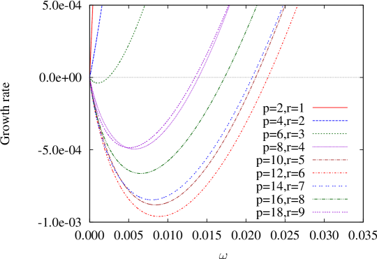
Refer to caption
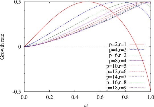
Figure 1: Growth rates to the average symbol weight distributions for the (2,8)28(2,8)-regular non-binary cluster LDPC code ensembles with the cluster size (p,r)=(2,1),(4,2),,(18,9)𝑝𝑟2142189(p,r)=(2,1),(4,2),\dots,(18,9).
Refer to caption
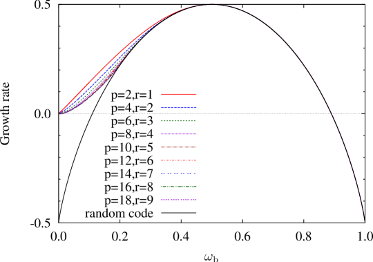
Figure 2: Growth rates to the average symbol weight distributions for the (2,8)28(2,8)-regular non-binary cluster LDPC code ensembles with the cluster size (p,r)=(2,1),(4,2),,(18,9)𝑝𝑟2142189(p,r)=(2,1),(4,2),\dots,(18,9).
Refer to caption
Figure 3: Growth rates to the average bit weight distributions for the (2,8)28(2,8)-regular non-binary cluster LDPC code ensembles with the cluster size (p,r)=(2,1),(4,2),,(18,9)𝑝𝑟2142189(p,r)=(2,1),(4,2),\dots,(18,9). The black solid curve (random code) gives the growth rate for the binary random code ensemble of rate 0.50.50.5.
Refer to caption
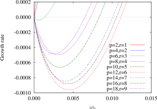
Figure 4: Growth rates to the average bit weight distributions for the (2,8)28(2,8)-regular non-binary cluster LDPC code ensembles with the cluster size (p,r)=(2,1),(4,2),,(18,9)𝑝𝑟2142189(p,r)=(2,1),(4,2),\dots,(18,9).
Refer to caption
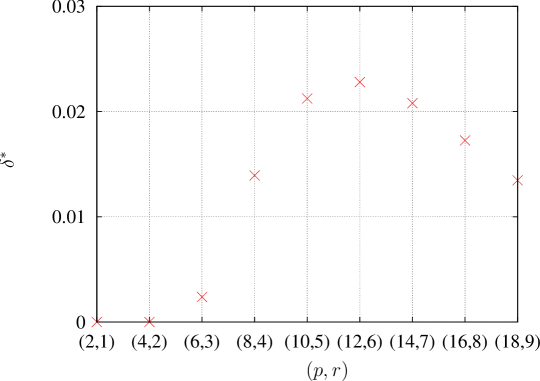
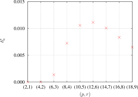
Figure 5: The normalized typical minimum distance δsuperscript𝛿\delta^{*} of the symbol weight distribution for the (2,8)-regular non-binary cluster LDPC code ensemble with the cluster size (p,r)=(2,1),(4,2),,(18,9)𝑝𝑟2142189(p,r)=(2,1),(4,2),\dots,(18,9).
Refer to caption
Figure 6: The normalized typical minimum distance δbsubscriptsuperscript𝛿b\delta^{*}_{\mathrm{b}} of the bit weight distribution for the (2,8)-regular non-binary cluster LDPC code ensemble with the cluster size (p,r)=(2,1),(4,2),,(18,9)𝑝𝑟2142189(p,r)=(2,1),(4,2),\dots,(18,9).

In this section, we show some numerical examples of the growth rates for the cluster non-binary LDPC code ensembles. As an example, we employ the (2,8)28(2,8)-regular non-binary cluster LDPC codes. To keep the design rate at half, we fix the ratio of the cluster size as p/r=2𝑝𝑟2p/r=2.

Figures 1 and 2 give the growth rates to the average symbol weight distributions for the cluster size (p,r)=(2,1),(4,2),,(18,9)𝑝𝑟2142189(p,r)=(2,1),(4,2),\dots,(18,9). As shown in Corollary 3, γ(1)𝛾1\gamma(1) tends to the design rate 0.50.50.5. From Figure 2, we see that the slop of the growth rate at ω=0𝜔0\omega=0 are negative and the normalized typical minimum distance δsuperscript𝛿\delta^{*} is strictly positive for (p,r)=(6,3),(8,4),,(18,9)𝑝𝑟6384189(p,r)=(6,3),(8,4),\dots,(18,9). This confirms Corollary 5.

Figures 3 and 4 give the growth rates to the average bit weight distributions for the cluster size (p,r)=(2,1),(4,2),,(18,9)𝑝𝑟2142189(p,r)=(2,1),(4,2),\dots,(18,9). The black solid curve in Figure 3 shows the growth rate of the binary random code ensemble of rate 0.50.50.5. As shown in Corollary 4, γb(1)subscript𝛾b1\gamma_{\mathrm{b}}(1) tends to 0.50.5-0.5. Moreover, we see that the curves in ωb>1/2subscript𝜔b12\omega_{\mathrm{b}}>1/2 converge to the growth rate of the binary random code ensemble. From Figure 4, we see that the slop of the growth rate at ωb=0subscript𝜔b0\omega_{\mathrm{b}}=0 are negative and the normalized typical minimum distance δbsubscriptsuperscript𝛿b\delta^{*}_{\mathrm{b}} is strictly positive for (p,r)=(6,3),(8,4),,(18,9)𝑝𝑟6384189(p,r)=(6,3),(8,4),\dots,(18,9). This confirms Corollary 5.

Figures 5 and 6 give the normalized typical minimum distance δsuperscript𝛿\delta^{*} and δbsubscriptsuperscript𝛿b\delta^{*}_{\mathrm{b}} of the symbol and bit weight distribution, respectively, for the cluster size (p,r)=(2,1),(4,2),,(18,9)𝑝𝑟2142189(p,r)=(2,1),(4,2),\dots,(18,9). From Figures 5 and 6, we see that the normalized typical minimum distances δsuperscript𝛿\delta^{*} and δbsubscriptsuperscript𝛿b\delta^{*}_{\mathrm{b}} does not monotonically increase with the size of cluster (p,r)𝑝𝑟(p,r). In this case, the normalized typical minimum distances δ,δbsuperscript𝛿subscriptsuperscript𝛿b\delta^{*},\delta^{*}_{\mathrm{b}} have the local maximum at (p,r)=(12,6)𝑝𝑟126(p,r)=(12,6).

V Conclusion

In this paper, we have derived the average weight distributions for the irregular non-binary cluster LDPC code ensembles. Moreover, we have given the exponential growth rate of the average weight distribution in the limit of large code length. We have shown that there exist (2,dc2subscript𝑑c2,d_{\mathrm{c}})-regular non-binary cluster LDPC code ensembles whose normalized typical minimum distances are strictly positive.

Acknowledgment

This work was supported by Grant-in-Aid for JSPS Fellows. The work of K. Kasai was supported by the grant from the Storage Research Consortium.

References

  • [1] R. G. Gallager, Low Density Parity Check Codes.   in Research Monograph series, MIT Press, Cambridge, 1963.
  • [2] T. Richardson, M. A. Shokrollahi, and R. Urbanke, “Design of capacity-approaching irregular low-density parity-check codes,” IEEE Trans. Inf. Theory, vol. 47, no. 2, pp. 619–637, Feb. 2001.
  • [3] M. Davey and D. MacKay, “Low-density parity check codes over GF(q𝑞q),” IEEE Commun. Lett., vol. 2, no. 6, pp. 165–167, Jun. 1998.
  • [4] X.-Y. Hu, E. Eleftheriou, and D. Arnold, “Regular and irregular progressive edge-growth Tanner graphs,” IEEE Trans. Inf. Theory, vol. 51, no. 1, pp. 386–398, Jan. 2005.
  • [5] V. Savin and D. Declercq, “Linear growing minimum distance of ultra-sparse non-binary cluster-LDPC codes,” in Proc. 2011 IEEE Int. Symp. Inf. Theory (ISIT), Aug. 2011, pp. 523–527.
  • [6] G. Miller and D. Burshtein, “Bounds on the maximum-likelihood decoding error probability of low-density parity-check codes,” IEEE Trans. Inf. Theory, vol. 47, no. 7, pp. 2696–2710, Nov. 2001.
  • [7] C. Di, T. Richardson, and R. Urbanke, “Weight distribution of low-density parity-check codes,” IEEE Trans. Inf. Theory, vol. 52, no. 11, pp. 4839–4855, Nov. 2006.
  • [8] T. Richardson and R. Urbanke, Modern Coding Theory.   Cambridge University Press, Mar. 2008.
  • [9] K. Kasai, C. Poulliat, D. Declercq, and K. Sakaniwa, “Weight distribution of non-binary LDPC codes,” IEICE Trans. Fundamentals, vol. E94-A, no. 4, pp. 1106–1115, Apr. 2011.
  • [10] I. Andriyanova, V. Rathi, and J.-P. Tillich, “Binary weight distribution of non-binary ldpc codes,” in Proc. 2009 IEEE Int. Symp. Inf. Theory (ISIT), June-July 2009, pp. 65–69.
  • [11] D. Burshtein and G. Miller, “Asymptotic enumeration methods for analyzing LDPC codes,” IEEE Transactions on Information Theory, vol. 50, no. 6, pp. 1115–1131, Jun. 2004.
  • [12] K. Kasai, T. Awano, D. Declercq, C. Poulliat, and K. Sakaniwa, “Weight distribution of multi-edge type LDPC codes,” IEICE Trans. Fundamentals, vol. E93-A, no. 11, pp. 1942–1948, Nov. 2010.