Evolution of blue supergiants and $\alpha$ Cygni variables; Puzzling CNO surface abundances

Abstract

A massive star can enter the blue supergiant region either evolving directly from the main-sequence, or evolving from a previous red supergiant stage. The fractions of the blue supergiants having different histories depend on the internal mixing and mass-loss during the red supergiant stage. We study the possibility to use diagnostics based on stellar pulsation to discriminate blue supergiants having different evolution histories. For this purpose we have studied the pulsation property of massive star models calculated with the Geneva stellar evolution code for initial masses ranging from 8 to 50 M_⊙ with a solar metallicity of $Z=0.014$. We have found that radial pulsations are excited in the blue-supergiant region only in the models that had been red-supergiants before. This would provide us with a useful mean to diagnose the history of evolution of each blue-supergiant. At a given effective temperature, much more nonradial pulsations are excited in the model after the red-supergiant stage than in the model evolving towards the red-supergiant. The properties of radial and nonradial pulsations in blue supergiants are discussed. Predicted periods are compared with period ranges observed in some $\alpha$-Cygni variables in the Galaxy and NGC 300. We have found that blue supergiant models after the red-supergiant stage roughly agree with observed period ranges in most cases. However, we are left with the puzzle that the predicted surface N/C and N/O ratios seem to be too high compared with those of Deneb and Rigel.

1 Introduction

The post-main-sequence evolution of massive stars depends sensitively on the helium core mass and its ratio to the envelope mass, which in turn depends on still poorly understood phenomena such as mixings in the radiative layers (core overshooting and rotational mixing) and wind mass loss. Recent evolution models with a solar metallicity of $Z=0.014$ by Ekström et al. (2012) indicate that a star with a sufficiently large initial mass undergoes a blue-red-blue (or blue-loop) evolution before central helium exhaustion; i.e., the star ignites He in the center in the blue supergiant (BSG) stage, evolves to the red-supergiant (RSG) region, and returns to the blue supergiant (BSG) region during core He-burning. The lowest initial-mass for the blue-red-blue evolution depends on the degree of mixing in radiative layers and the strength of wind mass loss. Ekström et al. (2012)’s results indicate the lower bound to be about 20 M_⊙. The mass limit is lowered if higher mass-loss rates in the RSG phase is assumed (Georgy, 2012; Salasnich et al., 1999; Vanbeveren et al., 1998).

Thus, luminous BSGs consist of two groups having different evolution histories: one group are evolving red-wards just after the termination of main-sequence, while another group have evolved back from the RSG stage. The BSGs belonging to the latter group have significantly reduced envelope mass and the surface is contaminated by the CNO-processed matter due to a dredge-up in the RSG stage and a significant mass loss. The fraction of each group depends on the internal mixing in the radiative layers and the strength of stellar wind and metallicity. In other words, if we can distinguish the two kinds of BSGs, it would be very useful for constraining the mixing in radiative layers and wind parameters. Furthermore, the fraction relates to the relative frequencies of different types of core-collapse supernovae such as IIP, IIL, IIb, Ib and Ic (e.g., Georgy et al., 2012; Yoon et al., 2012; Eldridge et al., 2013; Vanbeveren et al., 2012) and the ratio of blue to red supergiants (e.g., Meylan & Maeder, 1983; Langer & Maeder, 1995; Eggenberger et al., 2002).

One way to distinguish the two groups is to obtain their surface abundances of the CNO elements. This has been pursued intensively by many authors; e.g., the VLT-FLAME survey (Hunter et al., 2009), Przybilla et al. (2006) and Takeda & Takada-Hidai (2000). Although the majority of BSGs show enhanced N/C ratios, theoretical interpretations were somewhat hampered by the variety of rotation velocities which yield various degree of internal mixings in the main-sequence stage, and possible effect of close binaries and magnetic fields.

We propose, in this paper, another way to distinguish the two groups of BSGs by using stellar pulsation; i.e., we will argue that if they show (radial) pulsations, they must have been red supergiants before. It is known that many luminous ($\log L/{\rm L}_{\odot}\ga 4.6$) BA-supergiants in our Galaxy and Magellanic Clouds show micro variations in luminosity and in radial velocities; they are called $\alpha$-Cygni variables (e.g., van Leeuwen, et al., 1998). In addition, Bresolin et al. (2004) found that a fraction of blue supergiants in the galaxy NGC 300 are such variables and at least two of those show clear radial pulsation properties. The NGC 300 BSGs would be particularly useful for constraining evolutionary models, because of the homogeneity of the data and less ambiguities in luminosity.

The pulsation not only provides us with diagnostic means, it might also have effects on stellar winds from massive stars, as Aerts et al. (2010b) found a relation between episodic changes in mass loss and the 37 day pulsation of the luminous blue supergiant HD 50064. They suggested that the pulsation is a radial strange-mode pulsation, which we confirm in this paper.

The paper is organized as follows: evolution models of massive stars and the excitation of radial pulsations in these models are discussed in §2. The properties of radial and nonradial pulsations and their excitation mechanisms are discussed in §3. In §4 we compare observed semi-periods of $\alpha$-Cygni variables with theoretical ones and discuss surface compositions. Our conclusion is given in §5.

2 Massive star evolution and the stability to radial pulsations

Evolutionary models have been calculated by the Geneva evolution code with the same input physics as those described in Ekström et al. (2012). The initial abundances adopted are $(X,Z)=(0.720,0.014)$ with a solar mixture for the heavy elements (Asplund, Grevesse, & Sauval, 2005; Cunha, Hubeny, & Lanz, 2006, for the Ne abundance). A core overshooting of 0.1 pressure scale height is included. Stellar mass loss rate for a given position on the HR diagram and current mass is obtained from the prescriptions described in Ekström et al. (2012) (Except for $14\,M_{\odot}$ models, see below).

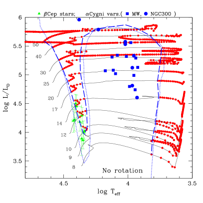
Figure 1: Evolutionary tracks for massive models without rotation for a chemical composition of $(X,Z)=(0.72,0.014)$ and the stability boundary (dashed line) for low-order radial pulsations. For models with $M_{\rm i}\geq 25$ M_⊙ the stability boundary is determined for models evolving red-ward for the first time. Dotted line indicates the stability boundary for $(X,Z)=(0.70,0.02)$ (GN93 abundance Grevesse & Noels, 1993). Red dots along evolutionary tracks indicate the positions of the models in which at least one radial modes is excited. Also plotted are some of the observed $\alpha$ Cygni variables (filled circles and squares) and $\beta$ Cephei variables (triangles with error bars). For the parameters of the Galactic $\alpha$ Cygni variables, we referred to various literature including that listed in Table 2, and Kudritzki et al. (1999). For $\alpha$ Cygni variables in NGC 300 we referred to Bresolin et al. (2004) and Kudritzki et al. (2008). Parameters adopted for $\beta$ Cephei variables are listed in Table 1. Small jumps during the Cepehid loops for $M_{\rm i}\leq 10M_{\odot}$ are produced by quick extensions of the convective core.

Table 1: Parameters of $\beta$ Cephei variables^∗ adopted in Fig. 1

Name	$\log T_{\rm eff}$	$\pm$	$\log L/L_{\odot}$	$\pm$	ref
15 CMa	4.408	0.021	4.50	0.16	a
$\beta$ CMa	4.40	0.04	4.45	0.20	b
BW Vul	4.358	0.028	4.29	0.14	c
KZ Mus	4.415	0.012	4.22	0.20	d
V433 Car	4.425	0.012	4.20	0.2	d
12 Lac	4.374	0.019	4.18	0.16	e
$\delta$ Cet	4.339	0.008	4.02	0.05	f
$\nu$ Eri	4.360	0.022	3.89	0.29	g
16 Lac	4.345	0.015	4.0	0.2	h
HD129929	4.350	0.015	3.86	0.15	i

a=Shobbrook et al. (2006), b=Mazumdar et al. (2006), c=Fokin et al. (2004), d=Handler et al. (2003), e=Handler et al. (2006), f=Aerts et al. (2006), g=De Ridder et al. (2004) , h=Thoul et al. (2003), i=Dupret et al. (2004)
^∗This is a very incomplete sample of Galactic $\beta$ Cep variables collected only for illustrative purpose in Fig. 1.

Fig. 1 shows evolutionary tracks up to the central helium exhaustion calculated without including rotational mixing for initial masses of 8, 9, 10, 12, 14, 17, 20, 25, 30, 40, and 50 M_⊙. For $M_{\rm i}\geq 12$ M_⊙, the helium burning starts when stars are evolving in the blue supergiant (BSG) region after the termination of main-sequence stage. As He burns in the center, they evolve into the red supergiant (RSG) stage. Stars with $M_{\rm i}\geq 30$ M_⊙ evolve back to the BSG region (blue-loop) before the helium is exhausted in the center. A star starts a blue-loop when it loses enough mass in the RSG stage (Fig. 2). This has an important consequence for the stability of radial pulsations.

We have performed a stability analysis of radial pulsations for selected evolutionary models. The method is described in Saio, Winget, & Robinson (1983), where the perturbation of the divergence of convective flux and the effect of rotation is neglected. The latter is justified because rotation is always slow in the envelope of supergiants (this is also true in our models with rotation; see Appendix), where pulsations have appreciable amplitudes. The effect of convection is neglected because the theory for the convection-pulsation coupling is still infant. Since the convective flux is less than 50% of the total flux in the convection zones in the envelope of blue supergiants, we do not think that neglecting the convection-pulsation coupling affects significantly our results.

The outer boundary is set at an optical depth of $\sim 10^{-4}$. We have adopted the outer mechanical condition that the Lagrangian perturbation of the gas pressure goes to zero.

The red dots along evolutionary tracks in Fig. 1 indicate the positions of the models that are found to have at least one excited radial mode. The dashed line in Fig. 1 indicates the stability boundary of radial low-order pulsations, which are appropriate for the Cepheids and $\beta$ Cephei variables. For models with $M_{\rm i}\geq 30$ M_⊙, which make blue-red-blue evolution, the part evolving toward the RSG region (first crossing) was used to obtain the stability boundary. For comparison, the stability boundary for models with the abundance $Z=0.02$ (Saio, 2011) with GN93 mixture (Grevesse & Noels, 1993) is also shown by a dotted line.

The nearly vertical ‘finger’ of the instability boundary around $\log T_{\rm eff}\sim 4.3-4.4$ corresponds to the $\beta$ Cephei instability region (excited by the $\kappa$-mechanism at the Fe-opacity bump around $T\sim 2\times 10^{5}$K), while the vertical boundary at $\log T_{\rm eff}\sim 3.8$ is the blue edge of the Cepheid instability strip, in which pulsations are excited at the second helium ionization zone. (No red-edge is obtained because our pulsation analysis does not include the coupling between pulsation and convection.)

The boundary for the $\beta$ Cephei instability region depends on the metal abundance. The positions of some Galactic $\beta$ Cephei stars are shown in Fig. 1 by filled triangles with error bars. Comparing the distribution of the $\beta$ Cephei variables with the stability boundaries for $Z=0.014$ (dashed line) and $Z=0.02$ (dotted line), we see that the most appropriate heavy-element abundance for the Galactic $\beta$ Cephei variables seems to be slightly larger than $Z=0.014$. The other part of the instability boundary hardly depends on the metallicity.

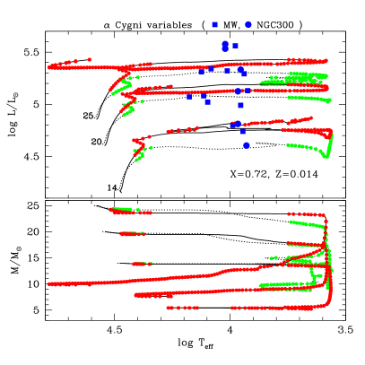
Figure 2: Top panel shows evolutionary tracks for $M_{\rm i}=25,20$, and 14 M_⊙, and the bottom panel shows the decrease of mass during the evolution for each initial mass. Solid and dotted lines are for models with and without rotation, respectively. Rotation rates are assumed to be 40% of the critical rate at the zero-age main-sequence stage. Red and green dots along each line indicate models in which at least one radial pulsation mode is excited. Some of the $\alpha$ Cygni variables in our Galaxy (filled squares) and in the galaxy NGC 300 (filled circles) are also plotted.

The instability boundary for radial pulsations by (weakly non-adiabatic) $\kappa$-mechanisms have steep gradients in the HR diagram as seen in the less luminous part ($\log L/{\rm L}_{\odot}\la 5$) of Fig. 1, where the instability boundaries for $Z=0.014$ and 0.02 are shown by broken lines. This comes from the requirement that the pulsation period should be comparable to the thermal timescale at the zone where the $\kappa$-mechanism works (e.g., Cox, 1974). At high luminosity, the instability boundary is nearly horizontal. This is associated with the strange modes that occur if $L/M\ga 10^{4}\,{\rm L}_{\odot}/{\rm M}_{\odot}$ (e.g., Gautschy & Glatzel, 1990; Glatzel, 1994; Saio et al., 1998, and discussion below).

In the BSG models evolving toward the RSG stage no radial modes are excited between the red-boundary of the $\beta$ Cephei instability region and the Cepheid blue-edge, because $L/M$ is not sufficiently large for the strange mode mechanism to work. Models with $M_{\rm i}\geq 30$ M_⊙ return to the BSG region (blue-loop) from the RSG region before core-helium exhaustion. Radial pulsations are excited in the models on the blue-loop; this is due to the fact that a significant mass is lost in the RSG stage and hence the $L/M$ ratio has increased considerably (Fig. 2). We can identify $\alpha$ Cygni variables (especially if radial pulsations are involved) to be core-helium burning stars on the blue-loop returned from the RSG stage. However, the luminosity of the track for $M_{\rm i}=30\,{\rm M}_{\odot}$ is still too high to be consistent with the distribution of $\alpha$ Cygni variables on the HR diagram. The discrepancy can be solved by taking into account rotational mixing (Ekström et al., 2012), or assuming a strong mass loss caused by Roch-Lobe overflow in the RSG stage. We consider the effect of rotational mixing in this paper.

We have calculated evolution models for $M_{\rm i}=25,20$, and 14 M_⊙ with rotational mixing, and examined the stability of radial pulsations for those models. The ways to treat rotation and the mixing are the same as Ekström et al. (2012); the rotation speed was assumed to be 40% of the critical one at the zero-age main-sequence stage. The results are shown in Fig. 2. The rotational mixing makes helium core and hence luminosity larger in the post main-sequence evolution for a given initial mass. A smaller ratio of the envelope to core mass makes the red-ward evolution faster; i.e., less He is consumed in the first BSG stage. (Note that dotted lines in the bottom panel of Fig. 2 tend to lose more mass as a function of $T_{\rm eff}$ in the first crossing, indicating the evolution to be slow there without rotational mixing). Also, the higher luminosity enhances stellar winds so that the star starts blue loop earlier, well before the central He exhaustion. We note that the important effect of rotation comes from the mixing that enlarges He core, but not from the centrifugal force. Therefore, a similar evolution is possible even without including rotation if a more extensive core overshooting is assumed. For $M_{\rm i}=20\,M_{\odot}$, for example, an extensive blue-loop occurs before He exhaustion if a core overshooting larger than $\sim 0.4\,H_{p}$ is included without rotational mixings; if a mass-loss rate is enhanced by a factor of 5, for example, it occurs for a overshooting larger than $\sim 0.35\,H_{p}$.

The non-rotating evolutionary track of $M_{\rm i}=14\,$M_⊙ passes, in the first crossing, around the lower bound of the distribution of the $\alpha$ Cygni variables ($\log L/{\rm L}_{\odot}\ga 4.6$). However, it does not come back to blue region even if rotation is included with our standard parameters. It does make a blue loop as shown in Fig. 2, if the rate of cool winds is increased by a factor of five as in Georgy (2012). Such an increase is reasonable since there are many theoretical and observational arguments of sustaining higher mass loss rates during the red supergiant phase. From a theoretical point of view, Yoon & Cantiello (2010) have studied the consequence of a pulsation driven mass loss during the red supergiant phase. They showed that using empirical relations between the pulsation period and the mass loss rates, the mass loss rates could be increased by quite large factors largely exceeding a factor 5 at least during short periods.

From an observational point of view, the circumstellar environment of red supergiants clearly indicates that some stars undergo strong mass loss outbursts. For instance, VY CMA (M2.5-5Iae) which has a current mass loss rate of 2-4 10^-4M_⊙ per year (Danchi et al., 1994) is surrounded by a very inhomogeneous nebula likely resulted from a series of episodic mass ejections over the last 1000 yr (Smith, Hinkle, & Ryde, 2009). It is estimated that the mass loss rates between a few hundred and 1000 yr ago was 1-2 10^-3M_⊙ per year, thus between 2.5 and 10 times greater than the present rate.

We also note that mass loss rates obtained by van Loon et al. (2005) for dust enshrouded red supergiants are larger by a factor up to 10 compared with the rates estimated from the empirical relations given in (1988)

In the present standard computation we used the prescription by (1988). The arguments above indicate that using mass loss rates increased by a factor 5 is not beyond the uncertainty in our present state of knowledge on the mass loss rates of red supergiants.

It is interesting to note that for the case of 14 M_⊙ not all models on the blue-loop excite pulsations. More precisely, no radial modes are excited in the blueward evolution at $\log T_{\rm eff}\approx 4$ ($\log L/M=4.03$). Only in the second redward evolution (third crossing), a radial mode is excited around similar effective temperature; this time, models have slightly higher $L/M$ ($\log L/M=4.08$).

The fact that no $\alpha$ Cygni variables are observed below a luminosity limit of about $\log L/{\rm L}_{\odot}\approx 4.6$ does not necessarily means that stars below that limit have no blue-loop. Even if they make a blue-loop evolution, their $L/M$ ratio would be too small for pulsations to be excited.

The observed properties of $\alpha$ Cygni variables can be well explained if these stars are core He-burning stars on the blue-loop. This supports the presence of considerable mixing and possibly cool winds stronger than adopted in Ekström et al. (2012). Note that an increased mass loss during the RSG phase seems to be also required in order to reproduce the observed positions of $\alpha$ Cyg variables at high luminosity. (Indeed, the models in Ekström et al. (2012) have a mass-loss rate increased by a factor of 3 for models more massive than 20 M_⊙ during the RSG phase).

From the ratio of the evolution speeds between the first (red-ward) and second (blue-ward) crossings we can estimate the probability for a BSG to be on the first crossing. At positions of typical BSGs, Rigel and Deneb (see Table 2 below), for example, the probabilities are 45% and 98% , respectively, for $M_{i}=20\,M_{\odot}$, while they are 15% and 50% or $M_{i}=25\,M_{\odot}$; in both cases rotational mixings are included. If we use models without rotation, the probabilities are nearly unity for both stars and for both initial masses, because in this case the second crossings occur very swiftly after the core He exhaustion.

3 Properties of pulsations in BSG models

In this section we discuss the properties and excitations of radial and nonradial pulsations in BSG models with rotational mixing. Although these models start with 40% of the critical rotation at the zero-age main-sequence stage, the rotation speeds in the envelopes in all the supergiant models are very low as discussed in Appendix, so that we did not include the rotation effects in our pulsation analyses.

3.1 Radial pulsation

Figure 3: Normalized pulsation (angular) frequency, $\omega_{\rm r}$ (the real part of complex eigenfrequency $\omega$), for BSG models of $M_{i}=25M_{\odot}$ with rotation are plotted as functions of $\log T_{\rm eff}$. The top and the bottom panels are for models evolving toward and from the RSG stage, respectively. The masses in the latter models are significantly reduced from the former models, while the luminosities are comparable. Filled circles indicate excited modes, while ‘$\times$’ and ‘+’ are damped modes. The symbol ‘+’ is used for the thermal damping modes with $2.0\geq\omega_{i}/\omega_{r}\geq 0.5$, for which damping time is comparable to the pulsation period (modes with $\omega_{i}>2\omega_{r}$ are not plotted).

In our linear pulsation analysis, the temporal dependence of variables is set to be $\exp(i\sigma t)$, where $\sigma(=\sigma_{\rm r}+i\sigma_{\rm i})$ is a complex frequency obtained as the eigenvalue for the set of homogeneous differential equations for linear pulsations. The real part $\sigma_{\rm r}$ gives the pulsation period ($2\pi/\sigma_{\rm r}$) and the imaginary part $\sigma_{i}$ gives the stability of the pulsation mode (excited if $\sigma_{\rm i}<0$). We use the symbol $\omega~{}(=\omega_{\rm r}+i\omega_{\rm i})$ for normalized (complex) frequency; i.e.,

$$\omega=\omega_{\rm r}+i\omega_{\rm i}=(\sigma_{\rm r}+i\sigma_{\rm i})/\sqrt{GM/R^{3}}$$

with $G$ being the gravitational constant and $R$ the stellar radius.

Fig. 3 shows $\omega_{\rm r}$, normalized pulsation frequency, for low-order radial pulsation modes in the BSG models of $M_{\rm i}=25\,{\rm M}_{\odot}$ evolving toward the RSG stage (top panel) and evolving from the RSG on a blue-loop (bottom panel). Filled circles indicate excited modes, while ‘$\times$’ and ‘+’ are damped modes. In the top panel, the normalized frequency of each mode varies regularly as a function of $\log T_{\rm eff}$, keeping the order such that the lowest frequency is the fundamental mode (F) with no node in the amplitude distribution, next one is the first overtone (1Ov) with one node, and so on. (The ordering is strictly hold only in adiabatic pulsations). The fundamental mode in the range $\log T_{\rm eff}\geq 4.34$ is excited by the Fe-opacity bump as the models are in the $\beta$ Cephei instability region. The other modes in the top panel are all damped. A very low frequency mode which appears in the range $\log T_{\rm eff}\la 4.0$ of the top panel is a mode associated with thermal (damping) wave, so that it is strongly damped. The symbol ’+’ is used in Fig. 3 for strongly damped modes with $2.0\geq\omega_{i}/\omega_{r}\geq 0.5$ (modes with $\omega_{i}>2\omega_{r}$ are not plotted).

In models with high $L/M$ ratios as shown in the bottom panel of Fig. 3, the frequencies of thermal modes enter into the frequency range of dynamical pulsations, and $\omega_{i}$ decreases (the damping time becomes longer) so that the two types of pulsations become indistinguishable.

In the bottom panel of Fig. 3 for models on the blue-loop, at least one mode is excited throughout the $T_{\rm eff}$ range (three modes are excited in most part). The frequency of each mode varies in a more complex way; the mode ordering rule is lost, additional mode sequences appear, and frequent mode crossings occur, etc. The appearance of such complex behaviors is related with strange modes. The strange modes may be defined as modes which are not seen in adiabatic analyses. With this definition the thermal damping modes also belong to strange modes, but we are more interested in another type of strange modes which are excited by a special instability even when the thermal time goes to zero which was first recognized by Gautschy & Glatzel (1990). (We will discuss the mechanism briefly below). Sequence S2 in Fig. 3 corresponds to such a strange mode. Sequence S1, another strange mode, is somehow related with the lowest frequency mode ($\omega_{r}<0.05$) seen in the range $\log T_{\rm eff}\la 4.0$ of the top panel. The two sequences is connected in the RSG stage, which is not shown in Fig. 3. The S1 mode, as discussed below, seems to be excited mainly by enhanced $\kappa$-mechanism at the Fe-opacity bump.

The main difference between the models in the top and in the bottom panels of Fig. 3 is the luminosity to mass ratio; models in the bottom panel (on the blue-loop) have $L/M\sim 2.0\times 10^{4}\,{\rm L}_{\odot}/{\rm M}_{\odot}$, while in the top panel $L/M\sim 1.1\times 10^{4}\,{\rm L}_{\odot}/{\rm M}_{\odot}$. A higher $L/M$ ratio makes pulsations more nonadiabatic. This can be understood from a linearized form of energy conservation for stellar envelope;

$$T{\partial\delta S\over\partial t}=-{L\over M}{\partial\over\partial q}\left({\delta L\over L}\right),$$ (1)

where $\delta$ means the Lagrangian perturbation of the next quantity, $S$ is the entropy per unit mass, and $q\equiv M_{r}/M$. The above equation indicates that generally a high value of $L/M$ generates a large entropy change and hence large nonadiabatic effects.

A large $L/M$ ratio has also a significant effect on the envelope structure by enhancing the importance of radiation pressure. Combining a hydrostatic equation with a radiative diffusion equation for the envelope of a static model, we obtain a relation

$${dP_{\rm gas}\over dP}=1-{\kappa\over 1.3\times 10^{4}{\rm(cm^{2}/g)}}{L_{\rm rad}/L_{\odot}\over M/M_{\odot}},$$ (2)

where $P_{\rm gas}$ is the gas pressure, $P$ is the total pressure, $\kappa$ is the opacity in units of ${\rm cm^{2}g^{-1}}$, and $L_{\rm rad}$ is the local radiative luminosity. This equation indicates that the inward increase of the gas pressure is hampered or inverted if $L_{\rm rad}/M\ga 10^{4}\,{\rm L}_{\odot}/{\rm M}_{\odot}$, and the effect is strong where the opacity is large. A radiation pressure dominated zone is formed around an opacity peak in the stellar envelope with a $L/M$ ratio larger than $\sim 10^{4}\,{\rm L}_{\odot}/{\rm M}_{\odot}$. We note that if the second term on the right hand side of equation (2) is sufficiently large, a density inversion is formed.

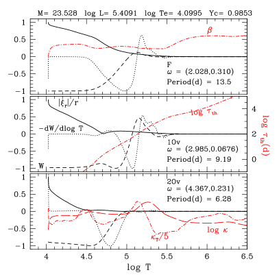
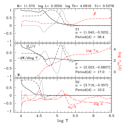
Figure 4: Pulsational displacement $\xi_{r}$, work $W$, and differential work $-dW/d\log T$ for the three lowest frequency modes are shown as functions of temperature in BSG models before (left panel) and after (right panel) the RSG stage. These quantities are normalized such that the maximum absolute value is unity. The two models have similar effective temperatures of $\log T_{\rm eff}\approx 4.1$. The mode name given in each panel corresponds to the name given in Fig. 3. The runs of $\beta=P_{\rm gas}/P$, $\log\kappa$, and $\kappa_{T}=(\partial\ln\kappa/\partial\ln T)_{\rho}$, and thermal time $\tau_{\rm th}$ (in days) defined by eq. (5) are also shown. For $\tau_{\rm th}$ the right-side vertical scale of each panel should be referred.

Fig. 4 shows the properties of three pulsation modes F, 1Ov, and 2Ov in a BSG model (with 23.5 M_⊙) before the RSG stage (left panels) and S1, F, and S2 modes in a BSG model (with 11.6 M_⊙) on the blue-loop after the RSG stage (right panels). Both models have a similar effective temperature of $\log T_{\rm eff}\approx 4.1$. Each panel shows the runs of fractional displacement, $|\xi_{r}/r|$ (solid line), work $W(r)$ (dashed line), and differential work $-dW/d\log T$ (dotted line). The work is defined as

$$W(r)=4\pi\int_{0}^{r}Pr^{2}{\rm Im}\left({\delta P^{*}\over P}{\delta\rho\over\rho}\right)dr,$$ (3)

where $\delta P$ and $\delta\rho$ are the Lagrangian perturbations of the pressure and the density, respectively, and the superscript ^∗ indicates the complex conjugate of the quantity. (In the nonadiabatic linear pulsation analysis, we employ complex representations). The layers with $dW/dr\propto-dW/d\log T>0$ (dotted lines) contribute to drive the pulsation. The net effect of driving and damping through the stellar interior appears in the surface value of the work, $W(R)$; if $W(R)>0$ the pulsation mode is excited. The amplitude growth rate ($-\sigma_{i}/\sigma_{r}$) is related with $W(R)$ as

$$-{\sigma_{i}\over\sigma_{r}}={W(R)\over 2\sigma_{r}^{2}}\left[\int_{M}\mbox{\boldmath$\xi$}^{*}\cdot\mbox{\boldmath$\xi$}dM_{r}\right]^{-1},$$ (4)

where $\xi$ is pulsational displacement vector (for radial pulsations $\mbox{\boldmath$\xi$}=\xi_{r}\mbox{\boldmath$e$}_{r}$ with $\mbox{\boldmath$e$}_{r}$ being the unit vector in the radial direction). We assume the amplitude of an excited radial-pulsation mode to grow to be visible. All modes in the left panels of Fig. 4 are damped, while all modes in the right panels are excited.

Some structure variables are also shown in Fig. 4. Note that in the model on the blue-loop (right panel), $\beta(=P_{\rm gas}/P)$ is extremely small in the range $4.6\la\log T\la 5.4$, indicating $P\approx P_{\rm rad}$ there. The thermal time $\tau_{\rm th}$ is defined as

$$\tau_{\rm th}(r)=\int_{r}^{R}4\pi r^{2}{\rho C_{p}T\over L_{r}}dr,$$ (5)

where $C_{p}$ is the specific heat per unit mass at constant pressure. In the outermost layers with $\log T\la 4.7$, $\tau_{\rm th}$ is shorter than pulsation periods. The pulsations are locally very non-adiabatic there.

For the longest period modes shown in the top panels in Fig. 4, driving occurs around the Fe-opacity bump ($\log T\sim 5.0-5.4$). Since the thermal time there is longer than the pulsation periods, the driving can be considered as the ordinary $\kappa$-mechanism. Roughly speaking, the $\kappa$-mechanism works (under a weak nonadiabatic environment) if the opacity derivative with respect to temperature increases outward; i.e., $d\kappa_{T}/dr>0$ (Unno et al., 1989). We see that this rule is hold in the model before the RSG stage (left panel), in which the driving is overcome by radiative damping in the upper layers (where $d\kappa_{T}/dr<0$) so that the mode is damped. For the longest period mode (S1) in the model on the blue-loop (right panel), the driving zone extends out into zones where $\kappa_{T}$ decreases outward. Because of the extension of the driving zone, which is probably caused by small $\beta$, the mode is excited; i.e., the driving effect exceeds radiative damping in the upper layers. This mode is considered to be a strange mode because there is no adiabatic counterpart. However, the excitation is caused by the enhanced $\kappa$-mechanism, in accordance with the finding of Dziembowski & Sławińska (2005).

The modes in the middle panels in Fig. 4 are ordinary modes; the first overtone, 1Ov, for the model before the RSG stage (left panel) and fundamental mode, F, for the model on the blue-loop (right panel). For these modes the driving around $\log T\sim 4.5-4.8$ has some contribution in addition to the driving around the Fe-opacity bump. The mode in the left panel is damped because radiative damping between the two driving zones exceeds the driving effects, while the F mode in the right panel is excited. The driving in the low temperature zone should not be the pure $\kappa$-mechanism because the thermal time there is shorter than the pulsation periods. It should be somewhat affected by the strange mode instability, which is discussed below.

The mode in the left-bottom panel in Fig. 4, the second overtone (2Ov) of the model before the RSG stage is damped because of the lack of appreciable drivings. On the other hand, the S2 mode in the right-bottom panel is excited strongly in the zone ranging $4.3\la\log T\la 4.6$ (HeII ionization zone), where the thermal time $\tau_{\rm th}<1$ d is much shorter than the pulsation period (10.2 d). Because no heat blocking (which is essential for the $\kappa$-mechanism) occurs there, the driving mechanism must be the genuine strange-mode instability, which should work even in the limit of $\tau_{\rm th}\rightarrow 0$; NAR (Nonadiabatic reversible) approximation introduced by Gautschy & Glatzel (1990). In this limit, $\delta L=0$ (cf. eq. (1)). From this relation with the plane parallel approximation it is possible to derive an approximate relation of

$$\delta P\propto\pm i\kappa_{\rho}\kappa F_{\rm rad}{\delta\rho\over\rho}$$ (6)

(Saio, 2009), where $F_{\rm rad}$ is the radiative flux and $\kappa_{\rho}\equiv(\partial\ln\kappa/\partial\ln\rho)_{T}$. This relation indicates that a large phase difference arises between $\delta P$ and $\delta\rho$, which can lead to strong driving (and damping) according to the work integral given in eq. (3); in the limit of NAR approximation, if $\sigma$ is an eigenvalue, the complex-conjugate $\sigma^{*}$ is also an eigenvalue. This explains the strange mode instability (see Glatzel, 1994, for a different approach).

3.2 Nonradial pulsations

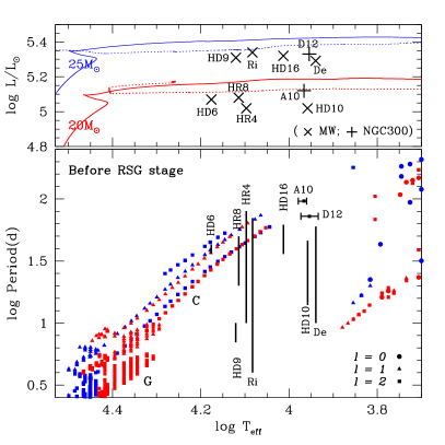
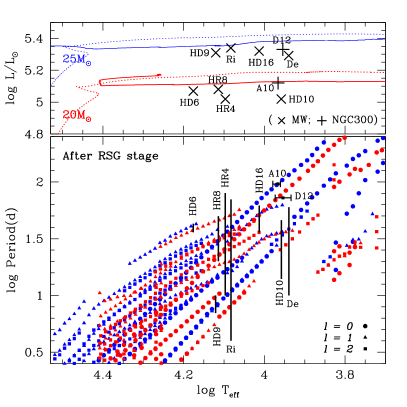
Figure 5: Evolutionary tracks of $M_{\rm i}=20$ and 25 M_⊙ models with rotation (top panels) and periods of pulsations excited (and visible satisfying eq.(7)) in the models (bottom panels) are compared with some of the $\alpha$ Cygni variables in our Galaxy and NGC 300. The left panels are for the models evolving toward the RSG stage, while the right panels are for the models on the blue loop from the RSG stage. The periods (or period ranges) are shown for some $\alpha$ Cygni variables in the Milky Way and in NGC 300 having luminosities within the considered range. Adopted parameters and periods are listed in Table 2. Names of stars; De=Deneb ($\alpha$ Cyg), HD10=HD100262, HD16=HD168607, Ri=Rigel ($\beta$ Ori), HR4=HD96919 (HR4338), HR8=HD199478 (HR8020), HD9=HD91619, and HD6=HD 62150; and A10 and D12 are star names in NGC 300 used by Bresolin et al. (2004).

The three dimensional property of a nonradial pulsation of a spherical star is characterized by the degree $l$ and the azimuthal order $m$ of a spherical harmonic $Y_{l}^{m}$ ($l=1$ for dipole and $l=2$ for quadrupole modes). There are two types of nonradial pulsations; p-modes (common to radial modes) and g-mode pulsations. The g-mode pulsations are possible only in the frequency range below the Brunt-Väisälä (or buoyancy) frequency (e.g., Unno et al., 1989; Aerts et al., 2010a). We have performed nonradial pulsation analyses based on the method described in Saio & Cox (1980), disregarding the effect of rotation. This is justified because we discuss the modes trapped in the envelope, where the rotation speed is very low as discussed in Appendix.

The properties and the stability of nonradial pulsations of supergiants are very complex because they have a dense core with very high Brunt-Väisälä frequency. All oscillations in the envelope with frequencies less than the maximum Brunt-Väisälä frequency in the core can couple with g-mode oscillations in the core through the evanescent zone(s) laying between the envelope and the core cavities. The coupling strength varies sensitively with the pulsation frequency and the interior structure of the star. Depending on the coupling strength, the relative amplitudes in the core and in the envelope vary significantly, and hence the stability changes.

Excitation by the $\kappa$-mechanism and the strange-mode instability works also for nonradial pulsations (Glatzel & Mehren, 1996). In addition, oscillatory convection mechanism (Shibahashi & Osaki, 1981; Saio, 2011) works in the convection zone associated with the Fe-opacity bump in the BSGs. Furthermore, the $\epsilon$-mechanism of excitation at the H-burning shell can excite nonradial modes which are strongly confined to a narrow zone there as shown by Moravveji et al. (2012b).

Among those nonradial modes which are excited, we restrict ourselves, in this paper, to possibly observable modes having the following properties:

$$l\leq 2\quad{\rm and}\quad f_{\rm amp}\equiv{|\xi_{r}|_{\rm surf}/R\over(|\xi_{r}|/r)_{\rm max}}>0.1,$$ (7)

where $\xi_{r}$ is the radial component of Lagrangian displacement, and the subscripts _surf and _max indicate the values at the stellar surface and at the maximum amplitude in the interior, respectively. The first requirement selects modes less affected by cancellation on the stellar surface. The second requirement excludes modes highly trapped in the interior; i.e., such oscillations hardly emerge to the surface. The second requirement excludes most of the g-modes excited in the core, because they are strongly trapped in the core having small ratios of $f_{\rm amp}<10^{-3}$.

Fig. 5 shows periods of excited nonradial dipole and quadrupole modes ($l=1,2$) (as well as radial modes) in models evolving toward RSG region (left panel) and in models on the blue-loop after the RSG stage (right panel) for $M_{\rm i}=20$ and 25 M_⊙ cases with rotation. Obviously, much more modes are excited in the BSG models after the RSG stage (on the blue-loop) in the period ranges of $\alpha$ Cygni variables.

In the BSG models before the RSG stage, excited observable modes are nonradial g-modes and oscillatory convection modes. Swarms of modes labeled as ’G’ in the left panel of Fig. 5 are g-modes excited by the Fe-opacity bump. For those oscillations, the amplitude is confined to the envelope by the presence of a shell convection zone above the H-burning shell (Saio et al., 2006; Godart et al., 2009; Gautschy, 2009), which prevents the oscillation from penetrating into and being damped in the dense core. The red edge for the group, $\log T_{\rm eff}\approx 4.3$, is bluer by 0.1 dex than that obtained by Gautschy (2009) for 25 M_⊙ models with $Z=0.02$. The difference can be attributed to the metallicity difference. These g-modes are probably responsible for the multi-periodic variations of the early BSG HD 163899 (B2Ib/II) (Saio et al., 2006) observed by the MOST satellite and some of the relatively less luminous early BSGs studied by Lefever et al. (2007).

The sequences labeled as ‘C’ in the left panel of Fig. 5 are oscillatory convection (g^-) modes associated with the convection zone caused by the Fe-opacity peak around $\log T\sim 5.2$ (the presence of such modes is discussed in Saio, 2011). The sequences terminate when the requirement of $f_{\rm amp}>0.1$ is not met anymore; i.e., beyond the termination the modes are trapped strongly in the convection zone.

The right panel for models after the RSG stage show many modes excited in the $T_{\rm eff}$–period range appropriate for the $\alpha$ Cygni variables. They are excited by different ways depending on the periods. Fig. 6 presents examples, in which amplitude and work curves are shown for the three dipole ($l=1$) modes excited (and $f_{\rm amp}>0.1$; eq.(7)) in a model of $M_{\rm i}=25\,{\rm M}_{\odot}$ at $\log T_{\rm eff}=4.031$ and $\log L/{\rm L}_{\odot}=5.374$. (Note that the mass of the model is reduced to 12.3 M_⊙ and hence the $L/M$ ratio is as high as $\sim 2\times 10^{4}\,{\rm L}_{\odot}/{\rm M}_{\odot}$.)

The top panel of Fig. 6 shows the lowest frequency dipole mode excited. This is one of the very rare cases in which the driving effect in the core is comparable with that in the envelope. In the envelope the amplitude is strongly confined to the Fe convection zone, which is characteristic of oscillatory convection modes. The envelope mode weakly couples with a core g-mode. Although the amplitude in the core is extremely small, the driving effect is comparable or larger than that in the envelope. In the hotter models contribution from the core is negligibly small, while as $T_{\rm eff}$ decreases the core contribution increases rapidly but the ratio $f_{\rm amp}$ soon becomes much smaller than 0.1.

The modes shown in the middle and the bottom panels of Fig. 6 are confined strongly to the envelope without any contribution from the core. The mode in the middle panel with a period of 26 days is excited around Fe-opacity bump at $T\sim 2\times 10^{5}$K and have large amplitude in the convection zone. The mode in the bottom panel with a period of 16.6 days corresponds to the S2 strange mode of radial pulsations shown in Fig. 4 (right-bottom panel), excited by the strange-mode instability around the He II ionization.

Three quadrupole ($l=2$) modes having periods and properties similar to those of dipole modes shown in Fig. 6 are also excited in the same model. However, the amplitudes of the two longer-period quadrupole modes are more strongly confined in the Fe-convection zone with amplitude ratios of $f_{\rm amp}\sim 0.05$ so that they do not meet the requirement given in eq. (7) and hence are not considered to be observable. Only the shortest period (16.1 days) mode with $f_{\rm amp}=1$ satisfies the requirement; this mode corresponds to the S2 mode.

In this model two radial strange modes belonging to S1 and S2 are also excited (Fig. 3) with periods of 54.1 and 16.3 days, respectively. Counting these excited observable pulsation modes, we expect a total of six pulsation periods; 54.1 and 16.3 days for the two radial pulsations, 46.3, 26.0, and 16.6 days for the three dipole modes, and 16.1 days for the quadrupole mode. The three very close periods of $\sim 16$ days would yield very long beat periods up to a few years. If these modes are simultaneously excited, the light curve would be extremely complex, which is just consistent with light curves of many $\alpha$ Cygni variables (e.g., van Leeuwen, et al., 1998).

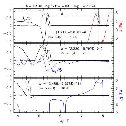
Figure 6: Three nonradial dipole ($l=1$) modes excited in a BSG model ($M_{\rm i}=25M_{\odot}$) after the RSG stage. Black solid lines show the real part of radial displacement, $\xi_{r}/r$. Dashed lines are for the work, $W(r)$ defined by eq. (3). Dotted lines are for the differential work $-dW/d\log T$. These quantities are plotted as functions of temperature in the model; they are normalized such that the maximum absolute value in the envelope is unity. The blue lines in the bottom and the middle panel show the run of square of Blunt-Väisälä frequency, $N^{2}$ (normalized by $GMR^{-3}$) and the opacity derivative $\kappa_{T}$, respectively. The red line in the top panel shows the run of nuclear energy generation rates $\epsilon$(erg g^-1s^-1).

4 Discussions

4.1 Comparison with periods of $\alpha$ Cygni variables

Despite the long history of observations for $\alpha$ Cygni variables, periods of variations are only poorly determined for most of the cases, hampered by complex and long-timescale light and velocity variations. Here we compare observed periods of relatively less luminous $\alpha$ Cygni variables shown in Fig. 5 with theoretical models of $M_{\rm i}=20,25\,M_{\odot}$ with rotational mixings.

Table 2: Adopted parameters and periods of $\alpha$ Cygni variables in the Galaxy and NGC 300

HD	$\log T_{\rm eff}$	$\log L$	ref	Peri.(d)	ref
MW Galaxy
34085 (Rigel)	4.083	5.34	a	4–70	b
62150	4.176	5.07	c	36–43	d
91619	4.121	5.31	e,f	7–10	g
96919 (HR4338)	4.097	5.02	f	10–80	g
100262	3.958	5.02	h	14–46	g,i
168607	4.013	5.32	c	36–62	d,j
197345 (Deneb)	3.931	5.29	k	10–60	l
199478 (HR8020)	4.114	5.08	m	20–50	n
NGC 300
A10	3.966${}^{+0.013}_{-0.006}$	5.12	o	96.1	p
D12	3.954${}^{+0.019}_{-0.020}$	5.33	o	72.5	p

a =Firnstein & Pryzbilla (2012);  b=Moravveji et al. (2012a); c=Leitherer & Wolf (1984); d=van Leeuwen, et al. (1998); e=Fraser et al. (2010); f=Kaltcheva & Scorcio (2010); g=Kaufer et al. (1997); h=Kaufer et al. (1996); i=Sterken (1977); j=Sterken et al. (1999); k=Schiller & Przybilla (2008); l=Richardson et al. (2011); m=Markova & Puls (2008); n=Percy et al. (2008); o=Kudritzki et al. (2008); p=Bresolin et al. (2004)

4.1.1 Deneb ($\alpha$ Cyg)

Deneb is the prototype of the $\alpha$ Cygni variables and has a long history of studies (see Richardson et al., 2011, for a review and references given). Although its light-curves are very complex, Richardson et al. (2011) obtained radial pulsation features at two short epochs. Strangely, however, the two epochs give two different periods; 17.8 days and 13.4 days. From the time-series analyses by Richardson et al. (2011) and Kaufer et al. (1996), we have adopted a period range of $10-60$ days. On the HR diagram Deneb is close to the blue-loop of $M_{\rm i}=25\,{\rm M}_{\odot}$ (Fig. 5); the current mass is about 12.7 M_⊙. Our model at $\log T_{\rm eff}\approx 3.93$ predicts the following periods for the excited modes; 127 & 49 days (radial), 42 days ($l=2$). The longest period is longer than the observed period range. The other two periods are in the longer part of the observed range. The periods of excited radial modes are much longer than the periods of radial pulsations, 17.8 and 13.4 days, obtained by Richardson et al. (2011). The reason for the discrepancy is not clear. Our model cannot explain the shorter part of the observed period range.

Gautschy (1992) tried to explain Deneb’s pulsations by nonradial strange modes and found that if the mass is less than 6.5 M_⊙, nonradial modes with various $l$ are excited. The required mass seems too small for the position of Deneb on the HR diagram. Recently, Gautschy (2009) found that nonradial modes of $l=1,2$ having periods consistent with the observed period range are excited by the H-ionization zone ($T\sim 10^{4}$ K) in models of 25 M_⊙ (evolving towards the RSG stage) with effective temperatures similar to the observed one. In our models, however, the H-ionization zone excites relatively short periods modes in cooler models with $\log T_{\rm eff}\sim 3.8-3.85$ (Fig. 5), which is inconsistent with Deneb. The reason for the difference is not clear; further investigations are needed.

4.1.2 Rigel ($\beta$ Ori)

The period range given in Table 2, $4-70$ days, is based on the recent analysis by Moravveji et al. (2012a). Kaufer et al. (1997)’ s analysis indicates a narrower range of $5-30$ days. The position on the HR diagram (Fig. 5) is consistent with a $M_{\rm i}=25\,{\rm M}_{\odot}$ model on the blue-loop after the RSG stage. Our model at $\log T_{\rm eff}\approx 4.08$ predicts excitation of the following visible modes: 40.1, 18.4, and 11.2 days (radial); 31.9, 16.4, and 11.4 days ($l=1$); 11.0 days ($l=2$). Our model predicts many pulsation modes in the longer part of the observed period range. Although no modes with periods shorter than 10 days are excited, those shorter periodicities might be explained by combination frequencies among excited modes. Moravveji et al. (2012b) proposed g-modes (with periods of longer than 20 days) excited by the $\epsilon$-mechanism at the H-burning shell. However, we think that those modes are invisible because the amplitude is very strongly confined to a narrow zone close to the H-burning shell.

4.1.3 HD 62150

The period range of HD 62150, $36-43$ days, is adopted from the analysis by van Leeuwen, et al. (1998) of the Hipparcos observations. In fact they obtained a 36.4 day period and a very small amplitude period of 43.0 days. These periods are consistent with nonradial (oscillatory convection mode) pulsations either in the first crossing toward the RSG stage, or on the blue loop of a model with $M_{\rm i}\approx 20M_{\odot}$ (Fig. 5). HD 62150 is, among the variables considered here, the only star which can be considered as in the first crossing stage.

4.1.4 Other stars in the MW

HD100262 has a similar $T_{\rm eff}$ to Deneb and has the same problem; i.e., the model cannot predict the shorter part of the observed period range. The period ranges of other stars, HD 168607, HR4338, HR 8020, and HD 91619 are roughly consistent with predicted periods of the models evolving on blue-loops from the RSG region.

4.1.5 A10 and D12 in NGC 300

Bresolin et al. (2004) found many $\alpha$-Cygni type variables among blue supergiants in the galaxy NGC 300. Among them, two stars, A10 and D12 show regular light curves with periods of 96.1 d and 72.5 d, respectively. The light curves look consistent with radial pulsations. Hence, according to our stability results, these stars must be on blue-loops after the RSG stage. Kudritzki et al. (2008) obtained heavy element abundances of $\log Z/Z_{\odot}=-0.04\pm 0.20$ for A10 and $-0.16\pm 0.15$ for D12, which indicate our models with $Z=0.014$ to be appropriate for these stars. The periods of A10 and D12 roughly agree with theoretical periods of radial pulsations obtained for $M_{\rm i}=20$ and 25 M_⊙ models (Fig. 5, right panel). These are strange modes excited at the Fe-opacity bump (Fig. 4) in BSG models after RSG stages. Because of the wind mass loss occurred in the previous stages, these models currently have masses of 8.8 and 12.7 M_⊙, respectively. Our models agree with Dziembowski & Sławińska (2005) who concluded that the pulsations of A10 and D12 should be strange modes in models with masses reduced significantly by mass loss.

However, Fig. 5 (right panel) indicates a discrepancy; in the HR diagram A10 and D12 are close to the evolutionary tracks of $M_{\rm i}=20$ ($\log L/{\rm L}_{\odot}\approx 5.1$) and $25\,{\rm M}_{\odot}$ ($\log L/{\rm L}_{\odot}\approx 5.3$), respectively, while the periods correspond to the other way around; i.e., the period of A10 (96.1 d) is longer than that of D12 (72.5 d). According to the spectroscopic analysis by Kudritzki et al. (2008), both stars have similar effective temperatures, but the radius of A10 (142 R_⊙) is smaller than that of D12 (191 R_⊙) due to the luminosity difference; i.e., the smaller star has the longer period. The discrepancy would be resolved if A10 were cooler and D12 were hotter slightly beyond the error-bars. In addition, the folded light-curve of A10 shown in Fig. 3 in Bresolin et al. (2004) has considerable scatters, indicating other periods might be involved. Further observations and analyses for the two important stars are desirable.

4.1.6 HD 50064

Aerts et al. (2010b) found a 57 day periodicity in HD 50064 from the CoRoT photometry data and interpreted the period as a radial strange mode pulsation. From their spectroscopic analysis they estimated $T_{\rm eff}\sim 13500$K ($\log T_{\rm eff}\sim 4.13$), $\log g\sim 1.5$, $R\approx 200\,{\rm R}_{\odot}$, and $\log L/{\rm L}_{\odot}\approx 6.1$. The star seem more luminous than our models. From these parameters we can estimate the normalized frequency corresponding to the observed period, using the relation $\omega_{\rm r}=(2\pi/\Pi)\sqrt{R/g}$ with $\Pi$ being pulsation period. Substituting above parameters into the equation we obtain $\omega_{r}\approx 1.3$. This value should be considered consistent with either S1 or S2 strange mode (Fig. 3), taking into account the possibility of a considerable uncertainty in the value of $R/g$. This confirms Aerts et al. (2010b)’s interpretation of the 57 day period as a radial strange mode pulsation.

4.2 Surface CNO abundances

Table 3: The surface He abundance ($Y$) and ratios of CNO elements for BSG models at $\log T_{\rm eff}=4.0$

	BSG before RSG			BSG after RSG
$M_{\rm i}$	$Y$	N/C	N/O	$Y$	N/C	N/O
14 (rot)	0.29	2.27	0.517	0.55	38.0	2.41
20 (rot)	0.31	2.46	0.609	0.57	39.7	2.94
25 (rot)	0.35	3.23	0.877	0.64	60.4	4.22

The initial values are N/C$\equiv X_{\rm N}/X_{\rm C}=0.289$ and N/O$\equiv X_{\rm N}/X_{\rm O}=0.115$, where $X_{\rm i}$ means mass fraction of element i. The initial helium mass fraction is 0.266.

As we discussed above, observed periods of many $\alpha$ Cygni variables are consistent with radial and nonradial pulsations excited in BSG models evolved from the RSG stage. Because of the convective dredge-up in the RSG stage, rotational mixing, and wind mass loss, the surface compositions of the CNO elements are significantly modified from the original ones.

To understand the evolution of the surface composition, we show on Fig. 7 a profile of the CNO abundance through the stellar envelope, as well as the profile of N/C and N/O ratios for the rotating $25\,M_{\odot}$ model when it reaches for the first time the red supergiant branch ($\log(T_{\rm eff}$) around 3.6, as a function of the Lagrangian mass coordinate. The edge of the convective core is on the left (Lagrangian mass coordinate $7.80\,M_{\odot}$), and the stellar surface on the right (Lagrangian mass coordinate $22.9\,M_{\odot}$).

The convective zones are shown in transparent gray. The first one (between $\sim 9\,M_{\odot}$ and $\sim 13\,M_{\odot}$) is the convective zone developing on top of the hydrogen shell burning zone. The second one is the convective zone below the surface. We see that the region in the first convective zone and above (up to $\sim 17\,M_{\odot}$) is strongly affected by CNO-cycle burning products, with a large ¹⁴N mass fraction, and a depletion of ¹²C and ¹⁶O. In this region, both N/C and N/O ratios are very large. Only the region near the surface exhibits C, N, and O abundances close to the initial ones, with N/C and N/O ratios less than 1.

In Fig. 7, the red region shows the typical ratios $M_{\rm core}/M_{r}$ needed for a star to evolve again towards the blue (Giannone, 1967). This means that the star will become bluer again only if it loses its mass up to that region. The Lagrangian mass coordinate corresponding to $M_{\rm core}/M_{r}=0.6$ is $\sim 13\,M_{\odot}$, so it means that for the core to contain 60% of the mass, the star must lose about $9.9\,M_{\odot}$. We can thus expect that a blue star that has evolved from the RSG stage should exhibit very high N/O and N/C ratios. The figure shows that what increases a lot the N/C and N/O ratios is not so much the dredge up process due to convection but the mass loss.

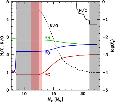
Figure 7: Profile of the CNO abundances through the stellar envelope, as well as the profile of N/C and N/O ratios for the rotating $25\,M_{\odot}$ when it reaches for the first time the RSG branch ($\log(T_{\rm eff})\la 3.6$). The x-axis is the Lagrangian mass coordinate, and we show only the region above the convective core ($7.80\,M_{\odot}$). The light grey zones correspond to convective layers. The light red zone corresponds to the region with $0.6<M_{\rm core}/M_{r}<0.7$, corresponding to minimum values of the ratio of the core mass to the total mass that is required to have a blue loop.

Table 3 shows surface helium abundance and ratios of CNO elements (mass fraction) for BSG models (with rotational mixing) at $\log T_{\rm eff}\approx 4.0$ before and after the RSG stage. Most of the stars listed in Table 2 do not have measured N/C and N/O ratios and thus cannot be used to test the above predictions. There are however two stars Rigel and Deneb for which such data exist. Przybilla et al. (2010) lists (Y, N/C,N/O)= (0.32, 3.4, 0.65) for Deneb and (0.37, 2.0,0.46) for Rigel. These numbers are rather consistent with models before the RSG stage, in contradiction with our conclusion that they should rather be stars having evolved through a RSG stage.

So we are left here with a puzzle: pulsation properties tell us that these two stars should be BSG evolved from a RSG stage, while surface abundances indicate that they should be BSG having directly evolved from the MS phase. In other words, in order to have the excited modes compatible with the observations of Deneb and Rigel, a high $L/M$ ratio is needed, which, in turn, implies strongly changed N/C and N/O ratios which are not observed.

So we are left with a real puzzle here. At this point we can simply mention three directions which may help in resolving this discrepancy:

1) Are we sure that all the frequency measured correspond to pulsation process? For instance, some variations could be due to some other type of instabilities at the surface. In this case, the vertical lines associated to Rigel and Deneb in Fig. 5 representing the observed pulsation period ranges might be reduced and be compatible with stars on their first crossing.

2) It would be extremely interesting to obtain accurate measurements of the N/C and N/O ratios at the surface of the stars listed in Table 2 other than Rigel and Deneb to see whether the case of Deneb and Rigel are representative of all these stars or not. In particular, measurements of surface CNO abundances of the two radial pulsators A10 and D12 in NGC 300 are most interesting.

3) Recently some authors (Davies et al., 2013) find that the RSG have significantly higher effective temperatures and are hence more compact for a given luminosity. From another perspective, Dessart & Hillier (2011) find that to reproduce the light curve of type II-P supernovae, the RSG progenitor should be more compact than predicted by current models. The effective temperature of the RSG stars depends on the physics of the convective envelope. For instance, depending whether turbulent pressure is accounted for or not and how the mixing length is computed, much bluer positions for the RSG stars can be obtained (see e.g. Fig. 9 in Maeder & Meynet, 1987). One can wonder whether more compact RSG stars would need to lose as much mass as larger RSG stars to evolve to the blue part of the HR diagram. Would the blue supergiants resulting from the evolution of more compact RSG stars present the same chemical enrichments as those presented by the current models? We shall investigate these questions in a forthcoming work.

5 Conclusions

We have studied the pulsation properties of BSG models. In the effective temperature range between the blue edge of the cepheid instability strip and the red-edge of the $\beta$ Cephei instability range, where many $\alpha$ Cygni variables reside, radial (and most of nonradial) pulsations are excited only in the models evolving on a blue-loop after losing significant mass in the RSG stage. The observed quasi periods of $\alpha$ Cygni variables are found to be roughly consistent with periods predicted from these models in most cases. This indicates that the $\alpha$ Cygni variables are mainly He-burning stars on the blue-loop.

However, it is found that the abundance ratios N/C and N/O on the surface seem too high compared with spectroscopic results. Further spectroscopic and photometric investigations for BSGs are needed as well as theoretical searches for missing physics in our models.

Furthermore, It would be interesting to explore the circumstellar environments of those stars that are believed to have evolved from a RSG stage. Some of those stars may still have observable relics of the slow and dusty winds that they emitted when they were red supergiants.

Appendix A Rotation profiles in BSG models

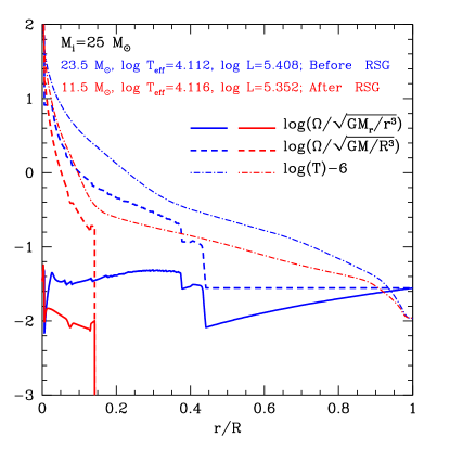
Figure 8: Rotation and temperature profiles as functions of the fractional radius, $r/R$, in two BSG models. The two models started with $M_{\rm i}=25M_{\odot}$, and have similar effective temperatures, but are on different evolutionary stages. Blue lines are used for the model evolving toward the red supergiant stage, while red lines are for the model evolving on the blue-loop after the red supergiant stage. The rotation frequency, $\Omega(r)$, is normalized in two different ways; by local gravity frequency $\sqrt{GM_{r}/r^{3}}$ (solid lines), and by the global one $\sqrt{GM/R^{3}}$ (dashed lines).

For models including rotation effects, the initial rotation speed is assumed to be 40% of the critical rate at the surface of the zero-age main-sequence models. Although the rotation speed is considerable during the main-sequence stage, it decreases significantly in the envelopes of supergiant models because of the expansion and mass loss. Fig. 8 shows runs of angular frequency of rotation in two BSG models having similar effective temperatures; one (blue lines) is evolving toward the red supergiant stage and one (red lines) evolving on the blue loop after the red supergiant stage. In this figure, each rotation profile, $\Omega(r)$, is normalized by two different quantities; $\sqrt{GM_{r}/r^{3}}$ (solid line) and $\sqrt{GM/R^{3}}$ (dashed line). The solid lines indicate that in both models the mechanical effect of rotation on the stellar structure is small because it is much smaller than the local gravity throughout the interior; i.e., $\Omega(r)/\sqrt{GM_{r}/r^{3}}\ll 1$.

The dashed lines in Fig. 8 indicate rotation frequency itself normalized by the global parameters in the same way as the normalized pulsation frequency shown, e.g., in Fig. 3. Although the rotation frequency is very high in the core of a supergiant, in the envelope it is much smaller than the pulsation frequencies; $\ga 1$ for radial pulsations (Fig. 3) and $\ga 0.3$ for nonradial oscillatory convection modes in the same normalization. Since these pulsations are well confined to the stellar envelope ($\log T<6$, see Figs. 4 and 6), rotation hardly influence the pulsation property in these supergiant models. This justifies our pulsation analyses without including the effect of rotation.

References

- Aerts et al. (2006) Aerts C., Marchenko S.V., Matthews J.M., Kuschnig R., Guenther D.B., Moffat A.F.J., Rucinski S.M., Sasselov D., Walker G.A.H., Weiss W.W., 2006, ApJ, 642, 470
- Aerts et al. (2010a) Aerts C., Christensen-Dalsgaard J., Kurtz D., 2010a, Asteroseismology (Springer)
- Aerts et al. (2010b) Aerts C., Lefever K., Baglin A., Degroote P., Oreiro R., Vučković M., Smolders K., Acke B., Verhoelst T., Desmet M., Godart M., Noels A., Dupret M.-A., Auvergne M., Baudin F., Catala C., Michel E., Samadi R., 2010b, A&A, 513, L11
- Asplund, Grevesse, & Sauval (2005) Asplund M., Grevesse N., Sauval A.J., 2005, in Cosmic Abundances as Records of Stellar Evolution and Nucleosynthesis, ed. T.G. Barnes, III & F.N. Bash (San Francisco: ASP), PASP, 336, 25
- Bresolin et al. (2004) Bresolin F., Pietrzyński G., Gieren W., Kudritzki R.-P., Przybilla N., Fouqué P., 2004, ApJ, 600, 182
- Cox (1974) Cox, J.P., 1974, Rep.Prog.Phys., 37, 563
- Cunha, Hubeny, & Lanz (2006) Cunha K., Hubeny I., Lanz T., 2006, ApJ, 647, L143
- Danchi et al. (1994) Danchi W. C., Bester M., Degiacomi C. G., Greenhill L. J., Townes C. H., 1994, AJ, 107, 1469
- Davies et al. (2013) Davies B., Kudritzki R.-P., Plez B., Trager S., Lançon A. Gazak Z., Bergemann M., Evans C., Chiavassa A., 2013, ApJ, 767, 3
- (10) de Jager C., Nieuwenhuijzen H., van der Hucht K. A., 1988, A&AS, 72, 259
- De Ridder et al. (2004) De Ridder J., Telting J.H., Balona L.A., Handler G., Briquet M., Daszyńska-Daszkiewicz J., Lefever K., Korn A.J., Heiter U., Aerts C., 2004, MNRAS, 351, 324
- Dessart & Hillier (2011) Dessart L., Hillier D.J., 2011, MNRAS, 410, 1739
- Dupret et al. (2004) Dupret M.-A., Thoul A., Scuflaire R., Daszyńska-Daszkiewicz J., Aerts C., Bourge P.-O., Waelkens C., Noels A., 2004, A&A, 415, 251
- Dziembowski & Sławińska (2005) Dziembowski W.A., Sławińska J., 2005, AcA, 55, 195
- Ekström et al. (2012) Ekström S., Georgy C., Eggenberger P., Meynet G., Mowlavi N., Wyttenbach A., Granada A., Decressin T., Hirschi R., Frischknecht U., Charbonnel C., Maeder A., 2012, A&A, 537, A146
- Eggenberger et al. (2002) Eggenberger P., Meynet G., Maeder A., 2002, A&A, 386, 576
- Eldridge et al. (2013) Eldridge J.J., Fraser M., Smartt S.J., Maund J.R., R. Crockett R.M., 2013, arXiv, 1301.1975
- Firnstein & Pryzbilla (2012) Firnstein M., Pryzbilla N., 2012, A&A, 543, A80
- Fokin et al. (2004) Fokin A., Mathias Ph., Chapellier E., Gillet D., Nardetto N., 2004, A&A, 426, 687
- Fraser et al. (2010) Fraser M., Dufton P.L., Hunter I., Ryans R.S.I., 2010, MNRAS, 404, 1306
- Gautschy (1992) Gautschy A., 1992, MNRAS, 259, 82
- Gautschy (2009) Gautschy A., 2009, MNRAS, 498, 273
- Gautschy & Glatzel (1990) Gautschy A., Glatzel W., 1990, MNRAS, 245, 597
- Georgy (2012) Georgy C., 2012, A&A, 538, L8
- Georgy et al. (2012) Georgy C., Ekström S., Meynet G., Massey P., Levesque E.M., Hirschi R., Eggenberger P., Maeder A., 2012, A&A, 542, A29
- Giannone (1967) Giannone P., 1967, Zeitschrift für Astrophysik, 65, 226
- Glatzel (1994) Glatzel W., 1994, MNRAS, 271, 66
- Glatzel & Mehren (1996) Glatzel W., Mehren S., 1996, MNRAS, 282, 1470
- Godart et al. (2009) Godart M., Noels A., Dupret M.-A., Lebreton Y., 2009, MNRAS, 396, 1833
- Grevesse & Noels (1993) Grevesse N., Noels A., 1993, in Origin and evolution of the elements, ed. N. Prantzos, E. Vangioni-Flam, & M. Casse, 15
- Handler et al. (2003) Handler G., Shobbrook R.R., Vuthela F.F., Balona L.A., Rodler F., Tshenye T., 2003, MNRAS, 341, 1005
- Handler et al. (2006) Handler G., Jerzykiewicz M., Rodríguez E., Uytterhoeven K., Amado P.J., Dorokhova T.N., Dorokhov N.I., Poretti E., Sareyan J.-P., Parrao L., Lorenz D., Zsuffa D., Drummond R., Daszyńska-Daszkiewicz J., Verhoelst T., De Ridder J., Acke B., Bourge P.-O., Movchan A.I., Garrido R., M. Paparó M., Sahin T., Antoci V., Udovichenko S.N., Csorba K., Crowe R., Berkey B., Stewart S., Terry D., Mkrtichian D.E., Aerts C., 2006, MNRAS, 365, 327
- Hunter et al. (2009) Hunter I., Brott I., Langer N., Lennon D.J., Dufton P.L., Howarth I.D., Ryans R.S.I., Trundle C., Evans C.J., de Koter A., Smartt S.J., 2009, A&A, 496, 841
- Kaltcheva & Scorcio (2010) Kaltcheva N., Scorcio M., 2010, A&A, 514, 59
- Kaufer et al. (1996) Kaufer A., Stahl O., Wolf B., Gäng Th., Gummersbach C.A., Kovács J., Mandel H., Szeifert Th., 1996, A&A, 305, 887
- Kaufer et al. (1997) Kaufer A., Stahl O., Wolf B., Fullerton A.W., Gäng Th., Gummersbach C.A., Jankovics I., Kovács J., Mandel H., Peitz J., Rivinius Th., Szeifert Th., 1997, A&A, 320, 273
- Kudritzki et al. (1999) Kudritzki R.-P., Puls J., Lennon D.J., Venn K.A., Reetz J., Najarro F., McCarthy J.K., Herrero A. 1999, A&A, 350, 970
- Kudritzki et al. (2008) Kudritzki R.-P., Urbaneja M.A., Bresolin F., Przybilla N., Gieren W., Pietrzyński G., 2008, ApJ, 681, 269
- Langer & Maeder (1995) Langer N., Maeder A., 1995, A&A, 295, 685
- Lefever et al. (2007) Lefever K., Puls J., Aerts C., 2007, A&A, 463, 1093
- Leitherer & Wolf (1984) Leitherer C., Wolf B., 1984, A&A, 132, 151
- Markova & Puls (2008) Markova M., Puls J., 2008, A&A, 478, 823
- Maeder & Meynet (1987) Maeder A., Meynet, G., 1987, A&A, 182, 243
- Mazumdar et al. (2006) Mazumdar A., Briquet M., Desmet M., Aerts C., 2006, A&A, 459, 589
- Meylan & Maeder (1983) Meylan G., Maeder A., 1983, A&A, 124, 84
- Moravveji et al. (2012a) Moravveji E., Guinan E.F., Shultz M., Williamson M.H., Moya A., 2012a, ApJ, 747, 108
- Moravveji et al. (2012b) Moravveji E., Moya A., Guinan E.F., 2012b, ApJ, 749, 74
- Percy et al. (2008) Percy J.R., Palaniappan R., Seneviratne R., 2008, PASP, 120, 311
- Przybilla et al. (2006) Przybilla N., Butler K., Becker S.R., Kudritzki R.P., 2006, A&A, 445, 1099
- Przybilla et al. (2010) Przybilla N., Firnstein M., Nieva M.F., Meynet G., Maeder A., 2010, A&A, 517, A38
- Richardson et al. (2011) Richardson N.D., Morrison N.D., Kryukova E.E., Adelman S.J., 2011, AJ, 141, 17
- Saio (2009) Saio H., 2009, CoAst, 158, 245
- Saio (2011) Saio H., 2011, MNRAS, 412, 1814
- Saio et al. (1998) Saio H., Baker N.H., & Gautschy A., 1998, MNRAS, 294, 622
- Saio & Cox (1980) Saio H., Cox J.P., 1980, ApJ, 236, 549
- Saio et al. (2006) Saio H., Kuschnig R., Gautschy A., Cameron C., Walker G. A. H., Matthews J. M., Guenther D. B., Moffat A. F. J., Rucinski S. M., Sasselov D., Weiss W. W., 2006, ApJ, 650, 1111
- Saio, Winget, & Robinson (1983) Saio H., Winget D.E., Robinson E.L., 1983, ApJ, 265, 982
- Salasnich et al. (1999) Salasnich B., Bressan A., Chiosi, C., 1999, A&A, 342, 131
- Schiller & Przybilla (2008) Schiller F., Przybilla N. 2008, A&A, 479, 849
- Shibahashi & Osaki (1981) Shibahashi H., Osaki Y., 1981, PASJ, 33, 427
- Shobbrook et al. (2006) Shobbrook R.R., Handler G., Lorenz D., Mogorosi D., 2006, MNRAS, 369, 171
- Smith, Hinkle, & Ryde (2009) Smith N., Hinkle K. H., Ryde N., 2009, AJ, 137, 3558
- Sterken (1977) Sterken C., 1977, A&A, 57, 361
- Sterken et al. (1999) Sterken C., Arentoft T., Duerbeck H.W., Brogt E., 1999, A&A, 349, 532
- Takeda & Takada-Hidai (2000) Takeda Y., Takada-Hidai M., 2000, PASJ, 52, 113
- Thoul et al. (2003) Thoul A., Aerts C., Dupret M. A., Scuflaire R., Korotin S. A., Egorova I. A., Andrievsky S. M., Lehmann H., Briquet M., De Ridder J., Noels A., 2003, A&A, 406, 287
- Unno et al. (1989) Unno W., Osaki Y., Ando H., Saio H., Shibahashi H., 1989, Nonradial Oscillations of Stars, Univ. of Tokyo Press, Tokyo
- Vanbeveren et al. (1998) Vanbeveren D., De Donder E., van Bever J., van Rensbergen W., De Loore C., 1998, NewA, 3, 447
- Vanbeveren et al. (2012) Vanbeveren C., Mennekens N., Van Rensbergen W., De Loore C., 2012, arXiv, 1212.4285
- van Leeuwen, et al. (1998) van Leeuwen F., van Genderen A.M., Zegelaar I., 1998, A&AS,128, 117
- van Loon et al. (2005) van Loon J. T., Cioni M.-R. L., Zijlstra A. A., Loup C., 2005, A&A, 438, 273
- Yoon & Cantiello (2010) Yoon S.-C., Cantiello M., 2010, ApJ, 717, L62
- Yoon et al. (2012) Yoon S.-C., Gräfener G., Vink J.S., Kozyreva A., Izzard R.G., 2012, A&A, 544, L11