Long-Range Interaction of Singlet-Triplet Qubits via Ferromagnets

Abstract

We propose a mechanism of a long-range coherent interaction between two singlet-triplet qubits dipolarly coupled to a dogbone-shaped ferromagnet. An effective qubit-qubit interaction Hamiltonian is derived and the coupling strength is estimated. Furthermore we derive the effective coupling between two spin-$1/2$ qubits that are coupled via dipolar interaction to the ferromagnet and that lie at arbitrary positions and deduce the optimal positioning. We consider hybrid systems consisting of spin-$1/2$ and ST qubits and derive the effective Hamiltonian for this case. We then show that operation times vary between 1MHz and 100MHz and give explicit estimates for GaAs, Silicon, and NV-center based spin qubits. Finally, we explicitly construct the required sequences to implement a CNOT gate. The resulting quantum computing architecture retains all the single qubit gates and measurement aspects of earlier approaches, but allows qubit spacing at distances of order 1$\,\mu$m for two-qubit gates, achievable with current semiconductor technology.

I Introduction

At the heart of quantum computation lies the ability to generate, measure, and control entanglement between qubits. This is a difficult task because the qubit state is rapidly destroyed by the coupling to the environment it is living in. Hence, a qubit system appropriate for quantum computing must be sufficiently large for it to be controllable by experimentalist but must contain as few degrees of freedom as possible that couple to the environment. One of the most successful candidates for encoding a qubit is an electron spin localized in a semiconductor quantum dot, gate-defined or self-assembled, or a singlet-triplet qubit with two electrons in a double quantum well. Kloeffel and Loss (2013); Levy (2002) These natural two-level systems are very long-lived (relaxation time $T_{1}\sim 1s$, see Ref. Amasha et al., 2008, and decoherence time $T_{2}>200\mu s$, see Ref. Bluhm et al., 2011), they can be controlled efficiently by both electric and magnetic fields, Petta et al. (2005); Koppens et al. (2008); Brunner et al. (2011) and, eventually, may be scaled into a large network. It has been experimentally demonstrated that qubit-qubit couplings can be generated and controlled efficiently for these systems. Shulman et al. (2012) However the separation between the quantum dots needs to be small ($\sim 100nm$) and this renders their scaling to a very large number of qubits a perplexed task. Indeed, the physical implementation of quantum dot networks requires some space between the qubits for the different physical auxiliary components (metallic gates, etc.). It is therefore important to find a way to couple qubits over sufficiently large distances (micrometer scale) to satisfy the space constraint.

Another type of promising two-level systems are silicon-based spin qubits. They are composed of nuclear (electron) spin of phosphorus atoms in a silicon nanostructure. It has recently been shown that very long decoherence times $T_{2}\approx 60ms$ Pla et al. (2013) ($T_{2}\approx 200\mu s$ Pla et al. (2012)) and high fidelity single qubit gates and readout are experimentally achievable. However, the realization of such qubits is subject to randomness of the phosphorus atom position in silicon. Hence, their location is a priori unknown. If two randomly chosen qubits are well-separated from each other, they will hardly interact. On the contrary, when they lie close to each other, it will be difficult to turn-off the interaction since they will not be isolated from each other. In this context it is especially important to be able to couple two qubits over relatively large distances by putting some coupler between them. The aim of our work is to show that this is possible by putting a micrometer-sized ferromagnet between the qubits. We point out that our analysis is general and does not depend on the precise nature of the qubits that need to be coupled as long as they interact dipolarly with the ferromagnet. Hence we think that our analysis is applicable to a variety of other spin qubits systems such as N-V centers in diamond. Dobrovitski et al. (2013)

There have been various other propsals over the last years in order to couple spin qubits over large distances. Among them we mention here coupling through a superconductor, Choi et al. (2000); Leijnse and Flensberg (2013) microwave cavities, Trif et al. (2008); Wallraff et al. (2004) two-dimensional electron gas (RKKY), Rikitake and Imamura (2005) and floating gates. Flensberg and Marcus (2010); Trifunovic et al. (2012); Flindt et al. (2006); Trif et al. (2007)

In this work, we propose and study a system that allows for coherent coupling between ST-qubits as well as between spin-$1/2$ qubits over distances of about one micrometer. The coupler is a ferromagnet composed of two disks separated by a thin quasi-1D region, see Fig. 1. The qubits are coupled to the ferromagnet via dipolar interaction and they are positioned in the vicinity of each disk. The relevant quantity of the coupler, describing the effective coupling between the distant qubits, is its spin-spin susceptibility—a slowly spatially decaying real part of the susceptibility is required in order to mediate interactions over long distances. Additionally, in order to have coherent coupling, the imaginary part of the susceptibility should be sufficiently small. The spatial decay of the spin susceptibility depends strongly on the dimensionality of the ferromagnet—it is longer ranged in lower dimensions. The dogbone shape of the coupler considered here is thus optimal: it allows for strong coupling to the ferromagnet because many spins of each disk lie close to the qubits, while the coherent interaction between them is mediated by the quasi-1D channel. Actually the statement on the optimal shape of the coupler is quite general if we consider a realistic interaction between the qubit and the coupler, i.e., a Coulomb Trifunovic et al. (2012) or a dipolar one as herein.

Likewise, we derive a Hamiltonian for the effective interaction between the distant qubits positioned arbitrarily with respect to each disk of the dogbone and determine what is the optimal position for the coupling to be strongest. For ST-qubit the optimal coupling is obtain if one quantum well is positioned directly below the disk center and the other one below the edge of the disk, while for the spin-$1/2$ qubits it is optimal to place them at the edge of the disk. Similar conclusions about the optimal positioning of the qubits with respect to the coupler were previously obtained for the case of electrostatic interaction. Trifunovic et al. (2012)

In the most favorable scenarios described above the coupling strength of $10^{-2}\mu{\rm eV}$ are achieved for ST-qubits as well as for spin-$1/2$ qubits. The clock speed for such coupling schemes thus varies between 1MHz and 100MHz. We summarize in Tables 1 and 2 of Section VIII the coupling strengths and corresponding operation times achievable with our scheme.

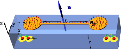
Figure 1: Model system consisting of two identical double-QDs in the $xy$-plane and the dogbone-shaped coupler. The dogbone coupler consists of two ferromagnetic disks of radius $R_{0}$ connected by a thin ferromagnetic wire of length $L$. Each double-QD can accommodate one (two) electrons, defining the spin-$1/2$ (ST-) qubit. Absence of tunneling between the separate double-QD is assumed. Here $R_{\rm L}$ ($R_{\rm R}$) is the in-plane distance between the left (right) well and the corresponding disk center, while $h$ is vertical distance between the QD and the gate. The red arrow on top of the ferromagnet denote the orientation of its magnetization which is assumed to be monodomain.

In order to be useful for quantum computation, one needs to be able to turn on and off the coupling between the qubits. This is efficiently achieved by putting the qubit splitting off-resonance with the internal splitting of the ferromagnet. As we argue below, a modification in the qubit splitting of about one percent of $\Delta_{F}$ is enough to interrupt the interaction between the qubits. Finally we derive for both qubit systems the sequence to implement the entangling gates CNOT (and iSWAP) that can be achieved with a gate fidelity exceeding 99.9%. The additional decoherence effects induced solely by the coupling to the ferromagnet are negligible for sufficiently low temperatures ($T\lesssim 0.1K$).Trifunovic et al. (2013) We then obtain error thresholds—defined as the ratio between the two-qubit gate operation time to the decoherence time—of about $10^{-4}$ for ST-qubits as well as for spin-1/2 qubits and this is good enough to implement the surface code error correction in such setups. This quantum computing architecture thus retains all the single qubit gates and measurement aspects of earlier approaches, but allows qubit spacing at distances of order 1$\,\mu$m for two-qubit gates, achievable with current semiconductor technology.

The paper is organized as follows. In Sections II and III.1 we introduce the ferromagnet and ST-qubit Hamiltonian, respectively. In Sec. III.2 we derive the effective dipolar coupling between the ST-qubit and the ferromagnet. In Sec. III.3 we make use of a perturbative Scrhieffer-Wolff transformation to derive the effective coupling between the two ST-qubits that is mediated by the ferromagnet. We determine the optimal position of the qubits relative to the disks of the dogbone. In Sec. III.4 we construct the sequence to implement the CNOT (and iSWAP) gate and calculate the corresponding fidelity of the sequence. In Sec. IV we study the coupling between two spin-$1/2$ qubits positioned at arbitrary location with respect to the adjacent disk of the dogbone-shaped ferromagnet. We derive an effective Hamiltonian for the interaction of the two spin-$1/2$ qubits mediated by the ferromagnet and determine the optimal position of the qubits. In Sec. IV.1 we derive the sequence to implement the CNOT (and iSWAP) gate. In Sec. V, we show that spin-$1/2$ and ST qubits can be cross-coupled leading to hybrid qubits and we derive the effective Hamiltonian for this case. In Sec. VI, we discuss the range of validity of our effective theory. The on/off switching mechanisms of the qubit-qubit coupling are discussed in Sec. VII. In Sec. VIII, we present a table with the effective coupling strengths and operation times achievable in our setup for four experimentally relevant systems, namely GaAs spin-$1/2$ quantum dots, GaAs singlet-triplet quantum dots, silicon-based qubits, and N-V centers. Finally, Sec. IX contains our final remarks and the Appendices additional details on the models and derivations.

II Ferromagnet

We denote by $\bm{S}_{\bf r}$ the spins (of size $S$) of the ferromagnet at site ${\bf r}$ on a cubic lattice and $\bm{\sigma}_{i}$ stands for the spin-$1/2$ qubit spins. The ferromagnet Hamiltonian we consider is of the following form

$$H_{F}=-J\sum_{\langle{\bf r},{\bf r^{\prime}}\rangle}{\bm{S}}_{\bf r}\cdot{\bm{S}}_{\bf r^{\prime}}+\Delta_{F}\sum_{{\bf r}}S^{z}_{\bf r},$$ (1)

with $J>0$ and $\Delta_{F}=\mu B$, where $B$ is externally applied magnetic field (see Fig. 1) and $\mu$ is the magnetic moment of the ferromagnet spin. The above Hamiltonian is the three-dimensional (3D) Heisenberg model with the sum restricted to nearest-neighbor sites $\langle{\bf r},{\bf r^{\prime}}\rangle$. The ferromagnet is assumed to be monodomain and below the Curie temperature with the magnetization pointing along the $z$-direction.

We would like to stress at this point that even though herein we analyze a specific model for the ferromagnet (Heisenberg model), all our conclusions rely only on the generic features of the ferromagnet susceptibility, i.e., its long-range nature. Furthermore, the gap in the magnon spectrum can originate also from anisotropy. The presence of the gap is an important feature since it suppresses the fluctuations, albeit the susceptibility is cut-off after some characteristic length given by the gap and the frequency at which the ferromagnet is probed.

III Coupling between ST-qubits

The Hamiltonian we consider is of the following form

$$H=H_{F}+H_{\tau}+H_{I},$$ (2)

where $H_{\tau}$ is Hamiltonian of the two ST-qubits Levy (2002); Klinovaja et al. (2012) and $H_{I}$ is the dipolar coupling between the ferromagnet and the ST-qubits (see below).

III.1 Singlet-Triplet qubit Hamiltonian

A Singlet-Triplet (ST) qubit is a system that consists of two electrons confined in a double quantum well. Herein we assume that the wells are steep enough so that we can consider only one lowest orbital level of each well. Following Ref. Stepanenko et al., 2012, we consider also the spin space of the two electrons and write down the total of six basis states

$$|(2,0)S\rangle =c^{\dagger}_{{\rm L}\uparrow}c^{\dagger}_{{\rm L}\downarrow}|0\rangle,$$

$$|(0,2)S\rangle =c^{\dagger}_{{\rm R}\uparrow}c^{\dagger}_{{\rm R}\downarrow}|0\rangle,$$

$$|(1,1)S\rangle =\frac{1}{\sqrt{2}}\left(c^{\dagger}_{{\rm L}\uparrow}c^{\dagger}_{{\rm R}\downarrow}-c^{\dagger}_{{\rm L}\downarrow}c^{\dagger}_{{\rm R}\uparrow}\right)|0\rangle,$$

$$|T_{+}\rangle =c^{\dagger}_{{\rm L}\uparrow}c^{\dagger}_{{\rm R}\uparrow}|0\rangle,$$ (3)

$$|T_{0}\rangle =\frac{1}{\sqrt{2}}\left(c^{\dagger}_{{\rm L}\uparrow}c^{\dagger}_{{\rm R}\downarrow}+c^{\dagger}_{{\rm L}\downarrow}c^{\dagger}_{{\rm R}\uparrow}\right)|0\rangle,$$

$$|T_{-}\rangle =c^{\dagger}_{{\rm L}\downarrow}c^{\dagger}_{{\rm R}\downarrow}|0\rangle,$$

where $c^{\dagger}_{\rm L}$ ($c^{\dagger}_{\rm R}$) creates an electron in the Wannier state $\Phi_{\rm L}$ ($\Phi_{\rm R}$). The Wannier states are $\Phi_{\rm\rm L,R}=\frac{1}{\sqrt{1-2sg+g^{2}}}\left(\varphi_{\rm 1,2}-g\varphi_{\rm 2,1}\right)$, where $s=\langle\varphi_{\rm 1}|\varphi_{\rm 2}\rangle=\exp[-\left(a/a_{\rm B}\right)^{2}]$ is the overlap of the harmonic oscillator ground state wave functions of the two wells, $a_{\rm B}=\sqrt{\hbar/m\omega_{0}}$ is the Bohr radius of a single quantum dot, $\hbar\omega_{0}$ is the single-particle level spacing, and $2a=l$ is the interdot distance. The mixing factor of the Wannier states is $g=({1-\sqrt{1-s^{2}}})/{s}$. Using these six basis states we can represent the Hamiltonian of the ST-qubits

$$H_{0}=\left(\begin{array}[]{cc}H_{\rm SS}&0\\ 0&H_{\rm TT,0}\end{array}\right).$$ (4)

In writing the above equation we have neglected the spin-orbit interaction (SOI), thus there are no matrix elements coupling the singlet and triplet blocks. The effect of SOI in ST-qubit was studied in Ref. Stepanenko et al., 2012 and no major influence on the qubit spectra was found.

The two qubit states are $\left|\mbox{$T_{0}$}\right\rangle$ and, in the absence of SOI, the linear combination of the singlet states $\left|\mbox{$S$}\right\rangle=\alpha\left|\mbox{$(2,0)S$}\right\rangle+\beta\left|\mbox{$(1,1)S$}\right\rangle+\gamma\left|\mbox{$(0,2)S$}\right\rangle$, where the coefficients $\alpha,\beta,\gamma$ depend on the detuning $\varepsilon$ between the two quantum wells. In particular, when $\varepsilon=0$ we have $\left|\mbox{$S$}\right\rangle=\left|\mbox{$(1,1)S$}\right\rangle$. In what follows, we always consider Hamiltonians only in the qubit subspace, thus the Hamiltonian of two ST-qubits reads

$$H_{\tau}=-\frac{\Delta}{2}\sum_{i=1,2}\tau_{i}^{z},$$ (5)

where $\tau^{x,y,z}$ are the Pauli matrices acting in the space spanned by vectors $\{\left|\mbox{$S$}\right\rangle,\left|\mbox{$T_{0}$}\right\rangle\}$ and $\Delta$ is the ST-qubit splitting.

III.2 Dipolar coupling to ST-qubit

In this section we derive the dipolar coupling between the ferromagnet and the ST-qubit. To this end we first project the Zeeman coupling to the ST-qubit system on the two-dimensional qubit subspace

$$H_{\rm Z}=g^{*}\mu_{B}\left(\bm{B}_{\rm L}\cdot\bm{S}_{\rm L}+\bm{B}_{\rm R}\cdot\bm{S}_{\rm R}\right)\,,$$ (6)

where $\bm{B}_{\rm L}$ ($\bm{B}_{\rm R}$) is the magnetic field in the left (right) quantum well, $S_{\rm L,R}^{i}=(\sigma^{i})_{ss^{\prime}}c^{\dagger}_{{\rm L,R},s}c_{{\rm L,R},s^{\prime}}$ and $g^{*}$ is the effective Landé factor. After projecting on the qubit space we obtain

$$H_{\rm Z}=g^{*}\mu_{B}(B_{\rm L}^{z}-B_{\rm R}^{z})\tau^{x}.$$ (7)

With this result we are ready to write down the ferromagnet/ST-qubit interaction Hamiltonian

$$H_{I}=\sum_{i=1,2}g^{*}\mu_{0}\mu_{B}\left(\hat{B}_{\rm L}^{z}(i)-\hat{B}_{\rm R}^{z}(i)\right)\tau_{i}^{x},$$ (8)

where index $i$ enumerates ST-qubits, and the magnetic field from the ferromagnet can be express through the integral over the ferromagnet

$$\hat{B}_{\rm L,R}^{z}(i)= \frac{\mu_{0}\mu}{4\pi a^{3}}\int d\bm{r}(i)_{\rm L,R}\frac{1}{r(i)_{\rm L,R}^{3}}\times$$ (9)

$$\left(S^{z}_{\bm{r}(i)_{\rm L,R}}-\frac{3(\bm{S}_{\bm{r}(i)_{\rm L,R}}\cdot\bm{r}(i)_{\rm L,R})r(i)_{\rm L,R}^{z}}{r(i)_{\rm L,R}^{2}}\right),$$

where the coordinate system for $\bm{r}(i)_{\rm L}$ ($\bm{r}(i)_{\rm R}$) is positioned in left (right) quantum well of the $i$-th qubit.

III.3 Effective coupling between two ST-qubits

Given the total Hamitonian, Eq. (2), we can easily derive the effective qubit-qubit coupling with help of Schrieffer-Wolff transformation

$$H_{\rm eff}=H_{\tau}-\lim_{\nu\rightarrow 0^{+}}\frac{i}{2}\int_{0}^{\infty}dte^{-\nu t}\left[H_{I}(t),H_{I}\right],$$ (10)

with $H_{I}(t)=e^{iH_{\tau}t}H_{I}e^{-iH_{\tau}t}$.

We assume that the radius of the two disks is much smaller than the distance between their centers ($R_{0}\ll L$). Within this assumption we can take for the susceptibility between two points at opposite disks the same as the 1D susceptibility. Next we take only on-resonance susceptibility and make use of the expression $\tau^{x}(\Delta)=\frac{1}{2}(\tau^{x}+i\tau^{y})$, where $\tau^{x}(\omega)$ is the Fourier transform of $\tau^{x}(t)=e^{iH_{\tau}t}\tau^{x}e^{-iH_{\tau}t}$. We define the transverse susceptibility in the standard way

$$\chi_{\perp}(\omega,{\bf r}_{i}-{\bf r}_{j})=-i\lim\limits_{\eta\rightarrow 0^{+}}\int_{0}^{\infty}dte^{(-i\omega-\eta)t}[S_{{\bf r}_{i}}^{+}(t),S_{{\bf r}_{j}}^{-}].$$ (11)

The longitudinal susceptibility, defined via

$$\chi_{\parallel}(\omega,{\bf r}_{i}-{\bf r}_{j})=-i\lim\limits_{\eta\rightarrow 0^{+}}\int_{0}^{\infty}dte^{(-i\omega-\eta)t}[S_{{\bf r}_{i}}^{z}(t),S_{{\bf r}_{j}}^{z}],$$ (12)

can be neglected compared to the transverse one because the former is smaller by a factor $1/S$ and is proportional to the magnon occupation number, see Eq. 70. Therefore the longitudinal susceptibility vanishes at zero temperature, while the is not the case for the transverse susceptibility. We arrive finally at the following expression

$$H_{\rm eff}=H_{\tau}+\frac{9}{4}\mathcal{B}\chi^{\rm 1D}_{\perp}(\Delta,L)\tau_{1}^{x}\tau^{x}_{2},$$ (13)

where $\mathcal{B}=(\mu_{0}\mu)^{2}(g^{*}\mu_{B})^{2}(A_{L}^{1}-A_{R}^{1})(A_{L}^{2}-A_{R}^{2})/16\pi^{2}a^{6}$, $\chi_{\perp}^{\rm 1D}$ is given in Eq. (65) and

$$A_{\rm L,R}^{i}=\int d\bm{r}(i)_{\rm L,R}\frac{r(i)^{-}_{\rm L,R}r(i)_{\rm L,R}^{z}}{r(i)_{\rm L,R}^{5}}.$$ (14)

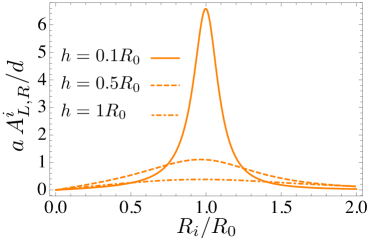
Figure 2: Plot of $aA_{L,R}^{i}/d$ defined through Eq. (14) as function of $R_{i}/R_{0}$ for different values of $h$. We see that the value of $aA_{L,R}^{i}/d$ is bigger when the ST-qubit is closer to the disk of the dogbone as expected. Furthermore, by placing the right dot at distance $R_{0}$ of the disk axis and the left dot on the disk axis, we obtain the strongest value for the effective coupling between the two ST-qubits, see Eq. (13).

Assuming the dogbone shape of the ferromagnet in the above integral and integration only over the adjacent disk, we obtain

$$A_{\rm L,R}^{i}=\frac{2ihd}{a}\frac{2R_{\rm L,R}^{i}R_{0}\left(F(\mathrm{acsc}({w_{\rm L,R}^{i}}),{w_{\rm L,R}^{i}}^{2})-K({w_{\rm L,R}^{i}}^{2})\right)+{u_{\rm L,R}^{i}}E({w_{\rm L,R}^{i}}^{2})-{u_{\rm L,R}^{i}}E(\mathrm{acsc}({w_{\rm L,R}^{i}}),{w_{\rm L,R}^{i}}^{2})}{3R^{i}_{\rm L,R}\left((R_{\rm L,R}^{i}-R_{0})^{2}+h^{2}\right)\sqrt{(R_{\rm L,R}^{i}+R_{0})^{2}+h^{2}}},$$ (15)

where $R_{0}$ is the disk radius, $R_{\rm L,R}^{i}$ is the distance from the adjacent disk axis to the left or right quantum well of the $i$-th qubit, $\mathrm{acsc}(x)$ is the inverse cosecant; $F(x,y)$, $K(x)$ and $E(x,y)$ are the corresponding elliptic integrals. Furthermore, we introduced the notation $u_{\rm L,R}^{i}={R_{\rm L,R}^{i}}^{2}+R_{0}^{2}+h^{2}$ and $w_{\rm L,R}^{i}=\sqrt{1-\frac{4R_{\rm L,R}^{i}R_{0}}{(R_{\rm L,R}^{i}+R_{0})^{2}+h^{2}}}$, where $h$ is the distance in the $z$-direction between the ST-qubit plane and the adjacent disk bottom and $d$ is the disk thickness, see Fig. 1.

Figure 2 illustrates the dependence of the $A^{i}_{\rm L,R}$ integrals on the position of the quantum wells. Since the coupling constant is given by the difference of this integrals for left and right quantum well, we conclude that the strongest coupling is obtained if one quantum well of the ST-qubit is positioned below the disk center and the other exactly below the edge. Furthermore, when $h\ll R_{0}$ the value of the integral is strongly peaked around $R\sim R_{0}$ and this can be exploited as yet another switching mechanism—moving one quantum well away from the edge of the disk.

III.4 Sequence for CNOT gate

Two qubits interacting via the ferromagnet evolve according to the Hamiltonian $H_{\mathrm{eff}}$, see Eq. (13). The Hamiltonian is therefore the sum of Zeeman terms and qubit-qubit interaction. These terms do not commute, making it difficult to use the evolution to implement standard entangling gates. Nevertheless, since $H_{\tau}$ acts only in the subspace spanned by $\{\left|\mbox{$\uparrow\uparrow$}\right\rangle,\left|\mbox{$\downarrow\downarrow$}\right\rangle\}$ and $\Delta\gg J_{12}=9\mathcal{B}\chi_{\perp}(\Delta)/4$, we can neglect the effect of $H_{\mathrm{eff}}$ in this part of the space and approximate it by its projection in the space spanned by vectors $\{\left|\mbox{$\uparrow\downarrow$}\right\rangle,\left|\mbox{$\downarrow\uparrow$}\right\rangle\}$

$$H^{\prime}_{\mathrm{eff}}=H_{\tau}+J_{12}(\tau_{1}^{x}\tau_{2}^{x}+\tau_{1}^{y}\tau_{2}^{y}).$$ (16)

Within this approximation, the coupling in $H^{\prime}_{\mathrm{eff}}$ and Zeeman terms now commute.

We consider the implementation of the iSWAP gate Imamoglu et al. (1999) $U_{\mathrm{iSWAP}}=e^{-i(\tau_{1}^{x}\tau_{2}^{x}+\tau_{1}^{y}\tau_{2}^{y})3\pi/4}$, which can be used to implement the CNOT gate:

$$U_{\mathrm{iSWAP}}=e^{iH_{\tau}t}e^{-iH^{\prime}_{\mathrm{eff}}t},$$ (17)

where $t=3\pi/(4J_{12})$. When iSWAP is available, the CNOT gate can be constructed in the standard way Tanamoto et al. (2008)

$$U_{\rm CNOT}=e^{-i\frac{\pi}{4}\tau_{1}^{z}}e^{i\frac{\pi}{4}\tau_{2}^{x}}e^{i\frac{\pi}{4}\tau_{2}^{z}}U_{\rm iSWAP}e^{-i\frac{\pi}{4}\tau_{1}^{x}}U_{\rm iSWAP}e^{i\frac{\pi}{4}\tau_{2}^{z}}.$$ (18)

Since $H^{\prime}_{\mathrm{eff}}$ is an approximation of $H_{\mathrm{eff}}$, the above sequence will yield approximate CNOT, $U^{\prime}_{\rm CNOT}$, when used with the full Hamiltonian. The success of the sequences therefore depends on the fidelity of the gates, $F(U^{\prime}_{\rm CNOT})$. Ideally this would be defined using a minimization over all possible states of two qubits. However, to characterize the fidelity of an imperfect CNOT it is sufficient to consider the following four logical states of two qubits Trifunovic et al. (2012, 2013): $\left|\mbox{$+,0$}\right\rangle,\left|\mbox{$+,1$}\right\rangle,\left|\mbox{$-,0$}\right\rangle,$ and $\left|\mbox{$-,1$}\right\rangle$. These are product states which, when acted upon by a perfect CNOT, become the four maximally entangled Bell states $\left|\mbox{$\Phi^{+}$}\right\rangle,\left|\mbox{$\Psi^{+}$}\right\rangle,\left|\mbox{$\Phi^{-}$}\right\rangle,$ and $\left|\mbox{$\Psi^{-}$}\right\rangle$, respectively. As such, the fidelity of an imperfect CNOT may be defined,

$$F(U^{\prime}_{\rm CNOT})=\min_{i\in\{+,-\},j\in\{0,1\}}|\left\langle\mbox{$i,j$}\right|U_{\rm CNOT}^{\dagger}U^{\prime}_{\rm CNOT}\left|\mbox{$i,j$}\right\rangle|^{2}.$$ (19)

The choice of basis used here ensures that $F(U^{\prime}_{\rm CNOT})$ gives a good characterization of the properties of $U^{\prime}_{\rm CNOT}$ in comparison to a perfect CNOT, especially for the required task of generating entanglement. For realistic parameters, with the Zeeman terms two order of magnitude stronger than the qubit-qubit coupling, the above sequence yields fidelity for the CNOT gate of $99.976\%$.

To compare these values to the thresholds found in schemes for quantum computation, we must first note that imperfect CNOT’s in these cases are usually modelled by the perfect implementation of the gate followed by depolarizing noise at a certain probability. It is known that such noisy CNOT’s can be used for quantum computation in the surface code if the depolarizing probability is less than $1.1\%$. Wang et al. (2011) This corresponds to a fidelity, according to the definition above, of $99.17\%$. The fidelities that may be achieved in the schemes proposed here are well above this value and hence, though they do not correspond to the same noise model, we can expect these gates to be equally suitable for fault-tolerant quantum computation.

IV Coupling between spin-$1/2$ qubits

In this section we study the coupling of two spin-$1/2$ quantum dots via interaction with a dog-bone shaped ferromagnet. The Hamiltonian has again the form as in Eq. (2) and we allow for splittings of the spin-$1/2$ qubits both along $x$ and $z$ direction,

$$H_{\sigma}=\frac{\Delta_{x}}{2}\sum_{i=1,2}\sigma_{i}^{x}+\frac{\Delta_{z}}{2}\sum_{i=1,2}\sigma_{i}^{z}\,,$$ (20)

where $\bm{\sigma}_{i}$ are the Pauli operators of the $i^{\text{th}}$ spin-$1/2$ quantum dot. Hamiltonian (20) is a generalized version of the Hamiltonian studied in Ref. Trifunovic et al., 2013 where we considered splitting along $x$ only. We present here a detailed derivation of the effective coupling between two quantum dots located at an arbitrary position with respect to the dogbone shaped ferromagnet, i.e., contrary to Ref. Trifunovic et al., 2013 we do not assume that the quantum dots are positioned at a highly symmetric point but consider the most general case. This allows us to determine the optimal positioning of the qubit in order to achieve the strongest coupling between the qubits.

The dipolar coupling between the ferromagnet and the spin-$1/2$ qubits is given by

$$H_{I}=\sum_{i,{\bf r}}\frac{g^{*}\mu_{0}\mu_{B}\mu}{4\pi r^{3}}\left({\bm{\sigma}}_{i}\cdot{\bf S}_{\bf r}-\frac{3({\bm{\sigma}}_{i}\cdot{\bf r})({\bf S}_{\bf r}\cdot{\bf r})}{r^{2}}\right)\,,$$ (21)

where $\mu_{D}$ is the magnetic moment of the spin-$1/2$ qubit. The explicit expressions for the time evolution of the Pauli operators in Heisenberg picture is

$$\sigma_{i}^{+}(t) = -\frac{1}{\Delta^{2}}(i\Delta\cos(\Delta t/2)-\Delta_{z}\sin(\Delta t/2))^{2}\sigma_{i}^{+}$$

$$-\frac{\Delta_{x}^{2}}{2\Delta^{2}}(\cos(t\Delta)-1)\sigma_{i}^{-}$$

$$+\frac{\Delta_{x}}{\Delta^{2}}(\Delta_{z}-\Delta_{z}\cos(t\Delta)-i\Delta\sin(t\Delta))\sigma_{i}^{z}\,,$$

$$\sigma_{i}^{z}(t) = \frac{\Delta_{x}}{2\Delta^{2}}(\Delta_{z}-\Delta_{z}\cos(t\Delta)-i\Delta\sin(t\Delta))\sigma_{i}^{+}$$ (22)

$$+\frac{\Delta_{x}}{2\Delta^{2}}(\Delta_{z}-\Delta_{z}\cos(t\Delta)+i\Delta\sin(t\Delta))\sigma_{i}^{-}$$

$$+\frac{\Delta_{z}^{2}+\Delta_{x}^{2}\cos(t\Delta)}{\Delta^{2}}\sigma_{i}^{z}\,,$$

where we introduced the notation $\Delta=\sqrt{\Delta_{x}^{2}+\Delta_{z}^{2}}$. We also assume that $\Delta<\Delta_{F}$ such that the susceptibility $\chi_{\perp}(\Delta,\bm{r})$ is purely real—thus the transverse noise is gapped. By replacing the above expressions in Eq. (10), we obtain the effective qubit-qubit coupling

$$H_{\text{eff}} =H_{\sigma}+\frac{(g^{*}\mu_{0}\mu_{B}\mu)^{2}}{16\pi^{2}a^{6}}(\frac{9}{8}A_{1}^{*}A_{2}\chi_{\perp}^{\text{1D}}(\Delta)\sigma_{1}^{z}(\Delta)\sigma_{2}^{z}$$

$$+\frac{3}{16}(3A_{2}C_{1}^{*}\chi_{\perp}^{\text{1D}}(\Delta)-B_{1}A_{2}^{*}\chi_{\perp}^{\text{1D}}(\Delta))\sigma_{1}^{+}(\Delta)\sigma_{2}^{z}$$

$$+\frac{3}{16}(3A_{1}C_{2}^{*}\chi_{\perp}^{\text{1D}}(\Delta)-B_{2}A_{1}^{*}\chi_{\perp}^{\text{1D}}(\Delta))\sigma_{1}^{z}(\Delta)\sigma_{2}^{+}$$

$$+\frac{1}{32}(B_{1}B_{2}\chi_{\perp}^{\text{1D}}(\Delta)+9C_{1}C_{2}^{*}\chi_{\perp}^{\text{1D}}(\Delta))\sigma_{1}^{-}(\Delta)\sigma_{2}^{+}$$

$$-\frac{3}{32}(B_{1}C_{2}\chi_{\perp}^{\text{1D}}(\Delta)+B_{2}C_{1}\chi_{\perp}^{\text{1D}}(\Delta))\sigma_{1}^{-}(\Delta)\sigma_{2}^{-}$$

$$+\text{h.c.})+1\leftrightarrow 2\,,$$ (23)

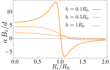
Figure 3: Plot of $aB_{i}/d$ defined in Eq. (26) as function of $R_{i}/R_{0}$ for different values of $h$. The value of the integral increases in general by decreasing the value of $h$.

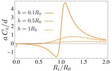
Figure 4: Plot of $aC_{i}/d$ defined in Eq. (25) as function of $R_{i}/R_{0}$ for different values of $h$. The value of the integral is peaked around $R_{i}\sim R_{0}$ and it increases in general by decreasing the value of $h$.

where we have denoted $\chi_{\perp}^{\rm 1D}(\Delta)=\chi_{\perp}^{\rm 1D}(\Delta,L)$ and introduced the following notation for the integrals

$$A_{i} =\int d{\bf r}_{i}\frac{r^{z}_{i}r^{+}_{i}}{r_{i}^{5}}\,,$$ (24)

$$C_{i} =\int d{\bf r}_{i}\frac{(r_{i}^{+})^{2}}{r_{i}^{5}}\,,$$ (25)

$$B_{i} =\int d{\bf r}_{i}\frac{1}{r_{i}^{3}}\left(2-\frac{3r_{i}^{+}r_{i}^{-}}{r_{i}^{2}}\right)\,,$$ (26)

with the coordinate origin for ${\bf r}_{i}$ at the $i$-th qubit and the integration goes over the adjacent disk. We also defined the Fourier transforms of the time evolution of Pauli matrices $\bm{\sigma}(t)=e^{iH_{\sigma}t}\bm{\sigma}e^{-iH_{\sigma}t}$ as

$$\sigma_{i}^{+}(\Delta) = -\frac{1}{\Delta^{2}}\left(-\frac{\Delta^{2}}{4}+\frac{\Delta_{z}\Delta}{2}-\frac{\Delta_{z}^{2}}{4}\right)\sigma_{i}^{+}$$

$$+\frac{\Delta_{x}}{\Delta^{2}}\left(-\frac{\Delta_{z}}{2}+\frac{\Delta}{2}\right)\sigma_{i}^{z}-\frac{\Delta_{x}^{2}}{4\Delta^{2}}\sigma_{i}^{-}\,,$$

and

$$\sigma_{i}^{z}(\Delta) = \frac{\Delta_{x}}{2\Delta^{2}}\left(-\frac{\Delta_{z}}{2}+\frac{\Delta}{2}\right)\sigma_{i}^{+}+\frac{\Delta_{x}}{2\Delta^{2}}\left(-\frac{\Delta_{z}}{2}-\frac{\Delta}{2}\right)\sigma_{i}^{-}$$ (27)

$$+\frac{\Delta_{x}^{2}}{2\Delta^{2}}\sigma_{i}^{z}\,.$$

By assuming a dogbone-shaped ferromagnet and integrating only over the adjacent disk as above, we obtain $A_{i}$ given in Eq. (15) with $R_{L,R}^{i}$ replaced by $R_{i}$ since there is now only one spin-$1/2$ qubit below each disk of the dogbone. The remaining integrals yield the following results

$$B_{i} = -\frac{2d}{3a}\frac{\left(R_{i}^{4}+3R_{i}^{2}\left(h^{2}-R_{0}^{2}\right)+\left(R_{0}^{2}+h^{2}\right)^{2}\right)E\left(1-w_{i}^{2}\right)-\left((R_{i}-R_{0})^{2}+h^{2}\right)\left(R_{i}^{2}+2\left(R_{0}^{2}+h^{2}\right)\right)K\left(1-w_{i}^{2}\right)}{R_{i}^{2}\left((R_{i}-R_{0})^{2}+h^{2}\right)\sqrt{(R_{i}+R_{0})^{2}+h^{2}}}\,,$$

$$C_{i} = \frac{2d}{a}\frac{\left((R_{i}-R_{0})^{2}+h^{2}\right)K\left(1-w_{i}^{2}\right)-2\left(R_{i}^{2}-R_{0}^{2}+h^{2}\right)E\left(1-w_{i}^{2}\right)}{\left((R_{i}-R_{0})^{2}+h^{2}\right)\sqrt{(R_{i}+R_{0})^{2}+h^{2}}}\,,$$ (28)

where $w_{i}=\sqrt{1-\frac{4R_{i}R_{0}}{(R_{i}+R_{0})^{2}+h^{2}}}$, $R_{0}$ is the radius of each disk, $R_{i}$ is the distance of the $i$-th qubit to the adjacent dog bone axis, and $R_{0}$ and $h$ are defined as in Sec. III.3. In deriving Eq. (IV) we took again only ‘on-resonance’ terms into account (i.e. we neglected $\chi_{\perp}^{\text{1D}}(0)$ and $\chi_{\perp}^{\text{1D}}(-\Delta)$). Furthermore we assumed, as above, that the susceptibility between two points on different disks of the dogbone is well approximated by the 1D transverse susceptibility. In the limit where each quantum dot lies on the vertical axis going through the center of each cylinder of the dogbone, the axial symmetry leads to $A_{1}=A_{2}=C_{1}=C_{2}=0$, $B_{1}=B_{2}=B$, and with $\Delta_{z}=0$ we recover the result

$$H_{\text{eff}}=H_{\sigma}+\frac{(g^{*}\mu_{0}\mu_{B}\mu)^{2}}{16\,\pi^{2}a^{6}}\frac{B^{2}}{32}\chi^{\rm 1D}_{\perp}(\Delta)(2\sigma_{1}^{y}\sigma_{2}^{y}+\sigma_{1}^{z}\sigma_{2}^{x}+\sigma_{1}^{x}\sigma_{2}^{z})$$ (29)

derived in Ref. Trifunovic et al., 2013. The analysis carried out herein assumes arbitrary positioning of the qubit and allow us to determine the optimal positioning for the strongest coupling. To this end, we analyze integrals $A_{i},\;B_{i},\;C_{i}$, see Figs. 2-4. It is readily observed that the coupling strength increases as the vertical distance between the qubit and coupler plane, $h$, decreases. Additionally, we observe that the strongest coupling strength is obtained when the qubit is positioned below the edge of the adjacent disk.

The derived coupling is valid for any dogbone-like shape of the ferromagnet, i.e., it is not crucial to assume disk shape.

IV.1 Sequence for CNOT gate

The effective Hamiltonian derived in previous section, Eq. (IV), can be re-expressed in the following form

$$H_{\rm eff}=\frac{(g^{*}\mu_{0}\mu_{B}\mu)^{2}}{16\pi^{2}a^{6}}\chi_{\perp}^{\rm 1D}(\Delta,L)\bm{\sigma}_{1}^{T}\cdot\hat{\mathcal{H}}\cdot\bm{\sigma}_{2}+\frac{1}{2}\bm{\Delta}\cdot(\bm{\sigma}_{1}+\bm{\sigma}_{2}),$$ (30)

with $\bm{\Delta}=(\Delta_{x},0,\Delta_{z})^{T}$ and $\hat{\mathcal{H}}$ being the symmetric matrix with all entries being non-zero. The question now arises how to construct the CNOT gate sequence for such a general Hamiltonian. We tackle this problem by taking first the quantization axis to be along the total magnetic field acting on the two qubits and denote by $\tilde{\bm{\sigma}}_{i}$ Pauli matrix vector with respect to this new quantization axis. The Hamiltonian now reads

$$H_{\rm eff}=\frac{(g^{*}\mu_{0}\mu_{B}\mu)^{2}}{16\pi^{2}a^{6}}\chi_{\perp}^{\rm 1D}(\Delta,L)\,\tilde{\bm{\sigma}}_{1}^{T}\cdot\hat{\tilde{\mathcal{H}}}\cdot\tilde{\bm{\sigma}}_{2}+\frac{1}{2}\Delta(\tilde{\sigma}_{1}^{z}+\tilde{\sigma}_{2}^{z}),$$ (31)

where the components of the matrix $\hat{\tilde{\mathcal{H}}}$ are given in Appendix D.

We proceed further along the lines presented in Sec. III.4, i.e., we project the rotated Hamiltonian, Eq. (31), on the subspace spanned by vectors $\{\left|\mbox{$\tilde{\uparrow}\tilde{\downarrow}$}\right\rangle,\left|\mbox{$\tilde{\downarrow}\tilde{\uparrow}$}\right\rangle\}$. This procedure yields the following result

$$H_{\rm eff}^{\prime}=\tilde{J}_{12}(\tilde{\sigma}_{1}^{x}\tilde{\sigma}_{2}^{x}+\tilde{\sigma}_{1}^{y}\tilde{\sigma}_{2}^{y})+\Delta(\tilde{\sigma}_{1}^{z}+\tilde{\sigma}_{2}^{z}),$$ (32)

$\tilde{J}_{12}=\frac{(\mu_{0}g^{*}\mu_{B}\mu)^{2}}{(4\pi)^{2}a^{6}}\frac{\chi^{\rm 1D}_{\perp}(\Delta,L)}{32}\tilde{A}_{12}$. The dimensionless constant $\tilde{A}_{12}$ is defined through the following expression

$$\tilde{A}_{12} =\frac{{\Delta_{x}}^{2}\left(36A_{1}A_{2}+\left(B_{1}+3C_{1}\right)\left(B_{2}+3C_{2}\right)\right)}{16\Delta^{2}}$$

$$+\frac{6{\Delta_{x}}{\Delta_{z}}\left(A_{2}\left(B_{1}-3C_{1}\right)+A_{1}\left(B_{2}-3C_{2}\right)\right)}{16\Delta^{2}}$$

$$+\frac{2{\Delta_{z}}\left(B_{1}B_{2}+9C_{1}C_{2}\right)(\Delta+{\Delta_{z}})}{16\Delta^{2}}.$$ (33)

The projected Hamiltonian in Eq. (32) is identical to the one already considered in Sec. III.4, Eq. (16). Thus the CNOT gate sequence can be obtained in exactly same way, namely via Eqs. (17) and (18).

Similar to the previously studied case of ST-qubits, the CNOT gate sequence described in this section is only approximate one. For realistic parameters, with the Zeeman terms two order of magnitude stronger than the qubit-qubit coupling, this approximate sequence yields fidelity for the CNOT gate similar to the one previously found in Sec. III.4.

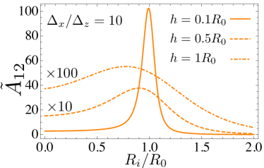
Figure 5: Plot of $\tilde{A}_{12}$ defined in Eq. (33) as function of $R_{i}/R_{0}$ for different values of $h$, assuming $R_{1}=R_{2}$ and $\Delta_{x}=10\Delta_{z}$. The value of the integral is peaked around $R_{i}\sim R_{0}$ and it increases in general by decreasing the value of $h$.

We now use Eq. (33) to determine the optimal positioning of the qubits in order to obtain shortest possible gate operation times. If we assume that the qubit splitting is predominantly along the $x$-axis ($\Delta_{x}\gg\Delta_{z}$), we obtain the behavior illustrated in Fig. 5. We conclude that for all values of $h$ the optimal positioning is below the edge of the adjacent disk. It is interesting to note that when $h\ll R_{0}$ one can obtain more than two orders of magnitude enhancement compared to the positioning previously studied in Ref. Trifunovic et al., 2013. In the opposite limit, $\Delta_{x}\ll\Delta_{z}$, we observe behavior illustrated in Fig. 6. When also $h\ll R_{0}$ we recover the same optimal positioning as before—below the edge of the disk, while when $h\sim R_{0}$, positioning the qubit anywhere below the disk yields approximately same coupling strength.

Figure 6: Plot of $\tilde{A}_{12}$ defined in Eq. (33) as function of $R_{i}/R_{0}$ for different values of $h$, assuming $R_{1}=R_{2}$ and $\Delta_{x}=0.1\Delta_{z}$. The value of the integral is peaked around $R_{i}\sim R_{0}$ only for $h\ll R_{0}$ and it increases in general by decreasing the value of $h$.

V Coupling between spin-$1/2$ and ST-qubits

In the previous sections we have considered the coupling of both spin-$1/2$ and ST qubits individually. Since each setup has its own advantages and challenges, it is interesting to show these qubits can be cross-coupled to each other and thus that hybrid spin-qubits can be formed. This opens up the possibility to take advantage of the ’best of both worlds’.

The Hamiltonian of such a hybrid system reads

$$H=H_{F}+H_{\sigma}+H_{\tau}+H_{I},$$ (34)

where the first three term on left-hand side are given by omitting the summation over $i$ in Eqns. (1),(20) and (5), respectively. The interaction term $H_{I}$ has the following form

$$H_{I} =\sum_{{\bf r}}\frac{g^{*}\mu_{0}\mu_{B}\mu}{4\pi r^{3}}\left({\bm{\sigma}}\cdot{\bf S}_{\bf r}-\frac{3({\bm{\sigma}}\cdot{\bf r})({\bf S}_{\bf r}\cdot{\bf r})}{r^{2}}\right)$$

$$+g^{*}\mu_{B}\left(\hat{B}_{\rm L}^{z}-\hat{B}_{\rm R}^{z}\right)\tau_{i}^{x},$$ (35)

with $\hat{B}_{\rm L,R}$ being given in Eq. (9) when index $i$ is omitted. Continuing along the lines of the previous sections, we perform the second order SW transformation and obtain the effective coupling between the qubits

$$H_{\rm eff} =\frac{3(\mu_{0}g^{*}\mu_{B}\,\mu)^{2}}{256\pi^{2}a^{6}}\chi_{\perp}^{\text{1D}}(\Delta)\left(\mathrm{Re}[3{A(A_{L}-A_{R})^{*}}]\tau^{x}\sigma^{z}(\Delta)\right.$$

$$+\left.(C^{*}(A_{L}-A_{R})-3B(A_{L}-A_{R})^{*})\tau^{x}\sigma^{+}(\Delta)+\text{h.c}\right)$$

$$+\{\sigma^{i}(\Delta)\rightarrow\sigma^{i},\tau^{x}\rightarrow\tau^{x}(\Delta)\},$$ (36)

where $A_{\rm L,R}$ and $A$ are calculated in Eq. (15), while $B$ and $C$ are given in Eq. (IV).

Similarly as in the previous sections, we find that the optimal coupling for the hybrid case is obtained when the spin-$1/2$ qubit is positioned below the edge of one of the two discs while one quantum well of the ST-qubit is positioned below the other disc center with the other well being below the disc edge.

VI Validity of the effective Hamiltonian

We discuss herein the validity of the effective Hamiltonian derived in Sec. III.3 and Sec. IV. In deriving those effective Hamiltonians we assumed that the state of the ferromagnet adapts practically instantaneously to the state of the two qubits at a given moment. This is true only if the dynamics of the two qubits is slow enough compared to the time scale for the ferromagnet to reach its equilibrium. To estimate the equilibration time of the ferromagnet we use the phenomenological Landau-Lifshitz-Gilbert equation Tserkovnyak et al. (2005) in standard notation

$$\partial_{t}\bm{m}=-\gamma\bm{m}\times\bm{H}_{\rm eff}+\alpha\bm{m}\times\partial_{t}\bm{m},$$ (37)

where $\bm{m}(\bm{r},t)$ is the magnetization of the (classical) ferromagnet at the given time $t$ and spatial coordinate $\bm{r}$; $\gamma=2\mu_{\rm B}/\hbar$ is the gyromagnetic ratio and $\alpha$ is Gilbert damping constant. The above equation has to be supplemented by an equation for the effective magnetic field, $\bm{H}_{\rm eff}(\bm{r},t)$.

However, here we do not aim at studying the exact dynamics of the ferromagnet but rather at giving a rough estimate of its equilibration time scale. We first estimate the time needed for the effective field, $\bm{H}_{\rm eff}(\bf r,t)$, to reach its final orientation along which the magnetization of the ferromagnet, $\bm{m}(\bf r,t)$, will eventually point. This time is roughly given by the ratio of the ferromagnet size to the relevant magnon velocity. The typical magnon energy is given by $A$, and thus the relevant magnon velocity can be estimated as $v_{M}=\sqrt{JSA}\,a/\hbar$, leading to times of $10ns$ for magnons to travel over distances of $1\mu m$ in ferromagnets. After $\bm{H}_{\rm eff}(\bf r,t)$ has reached its final value, it takes additional time for $\bm{m}(\bf r,t)$ to align along it. This time can be estimated from Eq. (37), as $T_{p}/\alpha$, where $T_{p}$ is the precession time around the effective magnetic field which can be approximated by the externally applied magnetic field (leading to the gap $\Delta_{F}$). Using the typical Gilbert damping factor of $\alpha=0.001$ Tserkovnyak et al. (2005) we arrive at the time scale of $10ps$. Therefore, the total time for the ferromagnet considered herein to reach its equilibrium is about $10ns$. This in turn leads to the bottleneck for the operation time.

Special care has to be taken for the validity of the perturbation theory employed herein, since we are working close to resonance, i.e., $\Delta-\Delta_{F}$ has to be small but still much larger than the coupling of a qubit to an individual spin of the ferromagnet. For the perturbation theory to be valid we also require the tilt of each ferromagnet spin to be sufficiently small (i.e. $\langle S_{\bf r}^{\pm}\rangle\ll 1$). The tilt of the central spin of the ferromagnetic disk can be estimated by the integral over the dogbone disk $D$

$$\langle S^{\pm}_{\bf r}\rangle=\int_{D}\chi_{\perp}({\bf r})B_{\perp}(\bf r)\,.$$ (38)

Using cylindrical coordinates we then obtain

$$\langle S_{\bf r}^{\pm}\rangle\sim\frac{\mu_{0}\mu_{B}^{2}}{2a}\int_{0}^{R}\rho d\rho\frac{1}{(\rho^{2}+h^{2})^{3/2}}\frac{S}{D\rho},$$ (39)

where $\frac{S}{D\rho}$ is the spatial decay of the transversal susceptibility and $\frac{1}{(\rho^{2}+h^{2})^{3/2}}$ is the decay of the dipolar field causing the perturbation of the ferromagnet. Even though each spin is just slightly tilted, we obtain a sizable coupling due to big number of spins involved in mediating the coupling.

VII Switching mechanisms

In this section we briefly discuss possible switching on/off mechanisms. These include changing the splitting of the qubits and moving them spatially. The former mechanism is based on the dependence of the susceptibility decay length on frequency, Trifunovic et al. (2013) see Eq. (65). It is enough to detune the qubit splitting by less then a percent to switch the qubit-qubit coupling effectively off. This is particularly feasible for the ST-qubits where qubit splitting can be controlled by all electrical means. Furthermore, the ST-qubits coupling can be switched off also by rotating them such that $A_{\rm L}=A_{\rm R}$, see Eq. (14).

The spin-$1/2$ qubits can be switched either by detuning its splitting off-resonance with the magnon gap $\Delta_{F}$ or by moving them away from the dogbone disk, see Figs. 5-6.

VIII Coupling Strengths and Operation times

In Tables 1 and 2 we present a summary of the effective coupling strengths and operation times that can be obtained in the proposed setup. We assume that the qubits are separated by a distance of $1\mu m$ and we give the remaining parameters in the table captions.

The column captions correspond to four experimentally relevant setups considered in this work (GaAs ST and spin-$1/2$ quantum dots, silicon-based quantum dots, and NV-centers). The row captions denote respectively the vertical distance $h$ between the qubit and the disk of the ferromagnet, the difference between the qubit splitting $\Delta$ and the internal splitting $\Delta_{F}$ of the ferromagnet (given in units of energy and in units of magnetic field), the obtained effective qubit-qubit interaction, and the corresponding operation time.

The operation times obtained in Tables 1 and 2 are significantly below the relaxation and decoherence times of the corresponding qubits. Indeed, for GaAs quantum dots $T_{1}=1s$ (see Ref. Amasha et al., 2008), and $T_{2}>200\mu s$ (see Ref. Bluhm et al., 2011), respectively. Here we compare to $T_{2}$ instead of $T_{2}^{*}$ since spin-echo can be performed together with two-qubit gates. Khodjasteh and Viola (2009) Alternatively, the $T_{2}^{*}$ of GaAs qubits can be increased without spin-echo by narrowing the state of the nuclear spins. Xu et al. (2009); Vink et al. (2009)

For silicon-based qubits decoherence time up to $T_{2}\approx 200\mu s$ is achievable. Pla et al. (2013) Finally decoherence times of $T_{2}^{*}\approx 20\mu s$ and $T_{2}\approx 1.8ms$ have been obtained for N-V centers in diamond. Balasubramanian et al. (2009)

In Table 3, we summarize the obtained coupling strengths and operation times obtained when a ST-qubit is cross coupled with a spin-$1/2$ qubit.

We have verified that the tilting of the ferromagnet spins given in Eq. (39) remains small. The biggest tilt we obtain (for $h=5\,nm$) is $\langle S_{\bf r}^{\pm}\rangle\approx 10^{-7}\ll 1$. Thus all the result are within the range of validity of the perturbation theory.

Table 1: The parameters used to obtain the numbers below are: Landé factor of the ferromagnet $g_{F}=2$; disk radius $R_{0}=50nm$; disk thickness $d=20nm$ ; Curie temperature $T=550K$ and thus exchange coupling $J/k_{B}\approx 824K$; lattice constant of the ferromagent $a=4\textup{\AA}$. We consider the case $\Delta_{x}\ll\Delta_{z}$.

	GaAs ST QD	GaAs ST QD	GaAs spin-$1/2$ QD	Silicon-based QD	NV-center
$\Delta_{x}\ll\Delta_{z}$	$|g^{*}|=0.4$	$|g^{*}|=0.4$	$|g^{*}|=0.4$	$|g^{*}|=2$	$|g^{*}|=2$
Distance $h$	$50\,nm$	$50\,nm$	$50\,nm$	$25\,nm$	$5\,nm$
Splitting $\Delta_{F}-\Delta$	$1\,\mu eV$ ($43.2\,mT$)	$0.5\mu eV$ ($21.6mT$)	$10^{-2}\,\mu eV$ ($0.4\,mT$)	$10^{-2}\,\mu eV$ ($0.1\,mT$)	$10^{-1}\,\mu eV$ ($0.9\,mT$)
Coupling strength (CS)	$1.4\times 10^{-9}\,eV$	$1.4\times 10^{-8}$	$2\times 10^{-10}\,eV$	$2.4\times 10^{-8}\,eV$	$1.8\times 10^{-8}\,eV$
Operation time (OS)	$470\,ns$	$47ns$	$3.3\,\mu s$	$27.4\,ns$	$36.6\,ns$

Table 2: We use the same parameters as in Table 1 but consider the case $\Delta_{x}\gg\Delta_{z}$.

	GaAs spin-$1/2$ QD	Silicon-based QD	NV-center
$\Delta_{x}\gg\Delta_{z}$	$|g^{*}|=0.4$	$|g^{*}|=2$	$|g^{*}|=2$
Distance $h$	$50\,nm$	$25\,nm$	$5\,nm$
Splitting $\Delta_{F}-\Delta$	$10^{-2}\,\mu eV$ ($0.4\,mT$)	$10^{-2}\,\mu eV$ ($0.1\,mT$)	$10^{-1}\,\mu eV$ ($0.9\,mT$)
Coupling strength	$1.2\times 10^{-10}\,eV$	$1.8\times 10^{-8}\,eV$	$3.6\times 10^{-8}\,eV$
Operation time	$5.5\,\mu s$	$36.6\,ns$	$18.3\,ns$

Table 3: We use the same parameters as in Table 1 and choose the splitting $\Delta_{F}-\Delta=10^{-2}\,\mu eV$ for the ST-qubit (the splitting of the other qubit is taken from Table 1) to determine the coupling strengths and operation times achieved in the hybrid case. The column caption of the table labels GaAs ST-QD, while the row captions label the three other qubit systems, considered in this work, to which it can be hybridized. The left panel corresponds to the case $\Delta_{x}\ll\Delta_{z}$ while the right panel corresponds to $\Delta_{x}\gg\Delta_{z}$.

$\Delta_{x}\ll\Delta_{z}$	GaAs ST QD
	Coupling strength	Operation time
GaAs spin-$1/2$ QD	$1.7\times 10^{-9}\,eV$	$387\,ns$
Silicon-based QD	$1.8\times 10^{-8}\,eV$	$36.6\,ns$
NV-center	$1.6\times 10^{-8}\,eV$	$41.1\,ns$

$\Delta_{x}\gg\Delta_{z}$	GaAs ST QD
	Coupling strength	Operation time
GaAs spin-$1/2$ QD	$1.3\times 10^{-9}\,eV$	$506\,ns$
Silicon-based QD	$1.6\times 10^{-8}\,eV$	$41.1\,ns$
NV-center	$2.2\times 10^{-8}\,eV$	$29.9\,ns\,ns$

IX Conclusions

We have proposed and studied a model that allows coherent coupling of distant spin qubits. The idea is to introduce a piece of ferromagnetic material between qubits to which they couple dipolarly. A dogbone shape of the ferromagnet is the best compromise since it allows both strong coupling of the qubits to the ferromagnet and long-distance coupling because of its slowly decaying 1D spin-spin susceptibility. We have derived an effective Hamiltonian for the qubits in the most general case where the qubits are positioned arbitrarily with respect to the dogbone. We have calculated the optimal position for the effective qubit-qubit coupling to be strongest and estimated it. For both the singlet-triplet (ST) and spin-$1/2$ qubits, interaction strengths of $10^{-2}{\rm\mu eV}$ can be achieved. Since decoherence effects induced by the coupling to the ferromagnet are negligible, Trifunovic et al. (2013) we obtain error thresholds of about $10^{-4}$ for ST-qubits and for spin-$1/2$ qubits. In both cases this is good enough to implement the surface code error correction. Raussendorf and Harrington (2007) Finally, for both types of qubits we have explicitly constructed the sequence to implement a CNOT gate achievable with a fidelity of more than 99.9%

Our analysis is general and is not restricted to any special types of qubits as long as they couple dipolarly to the ferromagnet. Furthermore, the only relevant quantity of the coupler is its spin-spin susceptibility. Hence, our analysis is valid for any kind of coupler (and not just a ferromagnet) that has a sufficiently slowly decaying susceptibility.

This quantum computing architecture retains all the single qubit gates and measurement aspects of earlier approaches, but allows qubit spacing at distances of order 1 $\mu m$ for two- qubit gates, achievable with the state-of-the-art semiconductor technology.

X Acknowledgment

We would like to thank A. Yacoby, A. Morello, and C. Kloeffel for useful discussions. This work was supported by the Swiss NSF, NCCR QSIT, and IARPA.

Appendix A Holstein-Primakoff transformation

For the sake of completeness we derive in this Appendix explicit expressions for the different spin-spin correlators used in this work

$$C^{\alpha\beta}(\omega,{\bf q})=\langle S_{{\bf q}}^{\alpha}(\omega)S_{-{\bf q}}^{\beta}(0)\rangle\,.$$ (40)

For this purpose, we make use of a Holstein-Primakoff transformation

$$S_{i}^{z} = -S+n_{i},\,\,\,S_{i}^{-}=\sqrt{2S}\sqrt{1-\frac{n_{i}}{2S}}a_{i},\,\,\,\mathrm{and}$$

$$S_{i}^{+} = \left(S_{i}^{-}\right)^{\dagger},$$ (41)

in the limit $n_{i}\ll 2S$, with $a_{i}$ satisfying bosonic commutation relations and $n_{i}=a_{i}^{\dagger}a_{i}$ Nolting and Ramakanth (2009). The creation operators $a_{i}^{\dagger}$ and annihilation operators $a_{i}$ satisfy bosonic commutation relations and the associated particles are called magnons. The corresponding Fourier transforms are straightforwardly defined as $a_{{\bf q}}^{\dagger}=\frac{1}{\sqrt{N}}\sum_{i}e^{-i{\bf q}\cdot{\bf R}_{i}}a_{i}$. In harmonic approximation, the Heisenberg Hamiltonian $H_{F}$ reads

$$H_{F}\approx\sum_{\bf q}\epsilon_{{\bf q}}a_{{\bf q}}^{\dagger}a_{{\bf q}}\,,$$ (42)

where $\epsilon_{\bf q}=\omega_{\bf q}+\Delta_{F}=4JS[3-(\cos(q_{x})+\cos(q_{y})+\cos(q_{z}))]+\Delta_{F}$ is the spectrum for a cubic lattice with lattice constant $a=1$ and the gap $\Delta_{F}$ is induced by the external magnetic field or anisotropy of the ferromagnet.

Appendix B Transverse correlators $\langle S_{{\bf q}}^{+}(t)S_{-{\bf q}}^{-}(0)\rangle$

Let us now define the Fourier transforms in the harmonic approximation

$$S_{{\bf q}}^{+} = \frac{1}{\sqrt{N}}\sum_{i}e^{-i{\bf q}\cdot{\bf r}_{i}}S_{i}^{+}\approx\frac{\sqrt{2S}}{\sqrt{N}}\sum_{i}e^{-i{\bf q}\cdot{\bf r}_{i}}a_{i}^{\dagger}=\sqrt{2S}a_{-{\bf q}}^{\dagger}\,,$$

$$S_{-{\bf q}}^{-} = \frac{1}{\sqrt{N}}\sum_{i}e^{i{\bf q}\cdot{\bf r}_{i}}S_{i}^{-}\approx\frac{\sqrt{2S}}{\sqrt{N}}\sum_{i}e^{i{\bf q}\cdot{\bf r}_{i}}a_{i}=\sqrt{2S}a_{-{\bf q}}\,.$$ (43)

From this it directly follows that

$$C^{+-}(t,{\bf q}) =\langle S_{{\bf q}}^{+}(t)S_{-{\bf q}}^{-}(0)\rangle$$

$$=2S\langle a_{-{\bf q}}^{\dagger}(t)a_{-{\bf q}}\rangle=2Se^{i\epsilon_{\bf q}t}n_{{\bf q}}\,,$$ (44)

with $\epsilon_{\bf q}\approx D{\bf q}^{2}+\Delta_{F}$ in the long-wavelength approximation.

The Fourier transform is then given by

$$C^{+-}(\omega,{\bf q}) = \frac{1}{\sqrt{2\pi}}\int_{-\infty}^{\infty}dte^{-i\omega t}C^{+-}(t,{\bf q})$$ (45)

$$= \underbrace{\frac{1}{\sqrt{2\pi}}\int_{-\infty}^{\infty}dte^{i(\epsilon_{\bf q}-\omega)t}}_{\sqrt{2\pi}\delta(\epsilon_{\bf q}-\omega)}2Sn_{\bf q}$$

$$= \sqrt{2\pi}2S\delta(\epsilon_{\bf q}-\omega)\frac{1}{e^{\beta\omega}-1}\,.$$

The corresponding correlator in real space becomes ($q=|{\bf q}|$)

$$C^{+-}(\omega,{\bf r}) = \frac{1}{(2\pi)^{3/2}}\int d{\bf q}e^{i{\bf q}\cdot{\bf r}}C^{+-}(\omega,{\bf q})$$

$$= \frac{\sqrt{2\pi}}{(2\pi)^{3/2}}2S\frac{1}{e^{\beta\omega}-1}\int d{\bf q}\delta(D{\bf q}^{2}+\Delta_{F}-\omega)e^{i{\bf q}\cdot{\bf r}}$$

$$= \frac{2S}{e^{\beta\omega}-1}\int_{-1}^{1}\int_{0}^{\infty}dqdxq^{2}\delta(Dq^{2}+\Delta_{F}-\omega)e^{iqrx}$$

$$= \frac{4S}{r}\frac{1}{e^{\beta\omega}-1}\int_{0}^{\infty}dqq\delta(Dq^{2}+\Delta_{F}-\omega)\sin(qr)\,.$$

Let us now perform the following substitution

$$y=Dq^{2},$$ (47)

which gives for $\omega>\Delta_{F}$

$$C^{+-}(\omega,{\bf r}) =\frac{4S/r}{2D(e^{\beta\omega}-1)}\int_{0}^{\infty}dy\delta(y+\Delta_{F}-\omega)\times$$

$$\times\sin\left(\sqrt{\frac{y}{D}}r\right)$$ (48)

$$=\frac{2S}{D}\frac{1}{e^{\beta\omega}-1}\frac{\sin(\sqrt{(\omega-\Delta_{F})/D}r)}{r}\,.$$

We remark that

$$C^{+-}(\omega,{\bf r})=0,\quad\omega<\Delta_{F}.$$ (49)

We note the diverging behavior of the above correlation function for $\Delta_{F}=0$ and $\omega\rightarrow 0$, namely

$$\lim\limits_{\omega\rightarrow 0}\frac{1}{e^{\beta\omega}-1}\frac{\sin\left(\sqrt{\frac{\omega}{D}r}\right)}{r} = \lim\limits_{\omega\rightarrow 0}\frac{\sqrt{\omega/D}r}{r\beta\omega}$$ (50)

$$\rightarrow\frac{1}{\sqrt{D}\beta}\frac{1}{\sqrt{\omega}}\,.$$

Similarly, it is now easy to calculate the corresponding commutators and anticommutators. Let us define

$$S_{\perp}(t,{\bf q}):=\frac{1}{2}\{S_{{\bf q}}^{+}(t),S_{-{\bf q}}^{-}(0)\}\,.$$ (51)

It is then straightforward to show that

$$S_{\perp}(t,{\bf q}) = Se^{i\epsilon_{\bf q}t}(1+2n_{{\bf q}})\,,$$ (52)

and therefore

$$S_{\perp}(\omega,{\bf q}) = \frac{S}{\sqrt{2\pi}}\int_{-\infty}^{\infty}e^{i(\epsilon_{\bf q}-\omega)t}(1+2n_{\bf q})$$ (53)

$$= S\sqrt{2\pi}\delta(\epsilon_{\bf q}-\omega)\left(1+2\frac{1}{e^{\beta\omega}-1}\right).$$

Following essentially the same steps as the ones performed above, we obtain the 3D real space anticommutator for $\omega>\Delta_{F}$

$$S^{\mathrm{3D}}_{\perp}(\omega,{\bf q}) = S\coth(\beta\omega/2)\times$$

$$\times\int_{-1}^{1}\int_{0}^{\infty}dxdqq^{2}e^{iqrx}\delta(\epsilon_{{\bf q}}-\omega)$$

$$= \frac{S}{D}\coth(\beta\omega/2)\frac{\sin(\sqrt{(\omega-\Delta_{F})/D}r)}{r}\,.$$

Let us now finally calculate the transverse susceptibility defined as

$$\chi_{\perp}(t,{\bf q}) = -i\theta(t)[S_{{\bf q}}^{+}(t),S_{-{\bf q}}^{-}(0)]\,.$$ (56)

As before, in the harmonic approximation, one finds

$$\chi_{\perp}(t,{\bf q}) = i\theta(t)2Se^{i\epsilon_{\bf q}t}\,.$$ (57)

In the frequency domain, we then have

$$\chi_{\perp}(\omega,{\bf q}) =\frac{2iS}{\sqrt{2\pi}}\int_{0}^{\infty}dte^{i(\epsilon_{\bf q}-\omega)t-\eta t}$$ (58)

$$=-\frac{2S}{\sqrt{2\pi}}\frac{1}{\epsilon_{\bf q}-\omega+i\eta}\,,$$

and thus in the small ${\bf q}$ expansion

$$\chi_{\perp}(\omega,{\bf q}) = -\frac{2S}{\sqrt{2\pi}}\frac{1}{D{\bf q}^{2}+\Delta_{F}-\omega+i\eta}\,.$$ (59)

In real space, for the three-dimensional case, we obtain

$$\chi^{\text{3D}}_{\perp}(\omega,{\bf r}) = -\frac{2S}{\sqrt{2\pi}}\frac{2\pi}{(2\pi)^{3/2}}\int_{0}^{\infty}\int_{-1}^{1}dxdqq^{2}\frac{1}{D{\bf q}^{2}+\Delta_{F}-\omega+i\eta}e^{iqrx}$$ (60)

$$= -\frac{4S}{\sqrt{2\pi}}\frac{2\pi}{(2\pi)^{3/2}}\frac{1}{r}\int_{0}^{\infty}dqq\frac{1}{Dq^{2}+\Delta_{F}-\omega+i\eta}\sin(qr)\,.$$

Making use of the Plemelj formula we obtain for $\omega>\Delta_{F}$

$$\chi^{\text{3D}}_{\perp}(\omega,{\bf r}) = -\frac{2S}{\sqrt{2\pi}}\frac{2\pi}{(2\pi)^{3/2}}\frac{1}{r}\int_{-\infty}^{\infty}dqq\frac{1}{Dq^{2}+\Delta_{F}-\omega+i\eta}\sin(qr)$$ (61)

$$= -\frac{2S}{\sqrt{2\pi}}\frac{2\pi}{(2\pi)^{3/2}}\frac{1}{r}P\int_{-\infty}^{\infty}dq\frac{q}{Dq^{2}+\Delta_{F}-\omega}\sin(qr)+i\frac{2S}{\sqrt{2\pi}}\frac{2\pi^{2}}{(2\pi)^{3/2}}\frac{1}{r}\int_{-\infty}^{\infty}dqq\delta(Dq^{2}+\Delta_{F}-\omega)\sin(qr)$$

$$= -\frac{S}{D}\frac{\cos(r\sqrt{(\omega-\Delta_{F})/D})}{r}+i\frac{S}{2D}\frac{\sin(\sqrt{(\omega-\Delta_{F})/D}r)}{r}\,.$$

It is worth pointing out that the imaginary part of the susceptibility vanishes

$$\chi^{\text{3D}}_{\perp}(\omega,{\bf r})^{\prime\prime}=0,\quad\omega<\Delta_{F},$$ (62)

and therefore the susceptibility is purely real and takes the form of a Yukawa potential

$$\chi_{\perp}^{\text{3D}}(\omega,{\bf r})=-\frac{S}{D}\frac{e^{-r/l_{F}}}{r},\quad\omega<\Delta_{F},$$ (63)

where $l_{F}=\sqrt{\frac{D}{\Delta_{F}-\omega}}$.

Note also that the imaginary part of the transverse susceptibility satisfies the well-know fluctuation dissipation theorem

$$S^{\mathrm{3D}}_{\perp}(\omega,{\bf r}) = \coth(\beta\omega/2)\chi^{\text{3D}}_{\perp}(\omega,{\bf r})^{\prime\prime}\,.$$ (64)

In three dimensions the susceptibility decays as $1/r$, where $r$ is measured in lattice constants. For distances of order of $1\mu m$ this leads to a reduction by four orders of magnitude.

For quasi one-dimensional ferromagnets such a reduction is absent and the transverse susceptibility reads

$$\chi_{\perp}^{\text{1D}}(\omega,r)=-\frac{S}{D}l_{F}e^{-r/l_{F}},\quad\omega<\Delta_{F},$$ (65)

where $l_{F}$ is defined as above and the imaginary part vanishes as above, i.e.,

$$\chi_{\perp}^{\text{1D}}(\omega,r)^{\prime\prime}=0,\quad\omega<\Delta_{F}.$$ (66)

Similarly for $\omega>\Delta_{F}$ we have

$$\chi_{\perp}^{\text{1D}}(\omega,r)=S\frac{\sin\left(\sqrt{(\omega-\Delta_{F})/D}r\right)}{\sqrt{D(\omega-\Delta_{F})}}\,,$$ (67)

and

$$\chi_{\perp}^{\text{1D}}(\omega,r)^{\prime\prime}=\frac{S}{2D}\sqrt{\frac{D}{\omega-\Delta_{F}}}\cos\left(\sqrt{(\omega-\Delta_{F})/D}r\right)\,.$$ (68)

Appendix C Longitudinal correlators $\langle S_{{\bf q}}^{z}(t)S_{-{\bf q}}^{z}(0)\rangle$

The longitudinal susceptibility reads

$$\chi_{\parallel}(t,{\bf q}) = -i\theta(t)[S_{{\bf q}}^{z}(t),S_{-{\bf q}}^{z}(0)]$$

$$= -\theta(t)\frac{1}{N}\sum_{{\bf q}^{\prime},{\bf q}^{\prime\prime}}e^{it(\epsilon_{{\bf q}^{\prime}}-\epsilon_{{\bf q}^{\prime}+{\bf q}})}\langle[a_{{\bf q}^{\prime}}^{\dagger}a_{{\bf q}^{\prime}+{\bf q}},a_{{\bf q}^{\prime\prime}}^{\dagger}a_{{\bf q}^{\prime\prime}-{\bf q}}]\rangle\,.$$

Applying Wick’s theorem and performing a Fourier transform, we obtain the susceptibility in frequency domain

$$\chi_{\parallel}(\omega,{\bf q})=-\frac{1}{N}\sum_{{\bf k}}\frac{n_{\bf k}-n_{{\bf k}+{\bf q}}}{\omega-\epsilon_{{\bf k}+{\bf q}}+\epsilon_{\bf k}+i\eta}\,,$$ (70)

where $n_{\bf k}$ is the magnons occupation number, which is given by the Bose-Einstein distribution

$$n_{k}=\frac{1}{e^{\beta\epsilon_{\bf k}}-1}\,,$$ (71)

where $\epsilon_{\bf k}$ is again the magnon spectrum ($\epsilon_{\bf k}=\omega_{\bf k}+\Delta_{F}\approx D{\bf k}^{2}+\Delta_{F}$ for small $k$). Note that the transverse susceptibility dominates, since its ratio to longitudinal one is proportional to $1/S\ll 1$. Furthermore, the longitudinal susceptibility is $\propto n_{k}\ll 1$ and thus vanishes at zero temperature, while this is not the case for the transverse.

Since we are interested in the decoherence processes caused by the longitudinal fluctuations, we calculate the imaginary part of $\chi_{\parallel}(\omega,{\bf q})$ which is related to the fluctuations via the fluctuation-dissipation theorem. Performing a small ${\bf q}$ expansion and assuming without loss of generality $\omega>0$, we obtain

$$\chi^{\text{3D}}_{\parallel}(\omega,{\bf q})^{\prime\prime} = \frac{\pi}{(2\pi)^{3}}\int d{\bf k}(n_{\bf k}-n_{{\bf k}+{\bf q}})\delta(\omega_{\bf k}-\omega_{{\bf k}+{\bf q}}+\omega)$$ (72)

$$= \frac{1}{4\pi}\int_{0}^{\infty}dkk^{2}\int_{-1}^{1}dx\left(\frac{1}{e^{\beta(\Delta_{F}+Dk^{2})}-1}-\frac{1}{e^{\beta(\omega+\Delta_{F}+Dk^{2})}-1}\right)\delta(\omega-Dq^{2}-2Dkqx)$$

$$= \frac{1}{4\pi}\int_{0}^{\infty}dkk^{2}\int_{-1}^{1}dx\left(\frac{1}{e^{\beta(\Delta_{F}+Dk^{2})}-1}-\frac{1}{e^{\beta(\omega+\Delta_{F}+Dk^{2})}-1}\right)\delta\left(k-\frac{\omega-Dq^{2}}{2Dqx}\right)\left|\frac{1}{2Dqx}\right|$$

$$= \frac{1}{4\pi}\int_{-1}^{1}dx\left|\frac{1}{2Dqx}\right|\left(\frac{\omega-Dq^{2}}{2Dqx}\right)^{2}\left(\frac{1}{e^{\beta\left(\Delta_{F}+D\left(\frac{\omega-Dq^{2}}{2Dqx}\right)^{2}\right)}-1}-\frac{1}{e^{\beta\left(\omega+\Delta_{F}+D\left(\frac{\omega-Dq^{2}}{2Dqx}\right)^{2}\right)}-1}\right)\theta\left(\frac{\omega-Dq^{2}}{2Dqx}\right)$$

$$= \frac{1}{4\pi}\int_{0}^{1}dx\frac{1}{2Dqx}\left(\frac{\omega-Dq^{2}}{2Dqx}\right)^{2}\left(\frac{1}{e^{\beta\left(\Delta_{F}+D\left(\frac{\omega-Dq^{2}}{2Dqx}\right)^{2}\right)}-1}-\frac{1}{e^{\beta\left(\omega+\Delta_{F}+D\left(\frac{\omega-Dq^{2}}{2Dqx}\right)^{2}\right)}-1}\right).$$

Next, since we are interested in the regime where $\omega\gg T$ (and thus $\beta\omega\gg 1$), we have $n_{\bm{k}}\gg n_{\bm{k+q}}$. Furthermore, we approximate the distribution function $n_{\bm{k}}=\frac{e^{-\beta(\Delta_{F}+\omega_{\bm{k}})}}{1-e^{-\beta\Delta_{F}}+\beta\omega_{\bm{k}}}$ (this is valid when $\beta\omega_{\bf k}\ll 1$) and arrive at the following expression

$$\chi^{\text{3D}}_{\parallel}(\omega,{\bf q})^{\prime\prime} =\frac{1}{4\pi}\int_{0}^{1}dx\frac{1}{2Dqx}\left(\frac{\omega-Dq^{2}}{2Dqx}\right)^{2}\frac{e^{-\beta\left(\Delta_{F}+D\left(\frac{\omega-Dq^{2}}{2Dqx}\right)^{2}\right)}}{1-e^{-\beta\Delta_{F}}+\beta D\left(\frac{\omega-Dq^{2}}{2Dqx}\right)^{2}}$$

$$=-\frac{e^{1-e^{-\beta\Delta_{F}}-\beta\Delta_{F}}}{4\beta D^{2}q}\mathrm{Ei}\left(e^{-\beta\Delta_{F}}+\frac{1}{4}\left(-4-\beta Dq^{2}+2\beta\omega-\frac{\beta\omega^{2}}{Dq^{2}}\right)\right)\,,$$ (73)

where $\mathrm{Ei}(z)$ is the exponential integral function. We also need the the real space represenation obtained after inverse Fourier transformation,

$$\chi^{\text{3D}}_{\parallel}(\omega,{\bf r})^{\prime\prime} =\sqrt{\frac{2}{\pi}}\frac{1}{r}\int_{0}^{\infty}dqq\chi^{\text{3D}}_{\parallel}(\omega,q)^{\prime\prime}\sin(qr)\,.$$ (74)

In order to perform the above integral we note that the imaginary part of the longitudinal susceptibility, given by Eq. (C), is peaked around $q=\sqrt{\omega/D}$ with the width of the peak ($1/\sqrt{\beta D}$) much smaller than its position in the regime we are working in ($\omega\gg T$). For $\bf r=0$, the integration over $q$ can be then performed approximately and yields the following expression

$$\chi^{\text{3D}}_{\parallel}(\omega,{\bf r=0})^{\prime\prime} =\frac{\sqrt{\pi}e^{-e^{-\beta\Delta_{F}}-3\beta\Delta_{F}/2}}{2\beta^{2}D^{3}}\left(e^{e^{-\beta\Delta_{F}}+\beta\Delta_{F}/2}\right.$$

$$-e\sqrt{\pi}\sqrt{e^{\beta\Delta_{F}}-1}$$ (75)

$$\times\left.\mathrm{Erfc}(e^{-\beta\Delta_{F}/2}\sqrt{e^{\beta\Delta_{F}}-1})\right)\sqrt{\beta\omega}\,,$$

where $\mathrm{Erfc}(z)$ denotes the complementary error function. It is readily observed from the above expression that the longitudinal fluctuations are exponentially suppressed by the gap. Assuming that $\Delta_{F}\gg T$, we obtain the following simplified expression

$$\chi^{\text{3D}}_{\parallel}(\omega,{\bf r=0})^{\prime\prime} =\frac{\sqrt{\pi}-e\pi\mathrm{Erfc}(1)}{2\beta^{2}D^{3}}e^{-\beta\Delta_{F}}\sqrt{\beta\omega}\,.$$ (76)

We observe that, since $J(\omega)=\chi_{\parallel}(\omega,{\bf r})^{\prime\prime}$, the longitudinal noise of the ferromagnet is—as the transverse one—sub-ohmic DiVincenzo and Loss (2005).

Next we calculate the longitudinal fluctuations for the case of a quasi- one-dimensional ferromagnet ($\Delta_{F}\gg T$) and obtain

$$\chi_{\parallel}^{\text{1D}}(\omega,r=0)^{\prime\prime} =\frac{1}{4\pi}\int_{-\infty}^{\infty}dk\int_{-\infty}^{\infty}dq\left(\frac{1}{e^{\beta(\Delta_{F}+Dk^{2})}-1}\right.$$

$$-\left.\frac{1}{e^{\beta(\omega+\Delta_{F}+Dk^{2})}-1}\right)\delta(\omega-Dq^{2}-2Dkq)$$

$$=\int_{-\infty}^{\infty}dk\frac{e^{-\beta Dk^{2}}}{1-e^{-\beta\Delta_{F}}+\beta Dk^{2}}\frac{1}{D\sqrt{k^{2}+\omega/D}}$$

$$=\frac{\gamma}{D\sqrt{\beta\omega}}e^{-\beta\Delta_{F}}\,,$$ (77)

where $\gamma$ is a numerical factor of order 1.

Appendix D Rotated Hamiltonian for CNOT Hate

Here we give the general for of the matrix $\hat{\widetilde{H}}$ entering Eq. (31).

$$\tilde{\mathcal{H}}_{12} =\frac{3\left(\Delta_{z}\Delta_{z}^{-}(C_{2}^{\prime\prime}(-6\Delta_{x}A_{1}^{\prime}+B_{1}\Delta_{z}^{-}+3C_{1}^{\prime}\Delta_{z}^{+})+2\Delta_{x}A_{1}^{\prime\prime}(B_{2}+3C_{2}^{\prime})+C_{1}^{\prime\prime}(B_{2}\Delta_{z}^{-}-3C_{2}^{\prime}\Delta_{z}^{+}))\right)}{32\Delta^{3}}$$ (78)

$$+\frac{3\Delta_{x}i\left(12A_{2}\Delta\Delta_{x}A_{1}^{*}-12A_{1}\Delta\Delta_{x}A_{2}^{*}+\Delta_{x}\left(-4\Delta_{x}A_{1}^{\prime}(B_{2}+3C_{2})+4A_{1}B_{2}\Delta_{x}+\Delta_{z}^{-}\left(3C_{1}C_{2}^{*}+2i(B_{1}C_{2}^{\prime\prime}+B_{2}C_{1}^{\prime\prime})\right)\right)\right)}{64\Delta^{3}}$$

$$+\frac{3\Delta_{x}i\left(12A_{1}\Delta_{x}^{2}C_{2}^{\prime}+3C_{1}^{*}\Delta_{z}^{-}(2A_{2}\Delta-C_{2}\Delta_{x})+\left(2B_{1}\Delta A_{2}^{\prime\prime}\Delta_{z}^{-}+3iC_{1}\Delta A_{2}^{*}\Delta_{z}^{-}\right)\right)}{64\Delta^{3}}\,,$$

$$\tilde{\mathcal{H}}_{13} =\frac{2\left(\Delta_{z}^{z}(B_{2}\Delta_{x}(B_{1}-3C_{1}^{\prime})-3B_{1}(2\Delta_{z}A_{2}^{\prime}+\Delta_{x}C_{2}^{\prime}))-6B_{2}\Delta_{x}^{2}A_{1}^{\prime}\right)+18\Delta_{z}A_{2}^{*}(2A_{1}\Delta_{x}+C_{1}\Delta-C_{1}\Delta_{z})}{{64\Delta^{2}}}$$ (79)

$$+\frac{9\Delta_{x}C_{2}^{*}(2A_{1}\Delta_{x}+C_{1}\Delta-C_{1}\Delta_{z})+9C_{1}^{*}\Delta_{z}^{-}(2A_{2}\Delta_{z}+C_{2}\Delta_{x})+18\Delta_{x}A_{1}^{*}(2A_{2}\Delta_{z}+C_{2}\Delta_{x})}{64\Delta^{2}},$$

$$\tilde{\mathcal{H}}_{23} =\frac{3i\left(2i(\Delta_{x}(\Delta_{z}^{-}(B_{1}C_{2}^{\prime\prime}+B_{2}C_{1}^{\prime\prime})+2iB_{2}\Delta_{x}A_{1}^{\prime})+2iB_{1}\Delta_{z}A_{2}^{\prime}\Delta_{z}^{-})+4\left(A_{1}B_{2}\Delta_{x}^{2}+A_{2}B_{1}\Delta_{z}\Delta_{z}^{-}\right)\right)}{64\Delta^{2}}$$ (80)

$$+\frac{3i\left(6\Delta_{z}A_{2}^{*}(-2A_{1}\Delta_{x}-C_{1}\Delta+C_{1}\Delta_{z})-6\Delta_{x}A_{1}^{*}(C_{2}\Delta_{x}-2A_{2}\Delta_{z})+3\Delta_{x}C_{2}^{*}(2A_{1}\Delta_{x}-C_{1}\Delta+C_{1}\Delta_{z})\right)}{64\Delta^{2}}$$

$$+\frac{3i\left(3C_{1}^{*}\Delta_{z}^{-}(2A_{2}\Delta_{z}+C_{2}\Delta_{x})\right)}{64\Delta^{2}},$$

$$\tilde{\mathcal{H}}_{11} =\frac{2(6B_{2}\Delta_{x}\Delta_{z}A_{1}^{\prime}-\Delta_{z}^{-}(6B_{1}\Delta_{x}A_{2}^{\prime}+B_{2}\Delta_{z}(B_{1}-3C_{1}^{\prime})-3B_{1}\Delta_{z}C_{2}^{\prime}))+18\Delta_{x}A_{2}^{*}(2A_{1}\Delta_{x}+C_{1}\Delta-C_{1}\Delta_{z})}{32\Delta^{2}}$$

$$+\frac{18\Delta_{x}A_{1}^{*}(2A_{2}\Delta_{x}-C_{2}\Delta_{z})+9\Delta_{z}C_{2}^{*}(-2A_{1}\Delta_{x}-C_{1}\Delta+C_{1}\Delta_{z})-9C_{1}^{*}\Delta_{z}^{-}(C_{2}\Delta_{z}-2A_{2}\Delta_{x})}{32\Delta^{2}},$$ (81)

$$\tilde{\mathcal{H}}_{22} =\frac{2(6B_{2}\Delta_{x}A_{1}^{\prime}+\Delta_{z}^{-}(B_{1}(B_{2}+3C_{2}^{\prime})+3B_{2}C_{1}^{\prime}))-9C_{2}^{*}(2A_{1}\Delta_{x}-C_{1}\Delta+C_{1}\Delta_{z})-18C_{2}\Delta_{x}A_{1}^{*}+9C_{2}C_{1}^{*}\Delta_{z}^{-}}{32\Delta},$$ (82)

$$\tilde{\mathcal{H}}_{33} =0,$$ (83)

and the rest of the components $\tilde{\mathcal{H}}_{ij}$ are obtain from $\tilde{\mathcal{H}}_{ji}$ by exchanging $i\leftrightarrow j$.

References

- Kloeffel and Loss (2013) C. Kloeffel and D. Loss, Annual Review of Condensed Matter Physics 4, 51 (2013).
- Levy (2002) J. Levy, Phys. Rev. Lett. 89, 147902 (2002).
- Amasha et al. (2008) S. Amasha, K. MacLean, I. P. Radu, D. M. Zumbühl, M. A. Kastner, M. P. Hanson, and A. C. Gossard, Phys. Rev. Lett. 100, 046803 (2008).
- Bluhm et al. (2011) H. Bluhm, S. Foletti, I. Neder, M. Rudner, D. Mahalu, V. Umansky, and A. Yacoby, Nat. Phys. 7, 109 (2011).
- Petta et al. (2005) J. R. Petta, A. C. Johnson, J. M. Taylor, E. A. Laird, A. Yacoby, M. D. Lukin, C. M. Marcus, M. P. Hanson, and A. C. Gossard, Science 309, 2180 (2005).
- Koppens et al. (2008) F. H. L. Koppens, K. C. Nowack, and L. M. K. Vandersypen, Phys. Rev. Lett. 100, 236802 (2008).
- Brunner et al. (2011) R. Brunner, Y.-S. Shin, T. Obata, M. Pioro-Ladrière, T. Kubo, K. Yoshida, T. Taniyama, Y. Tokura, and S. Tarucha, Phys. Rev. Lett. 107, 146801 (2011).
- Shulman et al. (2012) M. D. Shulman, O. E. Dial, S. P. Harvey, H. Bluhm, V. Umansky, and A. Yacoby, Science 336, 202 (2012).
- Pla et al. (2013) J. J. Pla, K. Y. Tan, J. P. Dehollain, W. H. Lim, J. J. L. Morton, F. A. Zwanenburg, D. N. Jamieson, A. S. Dzurak, and A. Morello, ArXiv e-prints (2013), arXiv:1302.0047 .
- Pla et al. (2012) J. J. Pla, K. Y. Tan, J. P. Dehollain, W. H. Lim, J. J. L. Morton, D. N. Jamieson, A. S. Dzurak, and A. Morello, Nature 489, 541 (2012).
- Dobrovitski et al. (2013) V. Dobrovitski, G. Fuchs, A. Falk, C. Santori, and D. Awschalom, Ann. Rev. Condens. Matter Phys. 4, 23 (2013).
- Choi et al. (2000) M.-S. Choi, C. Bruder, and D. Loss, Phys. Rev. B 62, 13569 (2000).
- Leijnse and Flensberg (2013) M. Leijnse and K. Flensberg, ArXiv e-prints (2013), arXiv:1303.3507 .
- Trif et al. (2008) M. Trif, F. Troiani, D. Stepanenko, and D. Loss, Phys. Rev. Lett. 101, 217201 (2008).
- Wallraff et al. (2004) A. Wallraff, D. I. Schuster, A. Blais, L. Frunzio, R.-S. Huang, J. Majer, S. Kumar, S. M. Girvin, and R. J. Schoelkopf, Nature 431, 162 (2004).
- Rikitake and Imamura (2005) Y. Rikitake and H. Imamura, Phys. Rev. B 72, 033308 (2005).
- Flensberg and Marcus (2010) K. Flensberg and C. M. Marcus, Phys. Rev. B 81, 195418 (2010).
- Trifunovic et al. (2012) L. Trifunovic, O. Dial, M. Trif, J. R. Wootton, R. Abebe, A. Yacoby, and D. Loss, Phys. Rev. X 2, 011006 (2012).
- Flindt et al. (2006) C. Flindt, A. S. Sørensen, and K. Flensberg, Phys. Rev. Lett. 97, 240501 (2006).
- Trif et al. (2007) M. Trif, V. N. Golovach, and D. Loss, Phys. Rev. B 75, 085307 (2007).
- Trifunovic et al. (2013) L. Trifunovic, F. L. Pedrocchi, and D. Loss, ArXiv e-prints (2013), arXiv:1302.4017 .
- Klinovaja et al. (2012) J. Klinovaja, D. Stepanenko, B. I. Halperin, and D. Loss, Phys. Rev. B 86, 085423 (2012).
- Stepanenko et al. (2012) D. Stepanenko, M. Rudner, B. I. Halperin, and D. Loss, Phys. Rev. B 85, 075416 (2012).
- Imamoglu et al. (1999) A. Imamoglu, D. D. Awschalom, G. Burkard, D. P. DiVincenzo, D. Loss, M. Sherwin, and A. Small, Phys. Rev. Lett. 83, 4204 (1999).
- Tanamoto et al. (2008) T. Tanamoto, K. Maruyama, Y. X. Liu, X. Hu, and F. Nori, Phys. Rev. A 78, 062313 (2008).
- Wang et al. (2011) D. S. Wang, A. G. Fowler, and L. C. L. Hollenberg, Phys. Rev. A 83, 020302 (2011).
- Tserkovnyak et al. (2005) Y. Tserkovnyak, A. Brataas, G. E. W. Bauer, and B. I. Halperin, Rev. Mod. Phys. 77, 1375 (2005).
- Khodjasteh and Viola (2009) K. Khodjasteh and L. Viola, Phys. Rev. Lett. 102, 080501 (2009).
- Xu et al. (2009) X. Xu, W. Yao, B. Sun, D. G. Steel, A. S. Bracker, D. Gammon, and L. J. Sham, Nature 459, 1105 (2009).
- Vink et al. (2009) I. T. Vink, K. C. Nowack, F. H. L. Koppens, J. Danon, Y. V. Nazarov, and L. M. K. Vandersypen, Nat. Phys. 5, 764 (2009).
- Balasubramanian et al. (2009) G. Balasubramanian, P. Neumann, D. Twitchen, M. Markham, R. Kolesov, N. Mizuochi, J. Isoya, J. Achard, J. Beck, J. Tissler, V. Jacques, P. R. Hemmer, F. Jelezko, and J. Wrachtrup, Nat Mater 8, 383 (2009).
- Raussendorf and Harrington (2007) R. Raussendorf and J. Harrington, Phys. Rev. Lett. 98, 190504 (2007).
- Nolting and Ramakanth (2009) W. Nolting and A. Ramakanth, Quantum Theory of Magnetism (Springer, 2009).
- DiVincenzo and Loss (2005) D. P. DiVincenzo and D. Loss, Phys. Rev. B 71, 035318 (2005).