Shape Reconstruction and Recognition with Isolated Non-directional Cues

Abstract

The paper investigates a hypothesis that our visual system groups visual cues based on how they form a surface, or more specifically triangulation derived from the visual cues. To test our hypothesis, we compare shape recognition with three different representations of visual cues: a set of isolated dots delineating the outline of the shape, a set of triangles obtained from Delaunay triangulation of the set of dots, and a subset of Delaunay triangles excluding those outside of the shape. Each participant was assigned to one particular representation type and increased the number of dots (and consequentially triangles) until the underlying shape could be identified. We compare the average number of dots needed for identification among three types of representations. Our hypothesis predicts that the results from the three representations will be similar. However, they show statistically significant differences. The paper also presents triangulation based algorithms for reconstruction and recognition of a shape from a set of isolated dots. Experiments showed that the algorithms were more effective and perceptually agreeable than similar contour based ones. From these experiments, we conclude that triangulation does affect our shape recognition. However, the surface based approach presents a number of computational advantages over the contour based one and should be studied further.

1 Introduction

Grouping of visual cues is believed to be a fundamental step in our visual perception[1, 2]. In particular, great amount of attention has been paid to fragments of object contours or edges as the visual cues [3, 4]. Although primitive, edges provide orientation information that can aid the grouping process. Furthermore, tangential and curvature information can be derived from a collection of edges via sophisticated interpolation schemes [5, 6, 7]. Similarly, motion fields (optical flows) and surface normal are common for similar goals in motion data[8, 9] and three-dimensional data[10, 11], respectively. They provide orientation information in a higher dimension.

Despite significant amounts of efforts, no consensus has emerged as to how edges can be grouped in our visual system. The main problem is that grouping is hard. Given $N$ edges, there are in the order of $N!$ possible ways to group them. By incorporating information such as location, orientation, and curvature, we can reduce the size of the solution space. But the space appears to be still too large for any known computational algorithms to search it within a reasonable amount of time.

Another issue is that we often perform grouping of visual cues effectively when cues do not possess any orientation information. For example, if the outline of a shape is sampled and these points are shown by small dots, we can often recognize the original shape. It applies to other geometrical primitives such as squares and crosses [12, 13]. These observations have led some researchers questioning the edge grouping approach [14, 15, 16]. Tangential and curvature information does help if available [17, 18]. However, most proposals may be too dependent on such information.

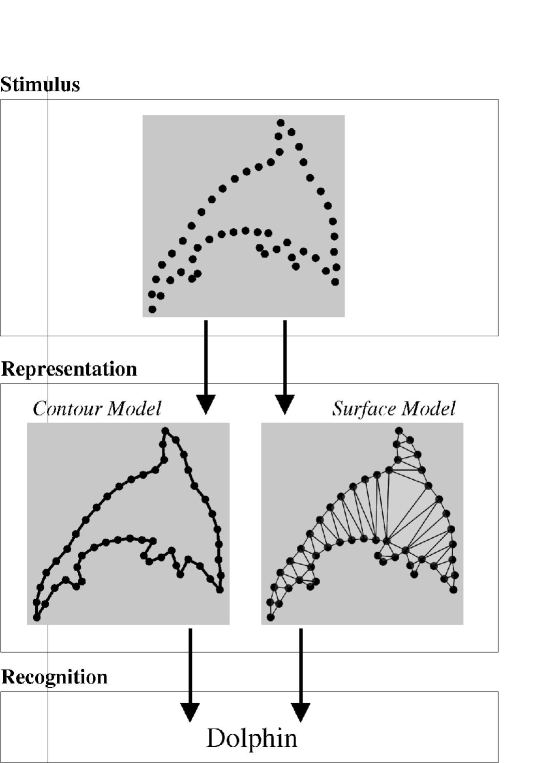
The hypothesis we formulated for the question is that when a set of cues is presented, we tried to form a surface that fits the set of cues. Directional information can help the process but is not necessary. Without it, we are still capable of performing the task of grouping non-directional cues. Figure 1 illustrates the two views: contour based and surface based. The contour model is a more conventional approach to the grouping problem, and the surface model is our hypothesized approach. Given a well-organized set of primitives such as the one shown at the top, we can no doubt recognize the object as indicated at the bottom. In this case, the underlying shape is a dolphin. The exact computational steps to reach from the cues to the recognition are largely unknown. Nevertheless, it is safe to assume that we construct some internal representation, as we often experience such grouping precepts[19, 20]. The contour model considers a sequence of cues as the representation, while the surface model considers a surface (height fields) derived from the cues. In a sense, the surface model is more general than the contour model, as we can always derive a contour representation as a level set of the surface. On the other hand, we cannot derive a surface from a contour unless the contour forms a closed cycle. In such case, a surface can be derived from the contour as a subsequent fill-in process [21, 22].

Computationally, the two models shown in Figure 1 face different issues. For the contour model, the issue is to find a permutation of cues, with which a complete contour can be drawn. This is the contour integration problem. For the contour model to be a feasible one to account for the path from cues to recognition, an efficient and reliable contour integration method needs to exist, and a large number of algorithms have been proposed for the problem [23, 24, 25, 26, 27, 28, 29, 30, 31, 32, 33]. However, none has been shown satisfactory to account for the performance of the human perception. Furthermore, as stated above, most algorithms require directional information embedded in the cues, and cannot handle cases like the one shown in Figure 1.

For the surface model, we can fit a surface from a set of dots by using a standard triangulation algorithm such as Delaunay triangulation [34]. Then, the issue is to differentiate those triangles inside the boundary from those outside. For such surface model to be a feasible one, an efficient and reliable triangle differentiation method needs to exist. We conjecture that such method exists, thus the internal representation consists of two phases: straight triangulation of cues, and triangulation after the differentiation.

To study plausibility of our hypothesis, we conduct two studies: cognitive one and computational one. For the cognitive study, we divide subjects into three different cohorts. One was presented a set of dots representing a contour of a shape and the other two were presented a set of triangles representing the surface of the shape. The dot representation is the simplest representation of the underlying shape. According to our hypothetical model, the dot representation is converted internally to a surface representation. Furthermore, the surface representation evolves in two steps: all triangles resulted from triangulation of dots and triangles that are inside the underlying shape. Two triangle based representations provide the two respective internal representations. If our hypothetical model is correct, we expect to observe similar recognition performance in all three cohorts.

For the computational study, we design a simple algorithm that takes triangulation of dots and separates outer triangles from inner ones. This process will bring grouping of visual cues as detailed in Method Section. We also design another algorithm that uses the grouping result to retrieve the shape from the database of shapes. This retrieval procedure allows us to compare the performance of the computational approach with the above cognitive study. If an algorithm using the surface based model outperforms a contour based algorithm of similar computational complexity, the evidence favors the surface based hypothesis over the contour based one. Furthermore, if the performance of the surface based algorithm is comparable to the human performance, the evidence favors the surface based model.

In the followings, we use bold capitals (P) for sets, bold letters (x) for 2D structures such as points and triangles, Greek letters ($\phi$, $\Omega$) for functions and transformations, and italic alphabets ($K$, $n$) for scalar variables. We use shape to mean the boundary of an object. We only consider shapes that are connected and have no holes. Thus, a shape forms a connected simple cycle (i.e. a connected cycle without self-intersection).

Figure 1: Surface model vs. contour model. The Top image is a visual stimulus shown to a subject, and the two middle pictures represent the two internal models that may be constructed internally to induce the recognition.

2 Methods

2.1 Experiment 1 (Cognitive Study)

Twenty subjects (10 male and 10 female) from Susquehanna University, both undergraduate students and staff members, with normal or corrected to normal vision participated in the study. The experiment complies with the Code of Ethics of the World Medical Association (Declaration of Helsinki) for experiments involving humans and was approved by the Institutional Review Board of Susquehanna University prior to its implementation.

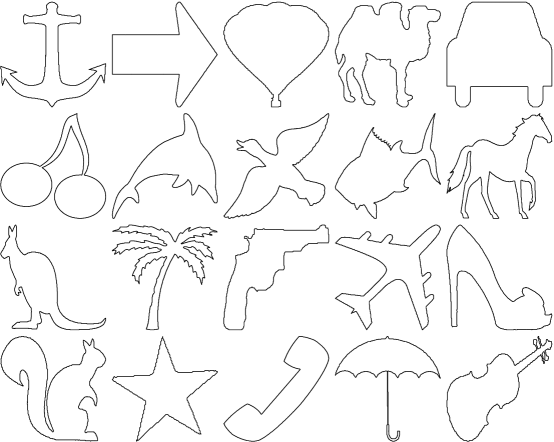
The experiment was conducted in a computer lab lit by fluorescent lighting. Each subject was seated in front of a personal computer with a 17-inch monitor. All visual stimuli were images with 512 by 512 pixels and displayed on a 5.6 by 5.6 $cm^{2}$ window in the monitor. Twenty shapes of animals and objects shown in Figure 3 were used in the experiments. They were represented by a densely populated sequence of points denoted by S. A computer program written in Processing programming language took S and generated visual stimulus. In addition to S, the program required the number of sampled points ($K$).

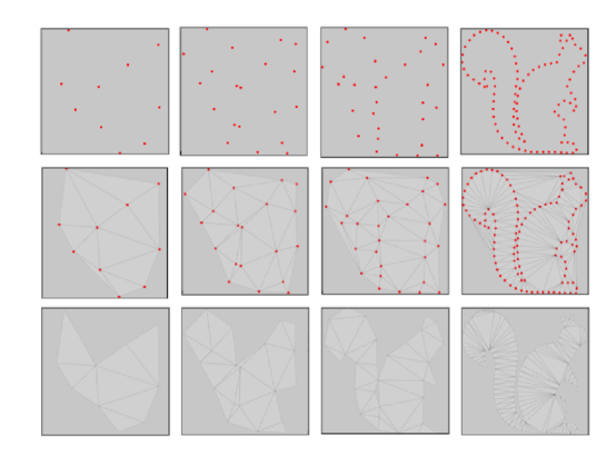
The program can generate three types of representations: Points representation, Triangle representation, and All-Triangle representation. Let $\Omega_{P}$, $\Omega_{T}$, and $\Omega_{A}$ denote the Point, Triangle, and All-Triangle representations, respectively. For $\Omega_{P}$, the program simply samples S uniformly into $K$ sampled points denoted as P, and then displays them on the window using red disks of 10 pixel radius. For $\Omega_{A}$, the program first prepares $\Omega_{P}$, and then runs Delaunay triangulation on P. It then displays both points and triangles. Points are shown with red disks of 10 pixel radius, faces of triangles are shown in lighter shade of gray than the background, and the sides of the triangles are shown in slightly darker shade of gray than the background. For $\Omega_{T}$, the program first prepares $\Omega_{A}$. For each triangle, the program checks if the center of the triangle (the average of the three vertex coordinates) is inside the shape. If not, the triangle is removed. The program then displays only the remaining triangles using the same shades used in $\Omega_{A}$. Figure 2 shows examples of $\Omega_{P}$, $\Omega_{A}$, and $\Omega_{T}$ for a squirrel shape at $K=10$, 20, 30, and 100.

Among the twenty participants, 8 were shown $\Omega_{P}$, 6 were shown $\Omega_{A}$, and 6 were shown $\Omega_{T}$. Each participant went through all twenty shapes in a random order, but viewed them only in the particular representation of the group. At the beginning of viewing of a shape, $K$ is set to 10. Thus, the $\Omega_{P}$ group saw 10 small disks at the 10 sample points. The $\Omega_{A}$ group saw 10 disks and its Delaunay triangulation. The $\Omega_{T}$ group saw a set of triangles in the Delaunay triangulation whose centroids were inside the shape delineated by the 10 sample points.

At $K=10$, most shapes are not recognizable. The participants were allowed to increase $K$ at 10 increment by hitting the SPACE bar. They were asked to increase $K$ until they were able to recognize the shape shown by the particular representation. At the time, they were asked to hit another key (’d’), which brings a dialog with a list of shapes. They were asked to select the recognized shape from the list. If no appropriate shape was found in the list, the participants were able to go back to the experiment and continue from the point where they were left off. The participants were not able to reduce the number of points. The program recorded both $K$ at the time of recognition and the selected shape. The list in the dialog remained the same throughout the experiment and provides names of 20 shapes used in the experiment.

Figure 2: Sample images of stimuli used in Experiment 1. Each row shows a particular representation, and each column shows images at different sample size ($K$). Row 1: ”Points”($\Omega_{P}$), Row 2: ”All Triangles”($\Omega_{A}$), Row 3: ”Triangles”($\Omega_{T}$). Column 1: $K=10$, Column 2: $K=20$, Column 3: $K=30$, Column 4: $K=100$.

Figure 3: Shapes used in our experiments.

2.2 Experiment 2 (Computational Study)

In this section, we describe two dot grouping algorithms, one surface based and the other contour based. We use them to compare their performance in reconstructing the original shape. We then describe a shape retrieval algorithm using the surface based grouping. We use it to compare the algorithmic retrieval against the results of the first experiment.

We first describe a grouping algorithm with the surface based representation, which differentiates triangles inside a shape and those outside the shape. We do this by exploring a planar Hamiltonian cycle of the points from which the triangulation is derived. The overall strategy is the following. Let $\textbf{P}=[\textbf{p}_{1},\textbf{p}_{2},\cdots,\textbf{p}_{K}]$ be the set of points in the order that delineates the shape. Some of the points are at the boundary of the triangulation, which we can sequence. Let $\textbf{B}=[\textbf{b}_{1},\textbf{b}_{2},\cdots,\textbf{b}_{k}]$ be the sequence of boundary points. For simplicity and without loss of generality, assume both P and B are given in the clockwise order around the shape.

We can show that the order of points in B is preserved in P. In other words, take a pair of adjacent points in B (with possible wrap around), say $\textbf{b}_{i}$ and $\textbf{b}_{j}$, and find the corresponding points in P, say $\textbf{p}_{i^{\prime}}=\textbf{b}_{i}$ and $\textbf{p}_{j^{\prime}}=\textbf{b}_{j}$. Then, no other points from B can appear in the clockwise path from $\textbf{p}_{i^{\prime}}$ to $\textbf{p}_{j^{\prime}}$ in P. This is so, because a triangulated graph of triangulation is planar and violation of the above property results in a non-planar Hamiltonian path. The property allows us to refine B by removing some outer triangles and exposing points that are missing in B. When all points are exposed, we obtain a planar Hamiltonian cycle of the point set. Of course, we do not know the sequence in P, thus which triangle to remove. However, observing Figure 2, it appears that we can use some heuristics to differentiate those outside the shape and those inside. More specifically, those triangles that are outside the shape tend to be ’flat’. This trend becomes more prominent as the sample size ($K$) increases since one side of a triangle which connects adjacent pair of points in the shape decreases while the other two which connect non-adjacent pairs remain relatively unchanged.

What we need is a measure of flatness. Empirically, we found the following effective. We denote a boundary edge connecting points x and y as $(\textbf{x},\textbf{y})$. Since a boundary edge is part of a single triangle in the triangulation, we can uniquely associate the edge with the other vertex of the triangle. Let the other vertex denoted as xy. Then the flatness of $(\textbf{x},\textbf{y})$ is defined as

$$\phi(\textbf{x},\textbf{y})=\|\textbf{x}-\textbf{y}\|-\min(\|\textbf{x}-\textbf{y}\|,\|\textbf{x}-\textbf{xy}\|,\|\textbf{y}-\textbf{xy}\|)$$ (1)

where $\|\textbf{x}-\textbf{y}\|$ is the length of the edge $(\textbf{x},\textbf{y})$. In other words, the flatness of a boundary edge $(\textbf{x},\textbf{y})$ is the length of the edge minus the shortest side of the triangle associated with $(\textbf{x},\textbf{y})$. Note that we can remove a boundary edge $(\textbf{x},\textbf{y})$ only if xy is not at the boundary (or if it is internal). Else, the trace of the boundary points will not be a simple cycle. We call a boundary edge $(\textbf{x},\textbf{y})$ removable, if xy is internal.

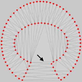
See Figure 4 for illustration. A Hamiltonian cycle of the shape is delineated in red. Starting from the top-left vertex, the order of the cycle is enumerated. There are 8 boundary edges, which are shown with thicker lines. Among 10 vertices, 8 are currently at the boundary of the triangulated surface. They are shown with red disks. There are two internal vertices and they are shown with blue disks. Thus, $\textbf{B}=[\textbf{b}_{1},\cdots,\textbf{b}_{8}]$ is $[\textbf{p}_{1},\cdots,\textbf{p}_{6},\textbf{p}_{9},\textbf{p}_{10}]$ or its circularly rotated version. Currently, there are 4 removable edges. They are shown with dashed lines. Consider the removable edge at the bottom of the figure and let the two vertices x and y. Then, $\textbf{xy}=\textbf{p}_{8}$. At this point, $(\textbf{x},\textbf{y})$ has the largest flatness measure among the four removable edges. After $(\textbf{x},\textbf{y})$ is removed, $(\textbf{p}_{2},\textbf{p}_{3})$ and $(\textbf{p}_{9},\textbf{p}_{10})$ are no longer removable. Instead, we have two removable edges: $(\textbf{p}_{6},\textbf{p}_{8})$ and $(\textbf{p}_{5},\textbf{p}_{6})$. We will recover the Hamiltonian cycle shown in red by removing $(\textbf{p}_{6},\textbf{p}_{8})$. We will recover a different Hamiltonian cycle by removing $(\textbf{p}_{5},\textbf{p}_{6})$.

Figure 4: An illustration of a triangulated graph and notations used. Edges in red delineate the shape. Dashed edges are removable. Red vertices are on the boundary of the current triangulated graph. Blue vertices are internal. For each boundary, there is a unique triangle associated with it.

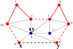
Note that the flatness measure captures the heuristic described previously. If x and y are adjacent pair, $\lim_{K\rightarrow\infty}\|\textbf{x}-\textbf{y}\|=0$. Thus, $\lim_{K\rightarrow\infty}\phi(\textbf{x},\textbf{y})=0$. On the other hand, when x and y are not adjacent pair, but either x and xy or y and xy is, then $\lim_{K\rightarrow\infty}\|\textbf{x}-\textbf{y}\|>0$ and either $\lim_{K\rightarrow\infty}\|\textbf{x}-\textbf{xy}\|=0$ or $\lim_{K\rightarrow\infty}\|\textbf{y}-\textbf{xy}\|=0$. Thus, $\lim_{K\rightarrow\infty}\phi(\textbf{x},\textbf{y})>0$. The remaining case is when none of $(\textbf{x},\textbf{y})$, $(\textbf{x},\textbf{xy})$, and $(\textbf{y},\textbf{xy})$ are adjacent. This case is rare but can happen around a concave part of the shape. We claim that, in this case, $\|\textbf{x}-\textbf{y}\|$ tends to be the largest among the three sides of the triangle. Thus, $\phi(\textbf{x},\textbf{y})>0$. This is because Delaunay triangulation prohibits a point to be inside the circumscribing circle of any triangle. When $\|\textbf{x}-\textbf{y}\|$ is the largest, the center of the circumscribing circle will be situated away from the shape. Then, it has good chance that no parts of the shape are inside the circle. When $\|\textbf{x}-\textbf{y}\|$ is not the largest, the center of the circumscribing circle will be situated toward the shape. Then, it has good chance that some parts of the shape are inside the circle. As $K$ increases, a point from such part will be sampled, and the triangle will be eliminated from the triangulation. Of course, we can carefully construct a shape where $\|\textbf{x}-\textbf{y}\|$ is the smallest, yet the circumscribing circle never crosses the shape. For example, see Figure 5. A large triangle with the arrow in it persists as $K$ increases while the edge at the base of the triangle has the flatness of 0. In such cases, we need a tie-breaker that choose an edge with non-adjacent points over those with adjacent ones, because both have the flatness of 0. The length of the boundary edge is a possible tie-breaker as it remains relatively unchanged as $K$ increases while a boundary edge formed by adjacent points approaches zero. Using the tie-breaker, we can indeed remove the edge and successfully extract the complete shape of Figure 5. However, since shapes like the one shown in Figure 5 is rare, we do not explore such option in our experiments and keep the flatness measure to the simple form of (1).

Figure 5: An example shape that may be problematic for Algorithm 1. The edge pointed by the arrow, when it becomes a boundary edge after triangles below it are removed, will have the flatness of 0. Since the circumscribing circle of the associated triangle (the large one with the arrow in it) does not cross the shape, the triangle persists regardless of $K$. Thus, the flatness of the boundary edge remains 0, which makes removing it based on the flatness measure problematic.

Now, we describe an algorithm to remove triangles outside the shape using the flatness measure of (1). We want to do it in a determinant fashion so that we can easily reproduce the results. We want to do it in a computationally efficient and simple manner so that the performance is impacted by the representation and not by sophisticated search and optimization techniques. More specifically, we limit ourselves to a polynomial algorithm without any backtracking. This led to a greedy algorithm shown in Figure 1.

Note that Delaunay triangulation of $K$ points takes $O(K\log K)$. There are $O(K)$ edges in the triangulation, thus collecting removable boundary edges takes $O(K)$ and sorting them takes $O(K\log K)$. Since each edge is visited at most once in the while loop and insertion of edges into the sorted list takes $O(\log K)$, the loop takes $O(K\log K)$. Sequencing the boundary points takes $O(K)$. Thus, the overall complexity of the algorithm is $O(K\log K)$. Note that $(\textbf{x},\textbf{y})\in\textbf{E}$ can change from removable to unremovable since removing another edge can expose xy. Also, $(\textbf{x},\textbf{xy})$ or $(\textbf{y},\textbf{xy})$ may not be removable when they are inserted in E. We could check the removable condition before adding them to E to speed up the computation slightly. We did not do so in the algorithm to keep it simple, as it does not affect the overall complexity.

Input: P: a (non-sequenced) set of sample points

Output: B: a sequenced series of boundary points

1 Triangulate P

2 Collect removable boundary edges and store them in E.

3 Sort edges in E according to (1) in the descending order.

4 while $\textbf{E}\neq\emptyset$ do

5       Pop $(\textbf{x},\textbf{y})$ from E

6       if xy is internal then

7             Insert $(\textbf{x},\textbf{xy})$ and $(\textbf{y},\textbf{xy})$ to E according to (1).

8            

Sequence the boundary points.

Algorithm 1 Algorithm1: Surface-based Grouping Algorithm

Next, we design a similar grouping algorithm for the contour based model. As stated in Introduction, most contour based grouping algorithms require tangential and/or curvature information, thus are not applicable for our purpose. By the same reasoning to keep our surface based algorithm simple, we want a simple algorithm that is not heavily dependent on optimization and elaborate searching. We decided to use a Minimum Spanning Tree (MST) to group sampled points using the proximity information. Basically, we form a graph in which sampled points are vertices and every pair of vertices is connected by an edge whose weight is set to the Euclidean distance between the vertices. We then apply Kruskal’s MST algorithm to find an MST [35]. A straightforward implementation of Kruskal with a fully connected graph has the computational complexity of $O(K^{2}\log K$).

One issue of an MST is that it can have branches, thus we may not be able to translate the tree into a simple cycle easily. Instead of comparing two methods based on the extracted shape, we use edges selected by them to score the performance. The original shape can be represented by $K$ edges that links adjacent points. Each method yields a set of edges: at most $K$ edges for the surface based one and $K-1$ for the contour based one. We use the proportion of edges that are in the original shape as the performance measure. More precisely, the grouping score denoted as $\xi$ is defined as

$$\xi\left(\textbf{E}_{K}\right)=\frac{|\textbf{E}_{K}\cap\textbf{E}(\textbf{P})|}{|\textbf{E}_{K}|}$$ (2)

where $\textbf{E}_{K}$ is a set of boundary edges for the surface based method and a set of MST edges for the contour based method at the sample size of $K$, $\textbf{E}(\textbf{P})$ is a set of edges formed by connecting every circularly adjacent points in P, and $|\textbf{E}|$ gives the number of edges in E. Note that $\textbf{E}(\textbf{P})$ has $K$ edges, delineates the original shape, and serves as the ground truth in the measure.

Note that the contour based method benefits more by this measure. The number of edges in an MST is $K-1$ instead of $K$, thus a result with the perfect score of 1 still does not extract the entire shape. More importantly, the MST often has branches, which results in a perceptually unacceptable interpretation of the shape. Yet, it may result in a high score. For the surface based one, the solution is always a simple cycle, and the quality of the solution and the performance measure typically match up well.

The second part of the study is to investigate how the grouping performance of the algorithms compare to the recognition performance presented in Experiment 1. To do so, we need to build a shape retrieval algorithm on top of the grouping result. There have been many algorithms to retrieve a shape from a database using contour features. Earlier ones only allow rigid transformation on the contour [36, 37]. For an extensive review, see [38]. More recent ones allow non-rigid transformation and partial occlusion [39, 40, 41]. Since our goal is not to develop a full-fledged shape retrieval system, we keep the shape retrieval algorithm simple. We decided to use DC-normalized Fourier descriptors computed on centroid distances as the contour features [42] and use the Euclidean distance in the feature space for a similarity measure between features.

The DC-normalized Fourier descriptors are obtained from a sequence of points delineating the shape by first computing the distance from the centroid of the sequence of points to each point, computing the Fourier coefficients of the real valued distance values, taking the absolute value of each complex valued Fourier coefficient, and then dividing each absolute coefficient by the DC component. We divide each coefficient by the DC component so that the descriptors are scale invariant. We use the centroid distance as it is shown more effective than the raw coordinate [43].

Using the DC-normalized Fourier descriptors, we compute the sample size needed to retrieve each reference shape from the collection of 20 shapes. Figure 2 summarizes the retrieval algorithm. It takes the database of shapes ($Db$) and an index ($id$) to a reference shape in the database. We pre-compute the DC-Normalized Fourier descriptors for each shape $\textbf{Z}_{i}$ and store them in the database. We only store 10 coefficients corresponding to the 10 lowest frequency components, as they tend to capture the principle structures of the shape while higher frequency components tend to capture perturbation, noise, and artifacts.

The algorithm loops over $K$ from 30 at increment of 10, like in Experiment 1 (Line 1). Since we need at least 21 sample points to collect 10 DC normalized Fourier coefficients, we start from 30 instead of 10 as in Experiment 1. For each $K$, we sample the shape (Line2), apply Algorithm1 to extract a sequence of boundary points (Line 3), and compute 10 Fourier descriptors (Line 4) using the boundary points. We compare the descriptors with those in the database using a simple Euclidean distance (Lines 5-6). Note that $|Db|$ in Line 5 gives the cardinality of the database (20 in our case). We deemed the shape is retrievable if the Euclidian distance of the correct shape ($s_{id}$) is the smallest and the next smallest is at least 3 times larger. (Line 7). As soon as the shape becomes retrievable, the algorithm returns the sample size denoted as $n$ (Line 8). Although the algorithm always terminated in our experiments, the termination condition may never be met if two shapes in the database are very similar. In this simple implementation, we do not worry about such situation. The algorithm mimics the behavior of a careful human observer who commits to an answer only when he/she is very certain about the choice (three times more than the other shapes).

Input: $Db=\left\{\left(\textbf{S}_{i},\textbf{Z}_{i}\right)\right\}$: the shape database with both shapes and Fourier descriptors.

Input: $id$: a reference shape id

Output: $n$: Retrievable sample size

1 foreach $n=30,40,50,\cdots$ do

2       P=Sample $n$ points from $\textbf{S}_{id}$

3       B=Algorithm1(P)

4       $\textbf{x}=FourierDescriptorsOf(\textbf{B},10)$

5       for i=1 to $|Db|$ do

6             $s_{i}=\|\textbf{x}-\textbf{Z}_{i}\|$

7            

8      if $s_{id}=\min_{i}(s_{i})$ and $\min_{i\neq id}\left(s_{i}/s_{id}\right)>3$ then

9            return $n$

Algorithm 2 Algorithm2: Shape retrieval algorithm

Unfortunately, the above algorithm is not applicable to the contour based grouping, which gives a tree not a shape. In order to derive some meaningful quantities associated with the contour based approach, we devise another way to relate the grouping performance to a retrieval one. For each shape, we examine grouping results at various $K$. We start from $K=10$ and increase $K$ at 10 increment until $K=200$. For each $K$, we evaluate the grouping score, $\xi$, defined previously. Then, we find a point in $K$ denoted as $m$ after which the grouping score remains above 80%. The underlying assumption is that shape retrieval becomes trivial when the grouping accuracy reaches a certain level. We chose 80% empirically but observed that the overall result was not sensitive to the choice. With this measure, we can compare the contour based algorithm with the human performance as well as the surface based algorithm.

3 Results

3.1 Experiment 1

Among six participants in the $\Omega_{T}$ group, two did not use SPACE bar at all and guessed the shape from the initial representation at $K=10$. Their guesses were almost all incorrect, and therefore, we excluded their results in our analysis. Other participants answered most shapes correctly. We did not remove occasional incorrect answers from our results, because answering ’fish’ instead of ’dolphin’ or ’plane’ instead of ’duck’ shows some degree of recognition. Thus, there are 8 participants in $\Omega_{P}$ group, 6 in $\Omega_{A}$ group, and 4 in $\Omega_{T}$ group, and each participant has 20 data points.

The mean and the standard deviation of $K$ for each group and shape are listed below in Table 1. In general, $\Omega_{T}$ has the smallest mean, followed by $\Omega_{P}$, and $\Omega_{A}$ having the largest mean. According to the Kruskal-Wallis test, the representation of shapes affected the response time significantly ($H(2)=43.16$, $p<0.01$).

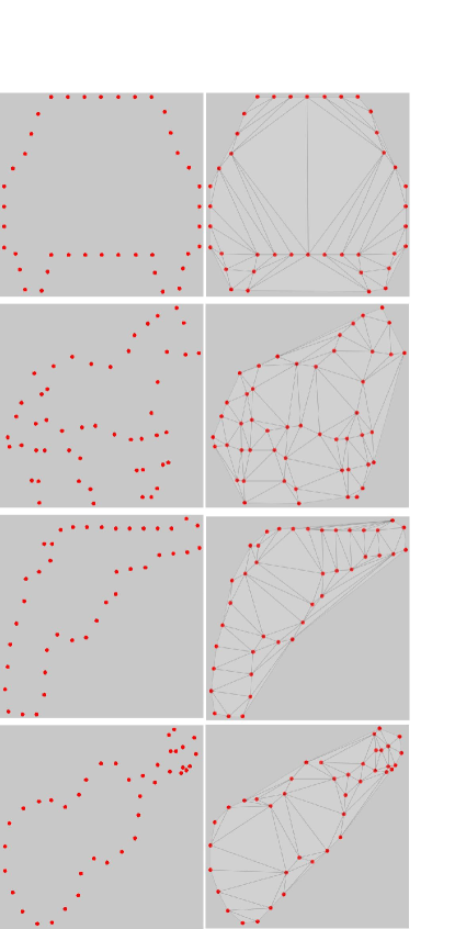
Next, we investigate more closely how recognition of each shape is affected by different representations. Table 2 shows p-values of pooled t-test between $\Omega_{P}$ and $\Omega_{A}$, and $\Omega_{P}$ and $\Omega_{T}$, treating $\Omega_{P}$ as the control group. Those entries with $p<0.05$ are shown in bold. There are four shapes in $\Omega_{P}$ vs. $\Omega_{A}$ column that are $p<0.05$. Figure 6 shows these four shapes in $\Omega_{P}$ and $\Omega_{A}$ at $K$ near the mean value for $\Omega_{P}$. Between $\Omega_{P}$ and $\Omega_{T}$, seven shapes show significant difference. For six shapes out of the seven, $\Omega_{T}$ shows faster recognition than $\Omega_{P}$. An exception is the umbrella shape where the triangulation failed to represent accurately the handle of the umbrella, making the recognition of the shape difficult. In general, grouping provided by $\Omega_{T}$ facilitated recognition. The results also indicate that the triangulation retained the correct grouping of cues in most cases.

The results show that the representations affect recognition, which contradicts our initial hypothesis that our visual system groups a set of dots via triangulation. However, the results do not reject a more general surface based grouping hypothesis. Furthermore, the results suggest that our visual system does not depend exclusively on either points or triangles. If our recognition only uses points representation, adding triangles as in $\Omega_{A}$ would not have had any effect on recognition. If our recognition only uses triangles, the recognition time of all three representations would have been similar and our initial hypothesis would have not been rejected. Thus, the results only paint a more complex picture of our visual system that combines various cues to facilitate the processing, even at a very basic level of grouping of dots; some configurations of triangles facilitate and some distract the grouping process.

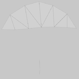
An interesting observation we were able to make was that recognition was often parts based. This is clear from the umbrella result of $\Omega_{T}$. Some participants were able to recognize the umbrella correctly at $K=20$. See Figure 7 for the image at $K=20$. At this point, only a small part of the pole/handle was visible and was disjoint with the canopy. Thus, in some cases, recognition came before reconstruction of the shape.

The part based recognition may be a reason for slow recognition of shapes shown in Figure 6. In these shapes, some important parts were obscured by triangles. For the Car shape, we think that wheels are important parts. In $\Omega_{A}$, they were obscured by clusters of similar triangles surrounding them. For the Horse shape, we think that legs are important parts. In $\Omega_{A}$, they were distracted by accidental alignment of triangles across legs. For the violin shape, we think that the body is an important part. In $\Omega_{A}$, it was obscured by triangles encompassing smoothly over the entire instrument. For the pistol, we think that the trigger and the hammer are important parts. In $\Omega_{A}$, they were obscured by clusters of nearby triangles.

Table 1: Mean sample size at recognition of shapes ($K$) for each representation and each shape.

	$\Omega_{P}$		$\Omega_{A}$		$\Omega_{T}$
Shape	Mean	Std	Mean	Std	Mean	Std
Anchor	32.50	6.61	36.67	14.91	22.50	5.00
Arrow	31.25	11.66	33.33	9.43	20.00	0.00
Balloon	37.50	15.61	35.00	12.58	25.00	10.00
Camel	43.75	15.76	65.00	23.63	42.50	5.00
Car	40.00	5.00	63.33	11.06	52.50	20.62
Cherries	41.25	9.27	51.67	13.44	45.00	17.32
Dolphin	40.00	8.66	31.67	3.73	20.00	0.00
Duck	40.00	10.00	48.33	12.13	35.00	17.32
Fish	45.00	18.71	43.33	7.45	22.50	5.00
Horse	45.00	8.66	61.67	14.62	37.50	5.00
Kangaroo	58.75	9.27	56.67	13.74	35.00	17.32
Palm tree	61.25	7.81	56.67	7.45	37.50	5.00
Pistol	42.50	7.07	86.67	24.27	45.00	19.15
Plane	41.25	8.35	46.67	9.43	35.00	12.91
Shoe	33.75	4.84	36.67	7.45	22.50	5.00
Squirrel	46.25	9.92	50.00	5.77	32.50	9.57
Star	23.75	6.96	30.00	11.55	15.00	5.77
Telephone	27.50	6.61	36.67	12.47	17.50	5.00
Umbrella	18.75	3.31	38.33	28.53	30.00	11.55
Violin	38.75	3.31	46.67	4.71	40.00	14.14
All	39.50	13.91	47.75	19.77	31.62	14.36

Table 2: p-values of Pooled t-tests for each shape in Experiment 1. Those less than 0.05 are shown in bold.

Shape	$\Omega_{P}$ vs $\Omega_{A}$	$\Omega_{P}$ vs $\Omega_{T}$
Anchor	0.53	0.03
Arrow	0.75	0.11
Balloon	0.77	0.20
Camel	0.09	0.89
Car	4e-4	0.12
Cherries	0.14	0.64
Dolphin	0.06	2e-3
Duck	0.22	0.55
Fish	0.85	0.06
Horse	0.03	0.17
Kangaroo	0.76	0.01
Palm tree	0.33	4e-4
Pistol	6e-4	0.93
Plane	0.30	0.33
Shoe	0.43	5e-3
Squirrel	0.46	0.05
Star	0.27	0.07
Telephone	0.13	0.03
Umbrella	0.10	0.03
Violin	0.01	0.81

Figure 6: Four shapes (Car, Horse, Pistol, and Violin) whose results were significantly different between $\Omega_{P}$ (Left) and $\Omega_{A}$ (Right).

Figure 7: An example of parts based shape recognition. At $K=20$, parts are clearly disjoint. However, some participants were able to recognize the shape (Umbrella) correctly.

4 Experiment 2

First, we compare the performance score $\xi$ defined in (2) between the surface based algorithm and the contour based one at different $K$. Figure 8 shows plots of the mean score over 20 shapes at $K=30,40,\cdots,200$. The accompanying error bars are the standard error of the mean. Clearly, the surface based method consistently provides more accurate grouping of cues than the contour based one.

Figures 9 and 10 show instances of shape extraction at $K=50$ with the surface based approach and the contour based approach, respectively. Results of 20 shapes are shown. In each figure, sample points are shown with red dots, and the grouping result is shown with blue lines. In Figure 9, the triangulation of the sample points is also shown with dashed lines. The number above each figure is the value of $\xi$. The surface based method was able to find a Hamiltonian cycle on 19 shapes out of 20. One exception was the palm tree shape. As stated in Method Section, the contour based method, which finds a minimum spanning tree, often finds a tree with branches, making translation of the tree into a simple cycle difficult.

The surface based method showed difficulty dealing with a shape with thin structures. This is largely due to Delaunay triangulation’s preference toward fat triangles over thin ones. This characteristic is evident in the handle of Umbrella shape and the stems of Cherry shape. The Cherry shape actually contain two objects (two cherries), which poses another problem; Algorithim1 at the current form is not capable of dealing with multiple objects.

Figure 8: Performance comparison between the surface based and contour based grouping algorithms. Mean values of $\xi$ over 20 shapes are plotted at different $K$. The error bars are standard error of the mean.

Figure 9: Results of the surface based grouping algorithm at $K=50$. Edges selected are shown in blue. Dashed gray edges show triangulation. The number at the top of each result is the value of $\xi$.

Figure 10: Results of the contour based grouping algorithm at $K=50$. Edges selected are shown in blue. The number at the top of each result is the value of $\xi$.

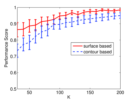
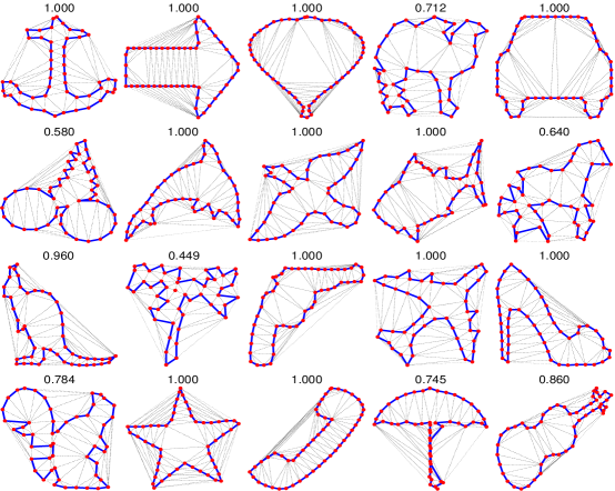
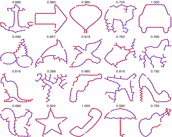
Table 3 shows the retrievable sample size $n$ and $m$ for each shape and for each grouping method (surface based and contour based ones). Note that $n$ is the result of Algorithm 2 shown in Figure 2, and $m$ is the sample size that guarantees 80% grouping accuracy as described in the Method Section. Algorithm 2 is not applicable to the contour based results.

Table 4 shows Pearson correlation coefficients and their p-values between an algorithmic performance measure ($n$ and $m$) and a mean recognition speed as reported in Table 1 with various representation types ($\Omega_{P}$, $\Omega_{A}$, and $\Omega_{T}$). Note that $n$ of the surface based method has highest correlation among the three algorithmic ones with all types of the human retrieval performance.

Table 3: The results of the shape retrieval studies. $n$ is the result of the surface based retrieval algorithm (Figure 2), which is not applicable to the contour based approach. $m$ is the minimum sample size that guarantees $\xi>0.8$.

	Surface		Contour
	n	m	n	m
Anchor	30	30	-	50
Arrow	30	30	-	30
Balloon	30	30	-	30
Camel	110	70	-	80
Car	30	30	-	30
Cherries	150	120	-	90
Dolphin	30	30	-	40
Duck	50	30	-	30
Fish	30	30	-	70
Horse	120	130	-	180
Kangaroo	40	30	-	50
Palm tree	150	100	-	140
Pistol	30	30	-	30
Plane	30	30	-	50
Shoe	30	30	-	60
Squirrel	120	60	-	70
Star	30	30	-	40
Telephone	30	30	-	30
Umbrella	70	60	-	200
Violin	40	30	-	60
Mean	59.00	48.00	-	68.00

Table 4: Correlation between algorithmic retrieval performance and mean recognition speed of humans. Shown are Pearson correlation coefficient with its p-value inside parentheses. The correlation is taken between the mean column ($\Omega_{P}$, $\Omega_{A}$, and $\Omega_{T}$) in Table 1 and each column (surface $n$, surface $m$, and contour $m$) in Table 3.

	Surface		Contour
	n	m	n	m
$\Omega_{P}$	0.42 (0.06)	0.31 (0.18)	-	0.04 (0.86)
$\Omega_{A}$	0.34 (0.14)	0.16 (0.32)	-	0.13 (0.59)
$\Omega_{T}$	0.44 (0.05)	0.40 (0.08)	-	0.19 (0.40)

5 Discussion

The results of Experiment 1 showed that triangulation can sometimes distract recognition. Thus, the results did not support our original conjecture. However, it is still possible that we employ triangulation as an internal representation at a subconscious level. Then, the representation would not distract our recognition. Also, the results only concern triangulation based representation, and do not reject a more basic hypothesis of surface based interpolation. Maybe, triangulation is too ”artificial” and our perception employs a more flexible and smoother interpolation scheme. The surface based representation does offer various computational advantages over the contour based one as demonstrated in Experiment 2.

Removal of outer triangles ($\Omega_{T}$) enhances recognition while inclusion of outer triangles ($\Omega_{A}$) hinders recognition. By removing outer triangles, $\Omega_{T}$ provides explicit grouping information that is not available in $\Omega_{P}$ nor $\Omega_{A}$. $\Omega_{A}$ does contain all the information that is present in $\Omega_{P}$. It also contains some ’noise’ in the form of outer triangles. Our experiment showed that the noisy information sometimes distracts viewers.

The results of Experiment 2 support utility of the surface based grouping. A simple greedy algorithm proposed in this paper successfully reconstructed 12 shapes perfectly out of 20 with 50 sample points (See Figure 9). On the other hand, a similar contour based approach could recover only two shapes (Figure 10). The superior performance of the surface based approach is the result of restricting a solution to a simple cycle one. The approach effectively recovered a Hamiltonian cycle in 19 shapes out of 20. Notable disadvantages of the surface based approach at the current form are that it has difficulty in extracting thin parts, and is not applicable to separate multiple objects.

Delaunay triangulation constructs a planar graph and reduces the number of edges in the fully connected graph from $O(K^{2})$ to $O(K)$. The reduction of edges facilitated grouping, yet did not degrade the performance. Thus, Delaunay triangulation effectively retained the underlying shapes in our experiments. This is true for ’fat’ objects but may not be so for ’thin’ objects.

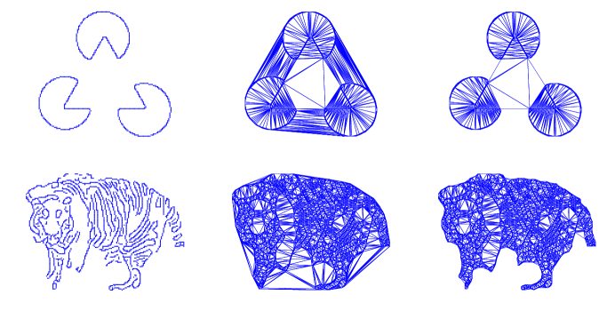
Another advantage of the surface based approach is that it tends to delineate illusory contours. Consider a problem where we are given a set of edge points resulted from some edge detector [3, 4] applied to an image with an object. Our goal is to group these points into a coherent shape outlining the boundary of the object. Since some edge points represent patterns inside the object, the solution may not be a Hamiltonian. Thus, instead of forcefully searching for a Hamiltonian solution as in Figure 1, we stop the search when there is no boundary edges that are ’sufficiently’ flat. We set the sufficiency to be 5 for our illustration. Results of applying this modified algorithm to an edge image of a Kanizsa triangle and another edge image with a tiger are shown in Figure 11.

As the results show, the modified algorithm was able to produce an illusory Kanizsa triangle. It was also able to group disjoint groups of edge points at the tail of the tiger and interpolate end points of occluded strip patterns on the body of the tiger. These grouping tasks are rather difficult computationally and various attempts have been made in the past[31, 44, 45] with highly elaborate schemes. The surface based approach allows such grouping to take place with a simple greedy approach. The results also show some limitations of triangulation based approach. In the Kanizsa triangle example, the pack-man shapes are abruptly cut instead of being interpolated smoothly to complete a disk. The triangle inside the illusory triangle is artificially produced and does not agree with our perception. We observed these issues in Experiment 1 where artificial lines resulted from triangulation can potentially distract recognition.

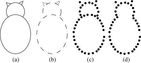
The surface based approach also makes sense from evolutional and ecological viewpoints, as the role of our vision is to infer the 3D structure of the environment. Using surfaces to construct the environment is more direct than using contours first and then interpolate. We can also point out via a simple drawing of Figure 12(a) that we interpret this drawing as a 3D figure rather than 2D drawing. In particular, we tend to see a bulge in both torso and head of the cat like figure. This perception persists when we introduce gaps as in Figure 12(b) replace contour fragments with isolated dots as in Figure 12(c), or further remove the occlusion boundary between the head and torso as in Figure 12(d).

One explanation is that we recognize a cat from the drawing and use our high-level knowledge of it to interpolate the surface. However, no living cat actually looks like this drawing. One may then argue that the drawing does not represent the actual cat but a conceptual model of it. However, unless there has been a link between this drawing to the actual cat, the conceptual model cannot be developed[46]. A more plausible explanation in our opinion is that this drawing although extremely simple (two ellipses and two triangles) has enough information for us to infer most plausible surface interpretation (perhaps in a Bayesian sense), which resulted both ellipses to have a bulge. Using the interpretation, we link it to a cat among all other things in our database, due to features present in the drawing including the bulge. Once this link is established, some features are further enhanced via the conceptual model derived from the high-level knowledge.

Figure 11: Application of the algorithm with a stopping condition of $\phi>5$. Left: Edge images obtained by Canny edge detector. Middle: Delaunay triangulation applied to the edge image. Right: Remaining triangles after boundary edges with $\phi>5$ are removed incrementally.

Figure 12: Why do we see a bulge? (a) A cartoon drawing of a cat. We tend to see a bulging 3D shape in both torso and head of this drawing. (b) The 3D perception tends to persist when gaps are introduced to the boundary, (c) edge fragments are replaced with small disks, or (d) the occlusion line is removed.

Artists have developed numerous techniques to induce 3D percepts in 2D drawings [47]. Their techniques demonstrate how easy it is to bring realistic physical constructs from a drawing. Figure 12(a) is one simple example. Gibbon’s ecological view suggests that a 3D view of a form is primary while a 2D view is acquired via training [46]. Koenderink’s catalog of surface interpretations from contours and their joints provide some clues as to why some features induce 3D percepts [20]. Tse proposed volume based grouping of contour fragments to account for amodal completion and extended the relatability proposal of Kellman and Shipley[48, 49]. However, there is no computational algorithm that groups a set of cues and renders 3D interpretation possible. Since our triangulation based approach did not agree with our perception, we need an alternate proposal.

So where can we go from here? We argue above that surface based grouping hypothesis should not be rejected. So we may just discredit triangulation based grouping hypothesis and contemplate other means of interpolation? Although our experiments rejected the Delaunay triangulation based interpolation hypothesis, we are hesitant to discount triangulation entirely. After all, realistic rendering of a 3D world has been possible using triangles alone, and computational efficiency and algorithmic simplicity associated with triangulation are too attractive to abandon easily. At this stage of our investigation, computational consideration is important as we want to be able to generate visual stimuli and test our proposals easily, consistently, and repeatedly.

By examining $\Omega_{A}$ and $\Omega_{T}$ representations of shapes, we feel that the main sources of distraction in them are triangles whose shapes are acutely different from others. Some triangles are quite large and some are thin. Our percept can be drawn to these salient triangles and gain sense of disjointness with a large triangle and coherency with a cluster of thin triangles. Thus, maybe a way to group isolated dots in a computationally efficient and perceptually agreeable manner is to use a more homogeneous set of triangles rather than Delaunay ones. One way to achieve such interpolation is to sub-divide a large triangle or a set of thin triangles by introducing new internal points. The approach is common for image synthesis of a parametric surface.

There are a number of advantages with this approach. First, by using triangles as the construction blocks, we can inherit some of advantages of the Delaunay based grouping algorithm, including its computational efficiency and simplicity, non-dependence on orientation and curvature information, and capability to form illusory contours. We can also use the Delaunay to draw an initial configuration, from which a more homogeneous configuration can be derived. Thus, implementation of the approach seems quite feasible. Second, we can achieve an arbitrary level of homogeneousness by applying the subdivision repeatedly. Thus, a smoother interpolation with more elaborate construction blocks can be approximated by the approach. Third, we may be able to use the representation to decompose a non-convex shape into convex parts. Then, we will be able to handle multiple objects, in which each object forms a convex shape but joined together into a non-convex outline. Polynomial-time algorithms have been known to decompose a non-convex polygon into a set of convex polygons [50]. The algorithms are not applicable here as there is a great amount of ambiguity in forming an outer polygon from a set of cues. (See Figures 10 and 9.) Another approach is to first compute the distance transform on an image lattice where each distance value tells the distance to the nearest cue [51]. Local maxima of the distance map gives convex cores, which can be used to group lattice points into a collection of convex sets. By having a uniform triangulation, we avail ourselves with a non-uniform lattice, which can be used to derive a distance map, which in turn can be used to separate multiple objects. Fourth, by setting a threshold value for filtering local maxima and decreasing it from a higher value to a lower one, we can construct a scale-space representation of a set of convex parts. Such representation has been shown effective in encoding both global and local information for object recognition. [52, 37].

6 Conclusion

The results of the cognitive study showed that shape recognition performance was dependent on the representations among dots, Delaunay triangles, and Delaunay triangles inside the shape. The results reject out initial conjecture that non-directional cues were grouped via Delaunay triangulation. The results of the computational study showed a number of advantages for the triangulation based grouping and recognition over contour based ones.

Our final thought on the problem of grouping non-directional visual cues is to further explore non-Delaunay triangulation, in particular adaptive triangulation that yields a representation comprised of visually similar triangles. We will be able to obtain such triangulation from Delaunay one by repetitive sub-division. We can then conduct cognitive experiments similar to the ones presented in this paper using the new triangulation.

References

- [1] Attneave, F.: Some information aspects of visual perception. Psychological Review 61(3) (1954) 183–193
- [2] Ullman, S.: High-level vision: object recognition and visual cognition. MIT Press, Cambridge, MA (1996)
- [3] Canny, J.F.: A computational approach to edge-detection. IEEE Transaction on Pattern Analysis and Machine Intelligence 8 (1986) 679–700
- [4] Marr, D.: Vision. W. H. Freeman and Company, San Francisco, CA (1982)
- [5] Elder, J.H., Zucker, S.W.: Computing contour closure. In: Proc. 4th European Conference on Computer Vision, Cambridge, UK (1996) 399–412
- [6] Sharon, E., Brandt, A., Basri, R.: Completion energies and scale. IEEE Trans. Pattern Analysis and Machine Intelligence 22(10) (October 2000) 1117–1131
- [7] Kimia, B., Frankel, I., Popescu, A.: Euler spiral for shape completion. International Journal of Computer Vision 54(1-3) (August 2003) 159–182
- [8] Aggarwal, J., Nandhakumar, N.: On the computation of motion from sequences of images: A review. Proceedings IEEE 76 (1988) 917–935
- [9] Horn, B., Schunck, B.: Determining optical flow: A retrospective. Artificial Intelligence 59(1-2) (January 1993) 81–87
- [10] Hoppe, H., DeRose, T., Duchamp, T., McDonald, J., Stuetzle, W.: Signed-distance field estimated from a set of unoriented noisy points. In: ACM SIGGRAPH. (1992) 71–78
- [11] Frankot, R., Chellappa, R.: A method for enforcing integrability in shape from shading algorithms. IEEE Transactions on Pattern Analysis and Machine Intelligence 10(4) (July 1988) 439–451
- [12] Julesz, B.: Textons, the elements of texture perception, and their interactions. Nature 290 (1981) 91–97
- [13] Bergen, J., Adelson, E.: Early vision and texture perception. Nature 333(6171) (1988) 363–364
- [14] Feldman, J.: Bayesian contour integration. Perception and Psychopysics 63(7) (2001) 1171–1182
- [15] Greene, E.: Recognition of objects displayed with incomplete sets of disrete boundary dots. Perceptual and Motor Skills 104 (2007) 1043–1059
- [16] Ommer, B., Mader, T., Buhmann, J.: Seeing the objects behind the dots: Recognition in videos from a moving camera. International Journal of Computer Vision 83(1) (June 2009) 57–71
- [17] Kovacs, I.: Gestalten of today: Early processing of visual contours and surfaces. Behav. Brain Research 82 (1996) 1–11
- [18] Field, D.J., Hayes, A., Hess, R.F.: Contour integration by the human visual system: Evidence for a local “association field”. Vision Research 33 (1993) 173–193
- [19] Humphrey, N.K.: The illusion of beauty. Perception 2 (1973) 429–439
- [20] Koenderink, J.J., van Doorn, A.J.: The internal representation of solid shape with respect to vision. Biological Cybernetics 32 (1979) 211–216
- [21] Elder, J.H., Zucker, S.W.: Evidence for boundary specific grouping. Vision Research 38(1) (1998) 143–152
- [22] Pessoa, L., Thompson, E., Noe, A.: Finding out about filling-in: A guide to perceptual completion for visual science and the philosophy of perception. Behavioral and Brain Sciences 21 (1998) 723–802
- [23] Arbelaez, P., Maire, M., Fowlkes, C., Malik, J.: Contour detection and hierarchical image segmentation. IEEE Trans. on Pattern Analysis and Machine Intelligense 33(1) (January 2011) 898–916
- [24] Cox, I.J., Rehg, J.M., Hingorani, S.: A baysian multiple-hypothesis approach to edge grouping and contour segmentation. International Journal of Computer Vision 11(1) (1993) 5–24
- [25] Grossberg, S., Mingolla, E.: Neural dynamics of perceptual grouping: Textures, boundaries, and emergent segmentation. Perception and Psychophysics 38(2) (1985) 141–171
- [26] Guy, G., Medioni, G.: Inferring global perceptual contours from local features. International Journal of Computer Vision 20(1) (1996) 113–133
- [27] Li, Z.: A neural model of contour integration in the primary visual cortex. Neural Computation 10(4) (1998) 903–940
- [28] Mahamud, S., Williams, L., Thornber, K., Xu, K.: Segmentation of multiple salient closed contours from real images. IEEE Trans. on Pattern Analysis and Machine Intelligence 25(4) (2003) 433–444
- [29] Papari, G., Petkov, N.: Adaptive pseudo dilation for gestalt edge grouping and contour detection. IEEE Transactions on Image Processing 17(10) (2008) 1950–1962
- [30] Parent, P., Zucker, S.W.: Trace inference, curvature consistency and curve detection. IEEE Trans. Pattern Analysis and Machine Intel. 11(8) (August 1989) 823–839
- [31] Saund, E.: Perceptual organization of occluding contours generated by opaque surfaces. CVPR 99 (1999)
- [32] Shashua, A., Ullman, S.: Structural saliency: the detection of globally salient structures of using a locally connected network. In: International Conference on Computer Vision. (1988) 321–327
- [33] Wang, S., Kubota, T., Siskind, J., Wang, J.: Salient closed boundary extraction with ratio contour. IEEE Trans. Pattern Analysis and Machine Intelligence 27(4) (April 2005) 546–561
- [34] de Berg, M., Cheong, O., van Kreveld, M., Overmars, M.: Computational Geometry: Algorithms and Applications. 1st edn. Springer (1997)
- [35] Cormen, T., Leiserson, C., Rivest, R., Stein, C.: Introduction to algorithms. MIT press (2001)
- [36] Asada, H., Brady, M.: The curvature primal sketch. IEEE Trans. on Pattern Analysis and Machine Intelligense 8(1) (January 1986) 2–14
- [37] Mokhtarian, F., Mackworth, A.: Scale based description and recognition of planar curves and two-dimensional shapes. IEEE Trans. Pattern Analysis and Machine Intelligence 8(1) (January 1986) 34–43
- [38] Zhang, D., Lu, G.: Review of shape representation and description techniques. Pattern recognition 37(1) (2004) 1–19
- [39] Sato, J., Cipolla, R.: Quasi-invariant parameterisations and matching of curves in images. International Journal of Computer Vision 28(2) (June 1998) 117–136
- [40] Sebastian, T., Klein, P., Kimia, B.: On aligning curves. IEEE. Trans. Pattern Analysis and Machine Intelligence 25(1) (January 2003) 116–124
- [41] Mio, W., Srivastava, A., Joshi, S.: On shape of plane elastic curves. International Journal of Computer Vision 73(3) (July 2007) 307–324
- [42] Gonzalez, R., Woods, R.: Digital Image processing. 2 edn. Addison Wesley (2002)
- [43] Zhang, D., Lu, G.: A comparative study on shape retrieval using fourier descriptors with different shape signatures. In: Proc. of international conference on intelligent multimedia and distance education (ICIMADE01). (2001) 1–9
- [44] Geiger, D., Kumaran, K., Parida, L.: Visual organization for figure/ground separation. In: Proceedings CVPR’96, San Francisco, CA (1996) 155–160
- [45] Sarti, A., Malladi, R., Sethian, J.: Subjective surfaces: a geometric model for boundary completion. International Journal of Computer Vision 46(3) (2002) 201–221
- [46] Gibson, J.J.: What is a form? Psychological Review 58 (1951) 403–412
- [47] Gombrich, E.H.: Art and Illusion: A Study in the Psychology of Pictorial Representation. Princeton University Press (2000)
- [48] Kellman, P.J., Shipley, T.F.: A theory of visual interpolation in object perception. Cognitive Psychology 23 (1991) 141–221
- [49] Tse, P.: Volume completion. Cognitive Psychology 39(1) (1999) 37–68
- [50] Chazelle, B., Dobkin, D.: Decomposing a polygon into its convex parts. In: Proceedings of the eleventh annual ACM symposium on Theory of computing. STOC ’79, New York, NY, USA, ACM (1979) 38–48
- [51] Kubota, T., Jerebko, A., Dewan, M., Salganicoff, M., Krishnan, A.: Segmentation of pulmonary nodules of various densities with morphological approaches and convexity models. Medical Image Analysis 15(1) (2011) 133–154
- [52] Witkin, A.: Scale-space filtering. In: Proc. 8th Int’l Joint Conf. Artificial Intelligence. (1983) 1019–1022