Kinetic Formulation of the Kohn-Sham Equations for ab initio
Electronic Structure Calculations

Abstract

We introduce a new approach to density functional theory based on kinetic theory, showing that the Kohn-Sham equations can be derived as a macroscopic limit of a suitable Boltzmann kinetic equation in the limit of small mean free path versus the typical scale of density gradients (Chapman-Enskog expansion). To derive the approach, we first write the Schrödinger equation as a special case of a Boltzmann equation for a gas of quasi-particles, with the potential playing the role of an external source that generates and destroys particles, so as to drive the system towards the ground state. The ions are treated as classical particles, using the Born-Oppenheimer dynamics, or by imposing concurrent evolution with the electronic orbitals. In order to provide quantitative support to our approach, we implement a discrete (lattice) model and compute, the exchange and correlation energies of simple atoms, and the geometrical configuration of the methane molecule. Excellent agreement with values in the literature is found.

The calculation of physical properties of interacting many-body quantum systems is one of the major challenges in chemistry and condensed matter. In principle, this task requires the solution of the Schrödinger or Dirac equations for $3N$ spatial coordinates and $N$ spin variables for electrons, where $N$ is the number of particles in the system. Since this is computationally very intensive, the development of approximate models to describe these systems is in continued demand. A very successful formalism in this context is provided by Density Functional Theory (DFT) Gross and Dreizler (1995), developed by Hohenberg and Kohn Hohenberg and Kohn (1964) and Kohn and Sham Kohn and Sham (1965). The Kohn-Sham approach to density functional theory allows an exact description of the interacting many-particle systems in terms of a series of effective one-particle systems, coupled through an effective potential which depends only on the total electronic density. In particular, the ground state energy of the system is a functional of the electron density, whose exact expression is however not known, due to the complicated nature of the many-body problem. However, over the years, due to a tremendous amount of intensive work, many physical and practical approximations of increasing accuracy, have continued to appear Becke (1988); Lee et al. (1988); Meng and Kaxiras (2008); Polo et al. (2009); Kühne et al. (2009); Remler and Madden (1990); Hutter (2012); Kühne et al. (2007); Car and Parrinello (1985).

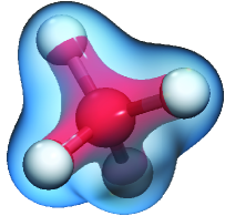
Figure 1: Methane molecule, CH₄. The blue and red isosurfaces denote low and high electronic density, respectively. Using our model, we have obtained for the angles between bonds, $109.47$ degrees, and a C-H bond distance of $106$ pm.

Kinetic theory, on the other hand, is the tool of choice for the study of transport phenomena in dilute media. It takes a mesoscopic point of view by defining the probability distribution function of finding a particle at a given position with a given momentum in the $6$-dimensional one-particle phase-space. This distribution function lives at the interface between the microscopic dynamics and the macroscopic description in terms of continuum fields representing average quantities over microscopic degrees of freedom Öttinger (2005).

In this Letter, we introduce a new approach to DFT, based on the kinetic theory, whereby the Kohn-Sham orbitals are regarded as density of quasi-particles, moving in an imaginary time, with the potential playing the role of a source or sink of quasi-particles. The dynamics of these quasi-particles is governed by a kinetic equation, which, upon Wick rotation to imaginary time, recovers the Kohn-Sham equations in the macroscopic limit of small mean free path. Using this kinetic approach, we compute the exchange and correlation energies of simple atoms and molecules, particularly the methane molecule (see Fig. 1). Excellent agreement with the literature is reported. Furthermore, due to the simple structure of the kinetic equation, it is argued that this approach might prove valuable also for developing an evolution equation for the total electronic density.

Let us begin by considering a many-body quantum system consisting of $N$ electrons. In the Kohn-Sham approach to DFT, this system is reduced to $N_{o}$ independent Schrödinger equations (Kohn-Sham equations), subject to a mean field potential that depends only on the total electronic density (Kohn theorem Hohenberg and Kohn (1964); Kohn and Sham (1965)), namely:

$$i\hbar\frac{\partial\psi_{i}}{\partial t}\quad=-\frac{\hbar^{2}}{2m}\nabla^{2}\psi_{i}+V\psi_{i},$$ (1)

where $V$ is the potential, $m$ the electron mass, and the index $i$ denotes the $i$-th electronic orbital. The total electronic density is approximated as $\rho\simeq\sum_{i}^{N_{o}}g_{i}|\psi_{i}|^{2}$, where $g_{i}$ is the occupation number (equal to $1$ for an open-shell and $2$ for a closed-shell) and $N_{o}$ denotes $N/2$ or $N/2+1$ for even and odd numbers of electrons, respectively. Since the eigenfunctions of the Hamiltonian form a complete basis in Hilbert space, any wave function $\psi^{\prime}$ that describes the state of a given orbital can be expanded onto this basis,

$$\psi^{\prime}(\vec{r},t)=\sum_{n}a_{n}\exp\left(i\frac{\epsilon_{n}t}{\hbar}\right)\phi_{n}(\vec{r})\quad,$$ (2)

where $a_{n}$ are projection coefficients defined via the inner product, $a_{n}=\langle\psi_{n}|\psi^{\prime}\rangle$, and $\phi_{n}(\vec{r})$ is the spatially dependent wave function, such that $\psi_{n}(\vec{r},t)=\phi_{n}(\vec{r})T_{n}(t)$. We have assumed that the potential does not depend explicitly on time. It is well-known that by using the Wick rotation, which consists in replacing $t\rightarrow i\tau$ (with $\tau$ an fictitious time), one obtains a diffusion equation with source term,

$$\frac{\partial\psi_{i}}{\partial\tau}=\frac{\hbar}{2m}\nabla^{2}\psi_{i}-\frac{V}{\hbar}\psi_{i}\quad.$$ (3)

Therefore, given an initial condition and using Eq. (2), we obtain $\psi_{i}(\vec{r},\tau)=\sum_{n}a_{n}\exp\left(-\epsilon_{n}\tau/\hbar\right)\phi_{n}$, where we see that for confined systems (negative energy eigenvalues), every term in the sum grows proportional to $\exp(|\epsilon_{i}|\tau/\hbar)$, while for unconfined systems (positive energy eigenvalues) each term decreases as $\exp(-|\epsilon_{i}|\tau/\hbar)$. In both cases, after some time, the only noticeable term in the sum will be the ground state, namely the one that grows fastest or decreases slowest, depending on the case. Therefore, the wave function $\psi_{0}$ will converge to $\psi_{i}\simeq a_{0}\exp(-\epsilon_{0}\tau/\hbar)\phi_{0}$, which, upon normalization, leads to the ground state. This time projection technique has been used to solve the Kohn-Sham system and obtain the ground state for different electronic configurations Chin et al. (2010); Auer et al. (2001).

However, since the diffusion equation can be derived from kinetic theory, it must be possible to recast the Kohn-Sham equations in the form of a kinetic equation in imaginary time. More precisely, the diffusion equation can be obtained from the Boltzmann equation,

$$\frac{\partial f}{\partial t}+\vec{v}\cdot\nabla f=\Omega(f)+S(\vec{r},\vec{v})\quad,$$ (4)

where $f=f(\vec{r},\vec{v},t)$ is a single distribution function defined in the phase space. Here, $S(\vec{r},\vec{v})$ represents a source term, and $\Omega$ is the collision operator. For simplicity, we approximate it with the Bhatnagar-Gross-Krook (BGK) relaxation operator Bhatnagar et al. (1954): $\Omega_{BGK}(f)=-(f-f^{eq})/\tau_{K}$, where $\tau_{K}$ is the kinetic relaxation time, and $f^{eq}$ the equilibrium distribution function, typically a local Maxwell distribution. Thus, by a Chapman-Enskog expansion Chapman and Cowling (1970), for small values of the Knudsen number $Kn$, defined as $Kn=\lambda/L$ $\lambda\propto\tau_{K}$ being the mean free path and $L$ the typical system size, we recover the diffusion equation for the density field $\rho$,

$$\frac{\partial\rho}{\partial t}=\tau_{K}{\cal D}\nabla^{2}\rho+{\cal S}\quad,$$ (5)

where $\rho=\int f\;d\vec{v}=\int f^{eq}\;d\vec{v}$, is the zeroth order moment of the distribution function, ${\cal S}=\int S\;d\vec{v}$ and ${\cal D}$ is defined according to the second order moment of the equilibrium distribution, ${\cal D}=\int f^{eq}\vec{v}^{2}\;d\vec{v}/\rho$. By comparing Eqs. (11) and (5), we observe that the Kohn-Sham equations emerge as the macroscopic limit of a distribution function of a gas of quasi-particles in phase space, with the identifications $\psi_{i}=\rho$, $(\hbar/2m)\psi_{i}=\tau_{K}{\cal D}\rho$, and $-V\psi_{i}/\hbar={\cal S}$.

Since we only require the zeroth, first, and second order moments of the equilibrium distribution (they are sufficient to recover the diffusion equation, and therefore the Kohn-Sham equations as well), we do not need to know the exact analytical expression of the equilibrium function (nor the intrinsic properties of the quasi-particles). Therefore, we can expand the distribution function onto an orthogonal basis of polynomials in velocity space up to second order. As a result, the distribution function, $f_{i}$, and the source term, $S_{i}$, related to each $i$-th orbital can be written as

$$f_{i}(\vec{r},\vec{v},t)=w(\vec{v})\sum_{n=0}^{\infty}a_{n,i}^{(n)}(\vec{r},t)H_{n}^{(n)}(\vec{v})\quad,$$ (6)

and $S_{i}=-(V/\hbar)f_{i}$, where $w(\vec{v})$ is the weight function, $a_{n,i}^{(n)}$ a tensor of order $n$, namely the projection of the distribution function upon the tensorial polynomial $H_{n}^{(n)}(\vec{v})$ of degree $n$,

$$a_{n,i}^{(n)}(\vec{r},t)=\int f_{i}(\vec{r},\vec{v},t)H_{n}^{(n)}(\vec{v})d^{3}v\quad.$$ (7)

As mentioned before, we could choose any kind of polynomials and weight functions that satisfy the first three order moment constraints. However, for simplicity we use the Hermite polynomials with the weight $w(\vec{v})=\exp(-\vec{v}^{2}/2\theta)/(2\pi\theta)^{3/2}$, $\theta$ being a normalized temperature. By using the first three normalized Hermite polynomials, $H_{0}=1$, $H_{1}^{k}=v^{k}/\sqrt{\theta}$, and $H_{2}^{kl}=(v^{k}v^{l}-\theta\delta^{kl})/\sqrt{2}\theta$, we can readily show that the equilibrium distribution function $f_{i}^{eq}$ for the $i$-th wave function becomes,

$$f_{i}^{eq}(\vec{r},\vec{v},t)=w(\vec{v})\psi_{i}(\vec{r})\left[1+\frac{{\cal D}-\theta}{2\theta^{2}}(\vec{v}^{2}-3\theta)\right]\quad,$$ (8)

where ${\cal D}=\hbar/(2m\tau_{K})$. Note that by taking $\theta={\cal D}$, implying that ${\cal D}$ behaves as the normalized temperature of the gas of quasi-particles, we obtain a simpler expression. However, we shall keep this general form for later applications, because, by increasing $\cal{D}$, i.e. the diffusivity $D={\cal D}\tau_{K}$, the particle dynamics can be accelerated and reach the equilibrium configuration faster.

Up to this point, there is no direct interaction between wave functions, and therefore they all reach the same ground state. In order to calculate excited states, hence impose the exclusion principle for fermions, we add an interaction potential, ${\cal V}_{i}$, to the Boltzmann equation for each wave function $\psi_{i}$. This yields

$$\frac{\partial f_{i}}{\partial t}+\vec{v}\cdot\nabla f_{i}=-\frac{1}{\tau_{K}}\left[\left(1+\frac{V\tau_{K}}{\hbar}\right)f_{i}-f_{i}^{eq}\right]-{\cal V}_{i}\quad,$$ (9)

with ${\cal V}_{i}=\sum_{j<i}\Lambda_{ij}f_{j}$, where $\Lambda_{ij}=\langle\psi_{i}|\psi_{j}\rangle/\langle\psi_{j}|\psi_{j}\rangle$. By introducing this potential, we dynamically and sequentially remove the contribution of excited levels $\psi_{j}$, with $j<i$, that do not belong to the respective orbital $i$. This is equivalent to a dynamic Gram-Schmidt orthogonalization procedure. Note that the interaction potential vanishes once the system reaches the ground state, since all orbitals are then orthogonal. The role of this potential is to generate local quasi-particles in order to satisfy the orthogonality conditions between the orbitals.

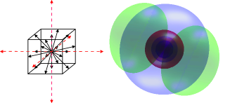
Figure 2: (Left) Lattice unit cell configuration D3Q25 ( $25$ discrete velocities in $3$ dimensions). The solid arrows denote the vectors pointing to the first two neighbors, and the dashed lines, the ones with length $|\vec{v}_{j}|=3$. (Right) Electronic orbital density of the carbon atom, the red, blue, and green isosurfaces denote the first ($1s$), second ($2s$), and third ($2p$) orbitals at $\psi^{2}_{0,1,2}=10^{-5}$ au, respectively.

To summarize, we have converted the system of $N_{o}$ original Kohn-Sham equations into $N_{o}$ kinetic equations. In this approach, we need to solve Eq. (9), using Eq. (8). Note that Eq. (9) has no second order spatial derivatives and therefore space and time go on the same footing. This offers a number of computational advantages, as we shall detail shortly.

The energy of each orbital can be calculated through the relation, $\epsilon_{i}=-(\hbar/2)\partial\log(\langle\psi_{i}|\psi_{i}\rangle)/\partial t$.

In order to check the validity of our approach, we develop a numerical scheme and implement different simulations for simple atoms and molecules. As it stands, Eq. (9) looks computationally over-demanding, since it lives in a six-dimensional phase space. However, for the purpose of solving hydrodynamic problems, it is known that velocity space can be constrained to a handful of properly chosen discrete velocities $\vec{v}=\vec{v}_{j}$, where $j$ runs over a small neighborhood of any given lattice site. This strategy has spawned a powerful technique, known as Lattice Boltzmann method, which has proven very successful for the simulation of a broad variety of complex flows Benzi et al. (1992); Chen et al. (1992); Succi (2001); Mendoza and Muñoz (2010); Bernaschi et al. (2009). In the present work we employ the $25$ discrete velocities shown in Fig. 2. The result is the following set of Lattice Kinetic Kohn-Sham equations (LKKS):

$$f_{ij}(\vec{r} +\vec{v}_{j}\delta t,t+\delta t)-f_{ij}(\vec{r},t)=$$ (10)

$$-\frac{\delta t}{\tau_{K}}\biggl{[}\biggl{(}1+\frac{V\tau_{K}}{\hbar}\biggr{)}f_{ij}(\vec{r},t)-f_{ij}^{eq}(\vec{r},t)\biggr{]}-{\cal V}_{ij}\quad,$$

where ${\cal V}_{ij}=\sum_{k<i}\Lambda_{ik}f_{kj}$. Further details on the discretization and the values of the numerical parameters for the following simulations are presented in the Supplementary Material sup .

We first calculate the exchange and correlation energies for four different atoms, H, Be, B, and C. For this purpose, we have used a lattice size of $64^{3}$ cells. The measured values for the exchange and correlation energies are given in Table 1, together with the computational time and number of iterations taken by the discretized model. In Fig. 2, we show the orbitals obtained for the carbon atom, finding very good qualitative results.

Atom	${\cal V}_{x}$	Exp. ${\cal V}_{x}$	${\cal V}_{c}$	Exp. ${\cal V}_{c}$	Time	Iterations
H	$-0.310$	$-0.310$	$0$	$0$	$3$ min	$640$
Be	$-2.651$	$-2.658$	$-0.096$	$-0.095$	$17$ min	$3035$
B	$-3.742$	$-3.728$	$-0.127$	$-0.128$	$21$ min	$3009$
C	$-5.084$	$-5.032$	$-0.173$	$-0.161$	$18$ min	$2968$

Table 1: Exchange-Correlation energies for H, Be, B, and C. Computational time and the number of iterations performed by the model to reach the ground state are also shown. The expected values of exchange, ${\cal V}_{x}$, and correlation, ${\cal V}_{c}$, energies are taken from Refs. Becke (1988); Lee et al. (1988).

The differences between the obtained and expected exchange and correlation energies are of the order of $1\%$ except for the case of the correlation energy of the carbon atom. The large error for this case is due to the larger spatial extension of $p$ orbital (see Fig. 2) which makes it sensitive to the boundary conditions. The computational time of these simulations is measured when the energy of the orbitals presents changes of less than $10^{-5}\%$ between two subsequent steps.

Our kinetic equations can also be solved in dynamic fashion, i.e. by evolving the Kohn-Sham orbitals concurrently with the ionic motion (Concurrent Dynamics, CD for short). Although a rigorous theoretical support for such a procedure remains to be developed, we performed a study of how small the time step in the CD implementation of our algorithm should be, in order for the system to remain sufficiently close to the Born-Oppenhemier (BO) surface. To this purpose, we compare both versions of our kinetic scheme, BO and CD, against each other. For this case, we excite the H₂ molecule and let it vibrate in its first mode. We have used a lattice size of $24^{3}$ cells. Note that by choosing the same time step, $\delta t=0.00228$ fs, (see Fig. 3), CD does not conserve the energy of the system, and the amplitude of the oscillations decays in time. However, by choosing an eight times smaller time step, the CD shows excellent agreement with BO, still performing three times faster than BO (CD took $20$ minutes and BO $73$ minutes on the same machine). The oscillation frequency of the vibrational mode obtained by the simulation is $4789$ cm^-1, which presents an error of $15\%$ in comparison with the experimental value of $4161$ cm^-1 Stoicheff (1957). This discrepancy is not inherent to our approach, but is rather due to discretization errors. Improvements of the numerical integration of the kinetic equations will be a subject of future work.

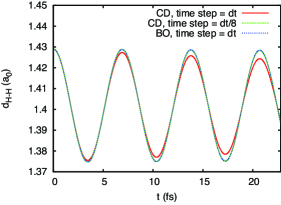
Figure 3: Vibrational mode of the diatomic molecule H₂. Here BO and CD denote Born-Oppenheimer and Concurrent Dynamics, respectively. The time step for this simulation is $\delta t=0.00228$ fs.

Finally, we build the methane molecule from scratch, by using the bare Coulomb potential. For this simulation, we use a lattice size of $84^{3}$ cells, and place the carbon atom in the center of the simulation zone. The hydrogen atoms are located randomly in space, and we let the system evolve to the ground configuration. After a few hours, we achieved the configuration shown in Fig. 1. Note that the angles are reproduced precisely, $109.47$ degrees, but the bond distance of $106$ pm is slightly shorter than the experimental value of $\sim 108.5$ pm Bowen-Jenkins et al. (1988). This bond distance discrepancy is due to finite-size boundary effects, which compress the molecule. This statement is supported by further simulations with larger system sizes. The fact that we can reproduce the angles exactly with the bare Coulomb potential, is encouraging, since the use of pseudo-potentials requires orbital dependent parameters, which may significantly increase the complexity of the simulation.

Summarizing, we have introduced a new approach to DFT based on Boltzmann’s kinetic theory. We have shown that the Kohn-Sham equations can be regarded as a macroscopic limit of a first-order Boltzmann kinetic equation. In the kinetic Kohn-Sham equations, we assume that the ground state of a quantum system can be regarded as a gas of quasi-particles, which are generated or destroyed by the potential, the different wave functions interacting with each other in such a way as to match the orthogonality constraints. This opens a new perspective in the interpretation of multi-electron quantum systems.

The kinetic approach offers a number of computational advantages. First, since diffusion emerges from the underlying first-order propagation-relaxation microscopic dynamics, space and time always appear on the same footing (no second order spatial derivatives). This permits to advance the system in time with a time-step scaling only linearly with the mesh resolution, rather than quadratically. Second, since the information always travels along straight lines, defined by the discrete velocities $\vec{v}_{j}$, the streaming is computationally exact (zero round-off error). Third, owing to its excellent amenability to parallel computing, the present lattice kinetic formulation is expected to prove particularly valuable for large-scale simulations.

The lattice kinetic approach has shown excellent performance and accuracy. It can calculate satisfactorily molecular structures by using the bare Coulomb potential, obtaining the right geometric configuration, as it is the case for the methane molecule, without dealing with complicated orbital dependent pseudo-potentials. However, for large molecular structures, the inclusion of pseudo-potentials might well become necessary. We have also performed computational benchmarks and compared the performance with Car-Parrinello molecular dynamics Car and Parrinello (1985) (CPMD), finding satisfactory results for the computational time to ground state, at least for simple molecules. The details of these benchmarks are provided in the Supplementary Material sup .

Finally, the present kinetic approach appears well positioned to solve the evolution equation for the total electronic density, by implementing the analogous of the Chapman-Enskog expansion for classical fluids. This, together with improvements of the discretization, such as local grid refinement, should permit to extend the present lattice kinetic approach to many challenging ab initio calculations, possibly including those currently handled by time-dependent density functional theory Marques and Gross (2004).

Appendix A Supplementary Material

Appendix B Theoretical Background

The aim of this supplementary material is to show the discretized form of the kinetic equations, which in the macroscopic limit reproduce the Kohn-Sham equations with imaginary time,

$$\frac{\partial\psi_{i}}{\partial t}=\frac{\hbar}{2m}\nabla^{2}\psi_{i}-\frac{V}{\hbar}\psi_{i}\quad.$$ (11)

The potential energy of the system, $V$, according to the theorem of Kohn, should only depend on the total electronic density $\rho$, and, by using mean field approximations, contains four parts $V=V_{ext}+V_{ee}+V_{xc}$, where $V_{ext}$ is the external potential due to ions and/or external interactions, $V_{ee}$ is the interaction between electrons, and $V_{xc}$ is the exchange-correlation interaction. For a multi-electronic system interacting with $N_{i}$ ions, we can write $V_{ext}$ as, $V_{ext}(\vec{r})=-(1/4\pi\varepsilon_{0})\sum_{i}^{N_{i}}(Z_{i}e^{2})/(|\vec{r}-\vec{R}_{i}|)$, where $Z_{i}$ is the atomic number of the $i$-th ion, $e$ is the charge of the electron, and $R_{i}$ the position of each ion. The electron-electron interaction, $V_{ee}=e\Phi$, is obtained by solving the Poisson equation for the electric potential $\Phi$, $\nabla^{2}\Phi=e\rho/\varepsilon_{0}$.

For the exchange-correlation potential $V_{xc}$, we use the functional derivative of the exchange-correlation energy ${\cal V}_{xc}=\delta{\cal V}_{xc}/\delta\rho$. Here we use the approach by Becke Becke (1988) and Lee et al. Lee et al. (1988). The Laplacians and gradients of the total density needed to calculated the exchange and correlation potentials, are computed by using an elegant fourth-order method recently proposed in Ref. Thampi et al. (2013).

The ions move following classical molecular dynamics where the Hellman-Feynman forces due to the electron density are introduced via the electric potential $\Phi$, dictated by the spatial distribution of the electronic charge. In our case, the Hamiltonian of the $j$-th ion is given by ${\cal H}_{j}=\vec{P}_{j}^{2}/2M_{j}+Z_{j}e\Phi+\sum_{i\neq j}^{N_{i}}Z_{i}Z_{j}e^{2}/(4\pi\varepsilon_{0}|\vec{R_{j}}-\vec{R}_{i}|)$, where $Z_{i}$ is the atomic number, $M_{j}$ the ion mass and $\vec{P}_{j}$ the ion momentum. Due to the Born-Oppenheimer approximation, for each movement of the ions, the electronic density must be updated at the ground state. Here we will not consider photon or phonon emissions, i.e. the electrons adapt instantaneously to the ground state after the motion of the ions. Furthermore, for the purpose of this work, we will only take into account the electron-ion and ion-ion electrostatic interations, and therefore consider small time steps in order to conserve the total energy of the system Meng and Kaxiras (2008). However, to be precise, one would need to use instead of just the electrostatic interaction, the total Hamiltonian of the electrons. Extensions in this direction will be subject of future research.

Appendix C Lattice Kinetic Description

Our model is based on the lattice Boltzmann method. Therefore, we define the distribution function $f_{ij}(\vec{r},t)$ that describes the dynamics of the orbital $\psi_{i}$ and is associated with the velocity vector $\vec{v}_{j}$. For this purpose, we will use a special case of the Boltzmann equation ($\tau_{K}=\delta t=1$) that lets the system evolve using just the equilibrium function,

$$f_{ij}(\vec{r}+\vec{v}_{j},t+1)=w_{j}\psi_{i}(\vec{r},t)\left[1+\frac{\theta-{\cal D}}{2\theta^{2}}\left(3\theta-\vec{v}_{j}^{2}\right)\right]\quad,$$ (12)

where $w_{i}$ are discrete weights and $\theta$ is the lattice temperature, which are defined depending on the cell configuration, and ${\cal D}=\hbar/m$ (note that for the analytical equilibrium distribution in the main text, ${\cal D}=\hbar/2m$, here the factor $1/2$ will appear as a consequence of the discretization). Standard LB practice shows that in the continuum limit, the above equation converges to a diffusion-reaction equation (such is the Kohn-Sham with imaginary time, Eq. (11)) for the “density” $\psi_{i}(\vec{r},t)=\sum_{j}f_{ij}(\vec{r},t)$. This is more memory intensive than a standard finite-difference scheme, but offers significant advantages in return. First, since diffusion is emergent from the relaxation to local equilibrium, i.e. the rhs of (12), no Laplacian is required, hence the time-step scales only linearly with the mesh size, rather than quadratically. Second, since the local equilibrium at the rhs is integrally shifted to the neighbor locations $\vec{r}+\vec{v}_{j}$, the spatial transport component of the algorithm is virtually exact, i.e. zero round-off error. Third, the local equilibrium conserves the local density to machine roundoff. All of the above configures LB as a very fast, second-order accurate scheme for diffusion-reaction equation. Second order accuracy might appear poor as compared to, say, spectral methods, but the three aforementioned properties make the coefficients of second order errors so small that LB has indeed been shown to provide similar accuracy as spectral methods for, say, turbulence simulations on grids of the order $O(10^{3})$.

The functions $\psi_{j}$ contain a forcing term in order to satisfy the second term in the rhs of Eq. (11) and the orthogonality conditions between electronic orbitals. Thus, we can write the wave function as,

$$\psi_{j}=\left(\psi^{\prime}_{j}-V_{ar,\;j}\right)/(1+V)\quad.$$ (13)

Note that the second term is the interaction potential $V_{ar,\;j}=\sum_{k<j}\psi^{\prime}_{k}\langle\psi^{\prime}_{j}|\psi^{\prime}_{k}\rangle/\langle\psi^{\prime}_{k}|\psi^{\prime}_{k}\rangle$ that ensures the orthogonality condition of the wave functions $\psi_{j}$ and it vanishes once the system reaches the ground state. This potential is kind of a time-dependent Gram-Schmidt procedure. The auxiliary fields $\psi^{\prime}_{j}$ are obtained from the distribution functions $f_{ij}$, $\psi^{\prime}_{j}=\sum_{i}^{\cal N}f_{ij}$, where $\cal N$ is the number of velocity vectors.

Increasing the lattice temperature, $\theta$, implies to increase the number of velocity vectors, allowing a faster convergence but also introducing errors of higher order derivatives. After a systematic study of different configuration for the velocity vectors, and following the procedure in Ref. Chikatamarla and Karlin (2009), we have found a new cell that gives the best performance and accuracy, D3Q25, which can be seen in Fig. 2 in the main text. The weights $w_{i}$ and velocity vectors, $\vec{v}_{i}$ can be derived from the equations in Ref. Chikatamarla and Karlin (2009), for the case of $\theta=1-\sqrt{2/5}$.

Thus, at each time step, we know the wave functions $\psi_{j}$, and can calculate the electronic density using $\rho=\sum_{j}^{N_{o}}g_{i}|\psi_{j}|^{2}$. For the computation of the exchange and correlation potentials, we cannot use $\rho$, since it depends itself of the potentials via Eq. (13), leading to highly complicated system of non-linear algebraic equations. Therefore, as a reasonable guess, we take the density calculated with $\psi^{\prime}_{j}$, $\rho^{\prime}=\sum_{j}^{N_{o}}g_{i}|\psi^{\prime}_{j}|^{2}$.

For the Poisson equation, we implement an additional diffusion equation using $\varphi_{i}$ as the distribution functions that model the electric potential $\Phi$. For this distribution, we have as evolution equation,

$$\varphi_{i}(\vec{r}+\vec{v}_{i},t+1)=w_{i}\Phi\left[1+\frac{\theta-\nu}{2\theta^{2}}\left(3\theta-\vec{v}_{i}^{2}\right)\right]\quad,$$ (14)

where $\nu$ is a given diffusion parameter that tunes how fast the potential $\Phi$ converges to the solution of the Poisson equation. Due to the presence of charge density, we have to modify the potential with the expression, $\Phi=\sum_{i}^{\cal N}\varphi_{i}+\rho\nu/2\varepsilon_{0}$.

The energy level of each orbital can be calculated as, $\epsilon_{j}=(\hbar/2)\log\left(\langle\psi^{\prime}_{j}|\psi^{\prime}_{j}\rangle|_{t}/\langle\psi^{\prime}_{j}|\psi^{\prime}_{j}\rangle|_{t+1}\right)$, which converges to a constant value once the system reaches the ground state. For the dynamics of the ions we use the Verlet method. In order to have an accurate value of the forcing term, we use a cubic interpolation to calculate the gradients of the potentials at the location of each ion.

Appendix D Details of the Different Simulations

In order to validate our model, we have performed several simulations, whose details are presented here. First, we show the details of the simulation for calculating the exchange and correlation energies for four different atoms, H, Be, B, and C. Next, we implement a comparison with Car-Parrinello molecular dynamics Car and Parrinello (1985) (CPMD) for the case of the hydrogen molecule, and finally, we present the numerical details of the simulation of the first vibrational mode of the hydrogen molecule and the respective details of the calculation of the geometry of the methane molecule.

D.1 Exchange and Correlation energies for several atoms

In all cases, we take a lattice size of $64^{3}$ cells, and fix the Bohr radius to $6$, $9$, $10$, and $12$ cells, for H, Be, B, and C, respectively. We have also set ${\cal D}=\nu=0.85$. This implies that we are fixing the relation between the Planck constant and the electronic mass via the parameter ${\cal D}$. The consequences of this assumption are only numerical, since we can always make a conversion of units where the natural constants, e.g. speed of light, Boltzmann constant, Plank constant, electronic charge and mass, etc., have arbitrary numerical values.

D.2 Comparison with CPMD

Although a fair comparison with CPMD is not possible because it uses pseudo-potentials, we will perform simulations for small molecules where the valence electrons are also core electrons, i.e. hydrogen and helium molecules. In order to model the hydrogen molecule, we consider two hydrogen atoms separated by a distance $d=1.401a_{0}$ (equilibrium configuration), with $a_{0}$ the Bohr radius, and we let the system optimize the wave function of the ground state, using both, CPMD and our model. Since our model starts with a constant wave function, we will use for CPMD, as initial pseudopotential and wave function, LDA exchange-correlation term, adjusted in the CPMD input file to optimize the wave function taking into account the exchange-correlation model proposed by Becke-Lee-Yang-Parr (BLYP) Becke (1988); Lee et al. (1988). The reason for this choice is to make the comparison between both methods as fair as possible. In our model, we have set ${\cal D}=\nu=0.85$.

	$20^{3}$	$24^{3}$	$32^{3}$	$70$	$140$	$280$
${\cal V}_{xc}$	$-0.695$	$-0.695$	$-0.695$	$-0.692$	$-0.694$	$-0.694$
$\%$ Error	$\ll 0.1$	$\ll 0.1$	$\ll 0.1$	$0.4$	$0.1$	$0.1$
Time (s)	$3$	$9$	$38$	$13$	$32$	$87$
Iterations	$343$	$488$	$850$	$10$	$10$	$10$

Table 2: Time consumption to optimize the wave function of the ground state for the H₂ molecule using our model and CPMD package. The errors are computed with the expected value ${\cal V}_{xc}=-0.695$ reported in Ref. Polo et al. (2009). The first three columns correspond to LB (for lattice sizes of $20^{3}$, $24^{3}$, and $32^{3}$), and the last three to CPMD (cutoff of $70$, $140$, and $280$) calculations.

In Table 2, we show the results of the time consumption for our model for different system sizes. For $20^{3}$, $24^{3}$ and $32^{3}$, where we have chosen $a_{0}=2.5,3.0$, and $3.6$, respectively. We have used different lattice sizes to check convergence and boundary effects. The lattice $20^{3}$ is quite small and nevertheless can optimize properly the wave function. This is one of the main advantages of our model, the possibility to obtain reasonable accuracy by using few lattice sites. Also, in Table 2, we can see the performance of CPMD for the same configuration. Here, we have used different cutoffs for the plane wave expansion. Note that the times are of the same order as the ones of LB. In both cases, the tolerance of error has been adjusted to $10^{-5}\%$.

Let us now take two atoms of hydrogen and locate them at twice their equilibrium distance, $d=2.8a_{0}$, and let the system optimize the position of the atoms until reaching the ground state. For our model, we use again ${\cal D}=\nu=0.85$, and we have chosen a time step of $\delta t=200$ ($0.16$ ps), and the tolerance of both, the electronic density and ion dynamics, of $10^{-5}\%$. The lattice size is $20^{3}$ cells.

Model	LB ($20^{3}$)	CPMD (70)	CPMD (140)
Time (s)	9	139	324
Final $d$ ($a_{0}$)	$1.402$	$1.414$	$1.409$
Error $\%$	$0.07$	$0.9$	$0.6$

Table 3: Time consumption to optimize the geometry to the ground states using both models, LB and CPMD. For the case of CPMD, the the number inside the parenthesis denotes the cutoff. The errors are calculated with the equilibrium distance of $d=1.401a_{0}$.

In the case of CPMD, we have implemented several simulations for different cutoffs and using for the spatial optimization a tolerance of $10^{-3}\%$ and for the wave function optimization $10^{-5}\%$. In Table 3 are shown the results of the time consumption for both methods and also the final distance between the atoms. For this test, CPMD has shown to be almost one order of magnitude slower than our model, and even without achieving a very good accuracy for the equilibrium configuration which is around $1.401a_{0}$. These results show that our model can be very competitive for ab initio simulations of the ground state. All simulations for the comparison with CPMD have been run on a single core of an Intel Xeon E 5430 processor at 2.66 GHz.

D.3 Concurrence and Born-Oppenheimer Dynamics

The numerical parameters are the same as in the previous simulations in Sec. D.2.

D.4 Methane molecule

For building the methane molecule from scratch, we use a lattice size of $84^{3}$ cells, and we place the carbon atom in the center of the simulation zone. The hydrogen atoms are located randomly in space, and we let the system evolve towards the ground configuration. We have chosen the same parameters as before and a Bohr radius of $11$ cells. After $8$ hours, we have achieved the final configuration.

References

- Gross and Dreizler (1995) E. Gross and R. Dreizler, Density Functional Theory, NATO ASI Series: Physics (Springer, 1995).
- Hohenberg and Kohn (1964) P. Hohenberg and W. Kohn, Phys. Rev. 136, B864 (1964).
- Kohn and Sham (1965) W. Kohn and L. J. Sham, Phys. Rev. 140, A1133 (1965).
- Becke (1988) A. D. Becke, Phys. Rev. A 38, 3098 (1988).
- Lee et al. (1988) C. Lee, W. Yang, and R. G. Parr, Phys. Rev. B 37, 785 (1988).
- Meng and Kaxiras (2008) S. Meng and E. Kaxiras, The Journal of Chemical Physics 129, 054110 (2008).
- Polo et al. (2009) V. Polo, E. Kraka, and D. Cremer, Molecular Physics: An International Journal at the Interface Between Chemistry and Physics 100, 1771 (2009).
- Kühne et al. (2009) T. D. Kühne, M. Krack, and M. Parrinello, Journal of Chemical Theory and Computation 5, 235 (2009).
- Remler and Madden (1990) D. K. Remler and P. A. Madden, Molecular Physics 70, 921 (1990).
- Hutter (2012) J. Hutter, Wiley Interdisciplinary Reviews: Computational Molecular Science 2, 604 (2012).
- Kühne et al. (2007) T. D. Kühne, M. Krack, F. R. Mohamed, and M. Parrinello, Phys. Rev. Lett. 98, 066401 (2007).
- Car and Parrinello (1985) R. Car and M. Parrinello, Phys. Rev. Lett. 55, 2471 (1985).
- Öttinger (2005) H. Öttinger, Beyond Equilibrium Thermodynamics (Wiley, 2005).
- Chin et al. (2010) S. A. Chin, S. Janecek, E. Krotscheck, and M. Liebrecht, International Journal of Modern Physics B 24, 4923 (2010).
- Auer et al. (2001) J. Auer, E. Krotscheck, and S. A. Chin, The Journal of Chemical Physics 115, 6841 (2001).
- Bhatnagar et al. (1954) P. L. Bhatnagar, E. P. Gross, and M. Krook, Phys. Rev. 94, 511 (1954).
- Chapman and Cowling (1970) S. Chapman and T. Cowling, The Mathematical Theory of Non-uniform Gases: An Account of the Kinetic Theory of Viscosity, Thermal Conduction and Diffusion in Gases, Cambridge Mathematical Library (Cambridge University Press, 1970).
- Benzi et al. (1992) R. Benzi, S. Succi, and M. Vergassola, Physics Reports 222, 145 (1992).
- Chen et al. (1992) H. Chen, S. Chen, and W. Matthaeus, Physical Review A 45, 5339 (1992).
- Succi (2001) S. Succi, The lattice Boltzmann equation for Fluid Dynamics and Beyond (Oxford University Press, New York, 2001).
- Mendoza and Muñoz (2010) M. Mendoza and J. D. Muñoz, Phys. Rev. E 82, 056708 (2010).
- Bernaschi et al. (2009) M. Bernaschi, S. Melchionna, S. Succi, M. Fyta, E. Kaxiras, and J. K. Sircar, Computer Physics Communications 180, 1495 (2009).
- (23) See Supplementary Material at.
- Stoicheff (1957) B. P. Stoicheff, Canadian Journal of Physics 35, 730 (1957).
- Bowen-Jenkins et al. (1988) P. Bowen-Jenkins, L. G. M. Pettersson, P. Siegbahn, J. Almlof, and P. R. Taylor, The Journal of Chemical Physics 88, 6977 (1988).
- Marques and Gross (2004) M. Marques and E. Gross, Annual Review of Physical Chemistry 55, 427 (2004), pMID: 15117259.
- Thampi et al. (2013) S. P. Thampi, S. Ansumali, R. Adhikari, and S. Succi, Journal of Computational Physics 234, 1 (2013).
- Chikatamarla and Karlin (2009) S. S. Chikatamarla and I. V. Karlin, Phys. Rev. E 79, 046701 (2009).