Beyond Physical Connections: Tree Models in Human Pose Estimation

Abstract

Simple tree models for articulated objects prevails in the last decade. However, it is also believed that these simple tree models are not capable of capturing large variations in many scenarios, such as human pose estimation. This paper attempts to address three questions: 1) are simple tree models sufficient? more specifically, 2) how to use tree models effectively in human pose estimation? and 3) how shall we use combined parts together with single parts efficiently?

Assuming we have a set of single parts and combined parts, and the goal is to estimate a joint distribution of their locations. We surprisingly find that no latent variables are introduced in the Leeds Sport Dataset (LSP) during learning latent trees for deformable model, which aims at approximating the joint distributions of body part locations using minimal tree structure. This suggests one can straightforwardly use a mixed representation of single and combined parts to approximate their joint distribution in a simple tree model. As such, one only needs to build Visual Categories of the combined parts, and then perform inference on the learned latent tree. Our method outperformed the state of the art on the LSP, both in the scenarios when the training images are from the same dataset and from the PARSE dataset. Experiments on animal images from the VOC challenge further support our findings.

1 Introduction

Tree models are very efficient in a number of computer vision tasks such as human pose estimation and other articulated body modeling. These models prevail because they are simple and exact inference is available. Also because of these unique advantages, it is not uncommon to speculate that tree models may not effectively handle computer vision problems in real world applications.

As a consequence, latent variables [1] and loopy graphical models [2] were proposed in the past few years for human pose estimation as the remedy of the problems caused by those “oversimplified” tree models. All these methods have their advantages both in theory and practice, and performance improvements are significant. Particularly, it is believed that loopy graphical models are necessary when combined parts (or “poselet”) are used to handle large variance in appearance. However, no theoretical analysis shows 1) how to combine parts in component-based learning for computer vision, and 2) which model is optimal.

In this paper, we argue that the simple tree model is still a very powerful representation, and combined parts and single parts can be used together without sacrificing the benefits brought by exact inference. We further address how to use it optimally in human pose estimation.

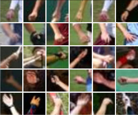
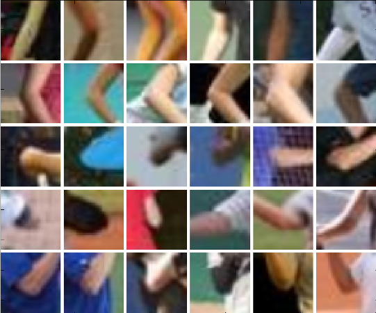
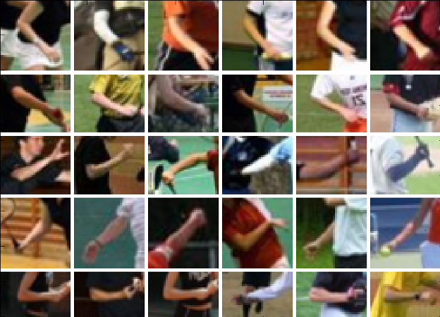
(a) Hand	(b) Elbow	(c) Upper arm	(d) Lower arm	(e) Lower leg

Figure 1: Examples of types in the LSP dataset. The types for single parts a) and b) are defined by their relative positions to their neighbors. For combined parts c)-e), the types are defined by their visual categories. Each row represents one type of a part.

All the questions about tree models arise when we start to use the skeleton as the tree structure. While this “mapping” is apparent, no evidence claims it is optimal. Further, this limits our choices of representation, as well as complicates the graphical model when combined parts are introduced.

Our goal is to learn a tree model directly from observed variables. These observations can be body part locations, as used in many recent pose estimation papers. At the same time, this allows us to introduce more variables such as combined parts, as long as they can be observed and the state space is the same as that of single body parts.

A significant advantage of our framework is that single joints and body limbs are considered in the same level in inference. Recent advancements in learning graphical models enable us to learn latent trees from these observations. The latent tree models suggest that we could approximate the joint distribution of the observations by a tree model, and latent variables are introduced only when necessary.

We start our journey by exploring the property of the latent tree models. It is not surprising that the resulting latent tree has a similar structure to human skeleton. What really surprising is that there was no hidden variable added when we applied it to the Leeds Sport dataset (LSP) [3]. This human pose estimation dataset is challenging both in the pose variations and its size. Therefore, this implies we can directly use a tree model with mixed types of variables for human pose estimation to approximate the true distribution.

This exciting claim cannot be achieved without the appearance model. While the state space of these observations is the same (i.e., spatial location), their appearance models vary. We used “types”, a concept in recent papers, to capture the appearance clustering [4, 1].

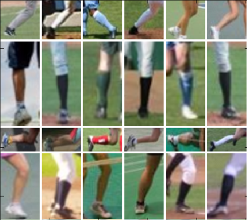
The types were proposed to define the possible configurations between adjacent nodes in graphical model [4]. We follow this guideline, but redefine the type being its Visual Category if a node represents a combined part (Fig. 1). The concept of visual category is no stranger to computer vision and pose estimation. Unlike other state of the arts in human pose estimation that use only a small number of categories, we find that a larger number of visual categories facilitates pose estimation. This also makes our framework unlimited to the physical connections [5], and flexible to other articulated objects estimation in computer vision.

The inference of our model is very efficient due to the tree structure, and results suggest that our method outperforms state of the art on the LSP dataset. We further tested our model in a cross-dataset experiment, where we used PARSE [6] dataset for training and LSP for testing. Our performance does not decrease in this challenging test. Finally, we verified our hypothesis by testing on a subset of animal images in the VOC dataset [7].

Our contributions include:

• We propose to learn tree models for articulated pose estimation problems.

• Our method effectively exploits the interactions between combined parts and single parts.

• Our method outperforms the state of the art in human and animal pose estimation.

2 Related work

Human pose estimation

Human pose estimation has been formulated as a part based inference problem. Appearance model and deformable model that describe relations between parts were proposed in the past decade.

Rich appearance models were adopted extensively in estimating human poses. Histogram of Oriented Gradient (HOG) [8] were frequently used as the features for the appearance model of body parts. Bourdev et al. [9] proposed the idea of poselets as the building blocks for human recognition, which refers to combined parts that are distinctive in training images.

One successful example of deformable models is the Pictorial Structure Model (PSM) [5]. Pairwise terms in human pose estimation are represented as relative distance between two parts. Such definition allows efficient distance transform method to be used in message passing process. Yang et al. [4] proposed a flexible mixtures-of-parts model for articulated pose estimation. Instead of modeling both location and orientation of each body part as rigid part, they used the model that only contains non-oriented parts with co-occurrence constraints.

It is widely hypothesized that graphical models that go beyond pairwise links lead to better performance in pose estimation. Loopy graph model may give more precise results, but it takes more efforts to solve [2]. Several new approaches also use latent nodes [1] or hierarchical graph models [10].

In this paper, we examine the above concepts, and suggest that these important components in articulated body detection and pose estimation can be integrated in an efficient framework. Therefore, we exploit a newly developed technique in learning latent tree models.

Latent tree models

The latent tree models [11] aim at finding tree approximations of joint distribution of observable variables. Using trees to approximate joint distribution has been dated to the early days of machine learning. In Chow-Liu tree [12] all nodes in the latent tree must be observable. Recently, Choi et al. [11] proposed two algorithms on learning latent trees. Their methods automatically build tree structures from observations, using information distances as the guideline of merging nodes and introducing latent variables.

This theoretical approach is very useful for human pose estimation, because we can learn a structure directly from our observations without making many assumptions of the physical constraints, while the performance is still guaranteed in terms of approximating the joint distribution.

3 Latent tree models for pose estimation

First, we provide a brief introduction to the latent tree models, and show the results on modeling the body joints in the LSP using latent tree models. We then present the learning of visual category for combined parts, which is necessary in our model for reducing complexity. Finally, we present our tree based inference model.

Figure 2: Latent tree models learned from the LSP dataset. From left to right, the results for CLGrouping tree, CL-Neighbor Joining [11] using single parts, respectively, and CLGrouping on single and combined parts together. The circles denote single parts, and the squares denote combined parts.

3.1 Brief introduction to latent tree models

The goal of latent tree model is to recover a tree-structured graphical model that best approximates the distributions of a set of observations. Recursive Grouping and CLGrouping were proposed in [11] to create latent tree models without any redundant hidden nodes. The authors demonstrated their methods on real-world datasets by modeling the dependency structure of monthly stock returns in the S&P index and of the words in the 20 newsgroups dataset. Please note that in the resulting models, the observed variables can be both leaf nodes and non-leaf nodes.

We briefly describe recursive grouping in this section due to its simplicity. CLGrouping is its extension that can build up latent tree structures for large diameter graphs more efficiently with a pre-processing step.

In this grouping method, the latent tree were built recursively by identifying sibling groups using information distances. Given two observed random variables $X_{i}$ and $X_{j}$, the correlation coefficient is defined as

$$\rho_{ij}=\frac{\text{Cov}(X_{i},X_{j})}{\sqrt{\text{Var}(X_{i})\text{Var}(X_{j})}}$$ (1)

and the information distance is defined as

$$d_{ij}=-\text{log}(\rho_{ij})$$ (2)

Then, the recursive grouping method build up the latent tree by testing relationships among each triplet $i,j,k\in V$. Define $\Phi_{ijk}\triangleq d_{jk}-d_{ik}$, take one of the two actions below:

• If $\Phi_{ijk}=d_{ij},$ $j$ is set to be the parent of $i$.

• If $-d_{ij}\leq\Phi_{ijk}=\Phi_{ijk^{\prime}}\leq d_{ik}$ for all $k$ and $k^{\prime}\in V\backslash\{i,j\}$, add a hidden node as the parent of $i$ and $j$.

In this way, a latent tree is recursively built. Please refer to [11] for details.

3.2 Latent trees for human pose

Our goals is to use single parts and combined parts in the inference model. Given image $I$, we define $P$ parts as $p_{i}=(loc_{i},t_{i}),i\in[1,...,P]$, where $loc_{i}$ is the part location in images, $t_{i}$ is either visual category label for combined parts (Sec 3.3), or represents different morphologies of parts for single parts as suggested in [4]. Two possible part combinations in our case are:

• Connected parts: A combined part may have physical connection in human body. This is a natural choice for many problems, because connected parts (e.g., upper arm and lower arm) may have higher correlations in general.

• Physically separated parts: The combined parts can be used for encoding semantic relations among single parts. This can be totally data driven. For instance, in many applications arm poses are symmetric. Therefore, one may combine these two physically separated parts as one element.

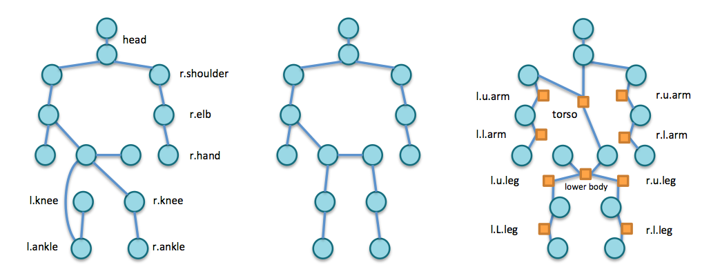
In our following experiment, we defined 14 single parts and 10 combined parts (Fig. 2). We used their spatial correlation in the image space as the mutual information, and Fig. 2 shows the results by three different algorithms. We tested two scenarios in our experiment:

• Single parts only: In this experiment, we used only single parts for the latent tree models. Fig. 2 shows two results using CLGrouping tree and CL-Neighbor Joining [11]. It is not very surprising that the structure is similar to human body, but please note that there is no latent node introduced by CLGrouping method in such a complicated and challenging dataset. Because no redundant latent nodes is used in latent tree model, this means the joint distributions of all body joints can be approximated by a simple tree structure.

• Single+combined parts: Due to the limitation of appearance model, it is more effective to use combined parts in appearance model for detecting parts. Therefore, introducing combined parts is a solution in many algorithms. We used both single and combined parts in the latent tree models (Fig. 2). Again, the output has no latent variables. This means we can approximate the joint distribution by combined parts and single parts in a tree structure.

This finding makes our latent tree model different from [1], because all our nodes are observable. Also, this is different from [2], because our structure is a tree.

.

Figure 3: Examples of visual category. Top: the HOG template for different combined parts (from left to right, head, torso, left upper leg, left lower leg, right upper leg, right lower leg, left upper arm, left lower arm, right upper arm, and right lower arm, respectively), Bottom: HOG template for visual categories for head and left lower leg, respectively.

3.3 Learning visual categories of combined parts

Combined parts are more discriminative than single parts. However, human pose could be very flexible. Even given only two parts, the limb configurations still span in a very large state space. In order to represent this large variation of part combination, we use Visual Category to represent the combined parts.

We learned visual categories of each combined part directly from image space. Instead of using semantics or empirical heuristics, we use appearance-based clustering for generating the categories. This is different from the DPM models ([13]), where each category comprises of heuristic rules such as left-right flipping and aspect-ratio. Also, this is different from those techniques that cluster combined part according to relative positions of labelled points (e.g., [2]), or learning prior for different configurations [3]. Our strategy makes the body part detectors more effective. As a result, each combined part has multiple categories. This reduces its state space but also maintains its representation power.

For each part, we build a latent SVM ([14]) model for learning visual categories. We run a simple $k$-means algorithm on geometric configuration to find mean patch sizes of the same part and crop the image patches. These mean sizes may be used to normalize the filters learned by the following procedure.

Given $N$ instances of a combined part, we learn $K$ categories of this part, and generate the label set $T={t_{1},t_{2},\cdots,t_{N}},t_{i}\in[1,K]$. Our objective function for each category is as follows

$$\begin{split}\arg\min_{w}\frac{1}{2}\sum_{k=1}^{K}\parallel w_{k}\parallel^{2}+C\sum_{i=1}^{N}\epsilon_{i},\\ y_{i}w_{t_{i}}\phi(x_{i})\geq 1-\epsilon_{i},\epsilon_{i}\geq 0,\\ t_{i}=\arg\max_{k}w_{k}\phi(x_{i})\end{split}$$ (3)

where $\phi(x_{i})$ is the feature map of an image patch $x_{i}$, $y_{i}$ is the training labels, and $w_{k}$ is the learned weights of the feature map for each combined part.

The visual categories of combined parts characterize the appearance models in a way that they can be regarded as “templates”. Therefore, these filters are also called HOG template, when $\phi(x)$ is HOG filter. We show the results of HOG filters for different parts as well as different visual categories for two parts in Fig. 3.

3.4 Our model

Given a training set, we manually define the parts of interest, and learn a latent tree model for these parts. The following notations are consistent with those in [4], while our types for combined parts have different meanings.

Figure 4: Our results on the LSP dataset. We show the bounding box of the part detection (left) as well as the fitted skeletons (right). Color: Yellow: torso; Blue: left leg; Cyan: right leg; Green: left arm; Magenta: right arm; Red: head.

Appearance term

Following Felzenszwalb et al. [13], we represent each visual category as a HOG template. For each location $loc_{i}$ in image $I$, the appearance score of local patch can be written as

$$S(I,p_{i})=\omega_{i}^{t_{i}}\phi(I,loc_{i}),$$ (4)

where $\omega_{i}^{t_{i}}$ is HOG template for category $t_{i}$, $\phi(\cdot)$ is the HOG feature.

Deformable term

Pairwise term between connected part $p_{i},p_{j}$ is defined as

$$S(I,p_{i},p_{j})=\omega_{ij}^{t_{i}t_{j}}\psi(p_{i},p_{j}),$$ (5)

where $\psi(p_{i},p_{j})=[dx,dy,dx^{2},dy^{2}]$, a space invariant definition of deformable component. This term can be computed effectively by distance transform in inference.

Compatibility term

Compatibility, or co-occurrence, is defined as

$$S(t)=\sum b_{i}^{t_{i}}+\sum b_{ij}^{t_{i}t_{j}}$$ (6)

This term denotes whether two types are compatible in the training set. Once learned, this term greatly reduces the search space in inference. Note that this term is decomposable to unary terms and pairwise terms.

Objective function

Our objective function is as follows

$$p=\arg\max_{p}S(t)+\sum_{i}S(I,p_{i})+\sum_{i,j}S(I,p_{i},p_{j})$$ (7)

Since our model is a tree, this is a textbook example of exact inference, and standard message passing algorithm is applicable.

Learning model parameters

Denote the model parameter as $\beta$, which consists of HOG filters for single parts and deformable models. The learning amounts to the quadratic optimization as follows

$$\begin{split}\arg\min_{\beta,\xi_{i}\geq 0}\frac{1}{2}\|\beta\|_{2}+C\sum_{n=1}^{N}\xi_{i},\\ \forall n\in\text{pos}\quad\langle\beta,\Phi(I_{n},p)\rangle\geq 1-\xi_{n},\\ \forall n\in\text{neg}\quad\langle\beta,\Phi(I_{n},p)\rangle\leq-1+\xi_{n}.\end{split}$$ (8)

where $I_{n}$ as the image, $\Phi(I_{n},p)$ as the concatenated features of given instance $p$. This is a standard quadratic programming procedure, and can be solved effectively.

Figure 5: Side by side comparison of [4] (left) and our pose estimation results (right) in the Leeds Sport dataset (LSP). The color notations are consistent with Fig. 4

4 Experiment results

We present three experiments in this section. First, we evaluate our performance on the LSP dataset. Then, we show that our method performs well in a cross dataset experiment, which suggests our model does not overfit. Finally, we test our method on a subset of the animal images in the VOC challenge.

Our single parts are the same as those 14 joints used in [4]. Our combined parts are defined as the limbs in [15]. In all experiments, we firstly extract bounding boxes for all parts in the training sets. For each combined part, we extract HOG features on grid image with $4\times 4$ pixels from image patches, and learn visual categories using latent SVM. Then we train the whole human pose model the procedure defined in Sec. 3.4.

In all experiments, we use the negative set of INRIA person dataset [8] as our negative set, which have 1218 images of various scenes. The evaluation criterion is the same with [16] for performance comparison. A part is correctly detected if both its endpoints are within $50\%$ of the length of corresponding ground truth segments.

The computational complexity is in the same order of magnitude of that of [4]. The running time for testing is approximately 2s per image on a Linux 64 bit OS using Core i7 2.2G CPU, with non-optimized Matlab code.

4.1 LSP dataset

Leeds Sport Dataset (LSP) [3] contains 2000 images collected from various human activities. This dataset has a large variation of pose changes. Humans in each image were cropped and scaled to 100 to 150 pixels in height. The dataset was split evenly into training set and testing set, each of which has 1000 images.

Experiment setting

We used 8-15 visual categories for combined parts. The images and labels in the training set were manually flipped to increase the variations.

Exp.	Method	Torso	Head	U.Leg	L.Leg	U.Arm	L.Arm	Total
LSP	Yang & Ramanan [4]	92.6	87.4	66.4	57.7	50.0	30.4	58.9
	Tian et al. (First 200) [1]	93.7	86.5	68.0	57.8	49.0	29.2	58.8
	Tian et al. (5 models)	95.8	87.8	69.9	60.0	51.9	32.8	61.3
	Johnson & Everingham [3]	78.1	62.9	65.8	58.8	47.4	32.9	55.1
	Ours (First 200)	88.4	80.8	69.1	60.0	50.5	29.2	59.0
	Ours	91.9	86.0	74.0	69.8	48.9	32.2	62.8
Cross dataset	Yang & Ramanan [4]	78.8	70.0	66.0	61.1	61.0	37.4	60.0
	Ours	88.3	78.7	75.2	71.8	60.0	35.9	65.3

Table 1: Performance on the LSP dataset. The first 6 rows show the performance of four algorithms when the training and the testing are both from the LSP dataset. The last two rows show the comparison between our method and [4] in a cross dataset experiment.

Results

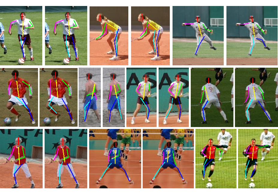
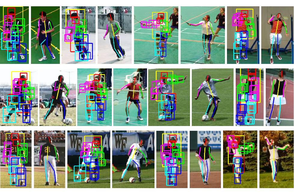
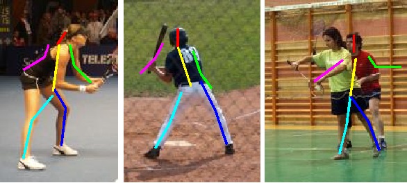
Fig. 4 displays our results on the LSP dataset. The left image in each pair denotes the detection results for single and combine parts, and the right is the fitted skeleton. Fig. 5 shows the comparison between [4] (left) and our method (right). We also show some failure examples in Fig. 6.

We compared the detection accuracy of our method with Yang & Ramanan [6], Johnson & Everingham [3], and Tian et al. [1] respectively. Table 1 summarizes the evaluation results and highlights the highest scores.

Compared to Yang & Ramanan [6], our results are better. Our detection accuracies on Upper Leg ($74.0\%$), Lower Leg ($69.8\%$), and Total ($62.8\%$) are consistently higher. Our performance is also superior to Johnson & Everingham [3]. We are aware of their later method [17], which achieved $62.7\%$ in total accuracy, but they trained their model on 11000 samples and relabeled the training set during optimization.

Recently, Tian et al. [1] suggested to partition all the 1000 training images into 5 disjoint training sets, and the detection accuracy is defined as the maximal score of 5 models. This approach is practical, because the evaluation method in [16] prompts the algorithms that report more candidate detections. With this evaluation bias, our method still marginally outperforms theirs. We further report our detection results using the first 200 training images ($6^{th}$ row) for fair comparison.

This experiment suggests our method outperformed the state of the art. This is possibly because we effectively exploit the connections between single and combined parts, as well as the benefit from exact inference.

4.2 Cross dataset validation

Experiment setting

We further investigate the generalization power of our model by cross dataset validation. One may speculate that our combined parts may be overfitted to a dataset, because they captures the distinctive features as HOG templates during visual category learning. This experiment suggests that our model is able to generalize to different dataset.

We trained our model on all the 305 images in the PARSE dataset [6], and then used the models to estimate human pose on the LSP dataset. We manually relabeled the LSP dataset for the purpose of testing, because its definition of left/right is based on human coordinate while the PARSE dataset is based on image coordinate. We used the same setting for Yang & Ramanan [4].

Figure 6: Failure examples of our method in the LSP dataset.

Figure 7: Examples of our method on the dog dataset from Pascal 2009. Top images: detection results for head (magenta), foreleg (green and blue). Bottom images: fitted skeleton after inference.

Results

The last two rows in Table 1 shows the detection accuracies of both algorithms. Compared to the $7^{th}$ row and $9^{th}$row, the performance of our model does not degrade, and surprisingly produce higher accuracy in some parts. As a result, our method empirically outperformed [4] in four out of six joints, and the Total accuracy is $5\%$ higher. Therefore, we conclude that the combination of mixed types facilitate inference process, and avoid overfitting in datasets.

4.3 Pascal VOC dog dataset

We tested our method on dog images from the PASCAL 2009 dataset. Bourdev et al. [9] annotated these images with up to 26 keypoints, but not all images have all annotations. In our experiment, we select 280 images that have at least the following 9 keypoints, namely, “nose”, left and right “eye”, “ear base”, “front elbow”, and “front paw”, respectively.

Experiment setting

In this experiment we used 3 combined parts, “head”, “left leg”, and “right leg”. We used 6 visual categories for each combined part. 100 images were used for training and the remaining for testing. We compared our method to [4] in this experiment. In the Yang & Ramanan [4], we used the 9 keypoints in a natural skeleton structure to build the tree model.

Method	Head	L.F.Leg	R.F.Leg	Legs	Total
[4]	56.1	52.8	58.3	55.6	55.7
Ours	52.8	60.6	63.3	62.0	58.9

Table 2: Results on the dog images, a subset of the VOC challenge.

Results

Fig. 7 shows some typical results in this experiment. The images on top is the detection results and the ones in bottom contain the fitted skeletons for dogs. This subset of the VOC dataset is very challenging, because the large variations in dog poses and camera viewpoints. Therefore, both [4] and our algorithm have low accuracies (Table. 2).

Although our performance is worse in the “head”, our detection on the “left fore leg” and the “right fore leg” are higher ($60.6\%$ and $63.3\%$, respectively). An average accuracy for legs is approximately $6\%$ higher than that of [4], and the total accuracy is $3\%$ higher. This experiment demonstrates that our method serves as a very good tool for modeling parts in other articulated objects such as animals.

5 Conclusion

This paper addressed three questions in human pose estimation using deformable models. Latent tree models are learned to approximate the joint distributions of body part locations, and single and combined parts are used together for effective inference. Empirical results suggest that our approach outperforms the state of the art in human pose and animal pose estimation.

References

- [1] Y. Tian, C. Lawrence Zitnick, and Srinivasa G. Narasimhan, “Exploring the spatial hierarchy of mixture models for human pose estimation,” in ECCV (5), 2012, pp. 256–269.
- [2] Y. Wang, D. Tran, and Z. Liao, “Learning hierarchical poselets for human parsing,” in Computer Vision and Pattern Recognition (CVPR), 2011 IEEE Conference on. IEEE, 2011, pp. 1705–1712.
- [3] S. Johnson and M. Everingham, “Clustered pose and nonlinear appearance models for human pose estimation,” in Proceedings of the British Machine Vision Conference, 2010, doi:10.5244/C.24.12.
- [4] Y. Yang and D. Ramanan, “Articulated pose estimation with flexible mixtures-of-parts,” in Computer Vision and Pattern Recognition (CVPR), 2011 IEEE Conference on. IEEE, 2011, pp. 1385–1392.
- [5] P. F. Felzenszwalb and D. P. Huttenlocher, “Pictorial structures for object recognition,” Int. J. Comput. Vision, vol. 61, no. 1, pp. 55–79, Jan. 2005.
- [6] D. Ramanan, “Learning to parse images of articulated bodies,” Advances in Neural Information Processing Systems, vol. 19, pp. 1129, 2007.
- [7] M. Everingham, L. Van Gool, C. K. I. Williams, J. Winn, and A. Zisserman, “The PASCAL Visual Object Classes Challenge 2009 (VOC2009) Results,” http://www.pascal-network.org/challenges/VOC/voc2009.
- [8] N. Dalal and B. Triggs, “Histograms of oriented gradients for human detection,” in Computer Vision and Pattern Recognition, 2005. CVPR 2005. IEEE Computer Society Conference on. IEEE, 2005, vol. 1, pp. 886–893.
- [9] L. Bourdev, S. Maji, T. Brox, and J. Malik, “Detecting people using mutually consistent poselet activations,” Computer Vision–ECCV 2010, pp. 168–181, 2010.
- [10] M. Sun and S. Savarese, “Articulated part-based model for joint object detection and pose estimation,” in Computer Vision (ICCV), 2011 IEEE International Conference on. IEEE, 2011, pp. 723–730.
- [11] M. J. Choi, V. Tan, A. Anandkumar, and A. S. Willsky, “Learning latent tree graphical models,” J. Mach. Learn. Res., vol. 12, pp. 1771–1812, July 2011.
- [12] C. Chow and C. Liu, “Approximating discrete probability distributions with dependence trees,” Information Theory, IEEE Transactions on, vol. 14, no. 3, pp. 462–467.
- [13] P. F. Felzenszwalb, R. B. Girshick, D. McAllester, and D. Ramanan, “Object detection with discriminatively trained part-based models,” Pattern Analysis and Machine Intelligence, IEEE Transactions on, vol. 32, no. 9, pp. 1627–1645, 2010.
- [14] S. Divvala, A. Efros, and M. Hebert, “How important are deformable parts in the deformable parts model?,” CoRR, vol. abs/1206.3714, 2012.
- [15] B. Sapp, A. Toshev, and B. Taskar, “Cascaded models for articulated pose estimation,” in ECCV (2), 2010.
- [16] V. Ferrari, M. J. Marín-Jiménez, and A. Zisserman, “Progressive search space reduction for human pose estimation,” in CVPR, 2008.
- [17] S. Johnson and M. Everingham, “Learning effective human pose estimation from inaccurate annotation,” in CVPR, 2011, pp. 1465–1472.