Translating Relational Queries into Spreadsheets

Abstract

Spreadsheets are among the most commonly used applications for data management and analysis. Perhaps they are even among the most widely used computer applications of all kinds. They combine in a natural and intuitive way data processing with very diverse supplementary features: statistical functions, visualization tools, pivot tables, pivot charts, linear programming solvers, Web queries periodically downloading data from external sources, etc. However, the spreadsheet paradigm of computation still lacks sufficient analysis.

In this article we demonstrate that a spreadsheet can implement all data transformations definable in SQL, without any use of macros or built-in programming languages, merely by utilizing spreadsheet formulas. We provide a query compiler, which translates any given SQL query into a worksheet of the same semantics, including NULL values.

Thereby database operations become available to the users who do not want to migrate to a database. They can define their queries using a high-level language and then get their execution plans in a plain vanilla spreadsheet. No sophisticated database system, no spreadsheet plugins or macros are needed.

The functions available in spreadsheets impose severe limitations on the algorithms one can implement. In this paper we offer $O(n\log^{2}n)$ sorting spreadsheet, but using a non-constant number of rows, improving on the previously known $O(n^{2})$ ones.

It is therefore surprising, that a spreadsheet can implement, as we demonstrate, Depth-First-Search and Breadth-First-Search on graphs, thereby reaching beyond queries definable in SQL-92.

1 Introduction

Spreadsheets are the desktop counterpart of databases and OLAP in enterprise-scale computing. They serve basically the same purpose — data management and analysis, but at the opposite extreme of the data quantity scale.

Spreadsheets are very popular, and are often described as the very first “killer app” for personal computers. Today they are used to manage home budgets, but also to create, manage and examine extremely sophisticated models and data arising in business and research.

In his keynote talk [1] during SIGMOD 1998 Bill Gates spoke about the role and challenges for spreadsheets:

A lot of users today find the true databases complex enough that they simply go into either the word processor, with the table-type capabilities, or into the spreadsheet, which I’d say is a little more typical, and use that as their way of structuring data.

And, of course, you get a huge discontinuity because, as you want to do database-type operations, the spreadsheet isn’t set up for that.

And so then you have to learn a lot of new commands and move your data into another location.

What we’d like to see is that even if you start out in the spreadsheet, there’s a very simple way then to bring in software that uses that data in a richer fashion, and so you don’t see a discontinuity when you want to move up and do new things.

But that’s very easy to say that. It’s going to require some breakthrough ideas to really make that possible.

Despite that encouragement, relatively little research has been devoted to spreadsheets and consequently they are still poorly understood. In particular, 16 years later Excel users show up at community forums asking for help in performing database operations on their spreadsheet data [2, 3, 4, 5, 6].

Probably the same group of users is the target of Google. Their spreadsheets have a very useful QUERY function. It is used to run Google Visualization API Query Language queries across data[7]. The on-line help provides the following example formula:

=QUERY(’Example Data’!$A$2:$H$7, "select B, MAX(D) group by B").

However, this function does not permit joining relations, and is incompatible with other spreadsheet systems.

The second notable fact is that spreadsheet language of formulas of Excel has become a de facto standard. It is implemented in a large number of spreadsheet systems, available for all major operating systems and hardware platforms, starting from handholds and ending in the cloud, from proprietary to open source.

Computer applications in the form of formula-only spreadsheets are therefore highly portable, probably to the extent comparable with Java bytecode. From this perspective, spreadsheet systems can be regarded as virtual machines, offered by various vendors, on which spreadsheet applications can be run.

It is therefore extremely surprising that those machines are predominantly programmed manually, with no compilers producing spreadsheet code from higher-level languages.

The main topic of this article is to offer a fully automated method to construct spreadsheet implementations for a wide class of relational data transformations. We have implemented all operators of relational algebra, including grouping and aggregations. On top of that, we also offer a tool to specify the transformations in a quite rich fragment of SQL. This is our answer to the challenge posed by Bill Gates: the discontinuity between spreadsheets and databases is reduced by the fact that the former have the ability to express relational queries, and the users of spreadsheets can perform relational data transformations in the spreadsheet itself.

In the same way we address also our second point: our tool is a compiler from a high-level language into the language of spreadsheet formulas. The full automation of the translation process reduces the number of human-introduced errors in the spreadsheet application, in which the spreadsheet formulas produced in the translation are used. As a result users can still work in the vanilla spreadsheet environment, benefit from high portability and other features like data analysis and visualisation, while the complex parts are generated by a tool that allows to express them in a better suited high level database vocabulary and avoids errors in complex computations.

2 The contribution

The present paper offers a twofold contribution.

It is an extended version of an earlier paper [8], which demonstrated as a “proof of concept”, that Excel (and other spreadsheets) are capable of storing and querying relational data, and can thereby serve as database engines. In that paper relational algebra was implemented in the spreadsheets.

Now we extend this claim by demonstrating an automated translator, capable of producing formulas-only spreadsheet implementations of queries written in SQL. And indeed, we treat a spreadsheet very much as a virtual machine, which provides a set of system functions, which we use to implement relational queries. The resulting worksheets are usually complex and their creation by hand could be cumbersome and prone to errors. Our compiler creates them without any human intervention. When compared to the earlier paper, we add a complete implementation of NULL values, according to the three-valued logic of SQL.

The functionalities of spreadsheets we utilize make our implementations work without using any plug-ins or macros.

The reader should bear in mind, however, that our claim of translating SQL queries into spreadsheets does not mean, that we can translate the algorithms typical RDBMS systems employ to implement SQL. In particular, most of the algorithms we use are of quadratic time complexity, and hence inefficient if used on large data sets. Moreover, our translation tool in its present form does not perform optimization.

Our investigation can also be understood as an inquiry into the computational power of spreadsheets. In this sense, we prove that they subsume the power of relational queries, although sometimes, as explained, above, by algorithms inferior than those usually employed in RDBMS. With this perspective in mind, we provide three additional, isolated elements, absent in the earlier paper [8].

One of them is an efficient sorting algorithm, implemented by spreadsheet formulas. The original sorting demonstrated in [8] was of quadratic time complexity. The present algorithm is $O(n\log^{2}n)$. Its drawback is that it requires $4\log n$ columns to sort $n$ items. Therefore we did not decide to use it in our automated SQL to spreadsheet translator, although 80 columns would already suffice to sort the largest number of columns of data, which can be stored in Excel 2013 — the newest one at the time of this writing. The other two algorithms we implement go beyond standard SQL. We present a recursive implementation of Breadth-First-Search for directed acyclic graphs, and an iterative implementation of Depth-First-Search for arbitrary graphs. This sheds some light on the real computational capabilities of spreadsheets, and their ability to express recursive queries.

As the model of spreadsheet syntax and semantics we take the Microsoft Excel^TM [9].

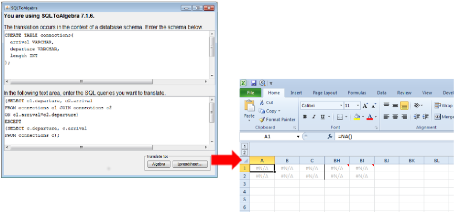
Figure 1: The idea of a database implementation in a spreadsheet. A Java program translates an SQL query into an equivalent spreadsheet. Table definitions visible above are not translated, but determine numbers of columns of the input tables.

2.1 Application scenarios

We envisage the main group of potential users of our work to be characterized by the following:

• They are experienced and relatively proficient users of spreadsheets, mainly Microsoft Excel.

• They are approaching the limits of spreadsheet abilities.

• Either they are not yet ready to migrate to a database, or they do not want to migrate at all.

One of us (J.Ty.) was active at the MrExcel.com forum where users of Excel can exchange tips and solutions, performing a kind of participant observation. It has turned out that requests to help in joining datasets are not uncommon.

One type of requests for help comes from users who are aware of database operations and clearly state what they need, as in the threads [2, 6].

The other type of requests comes from users, who describe the operation they need in plain words, clearly demonstrating, that they do not know databases. The first discussion [3] concerns social research. Its initiator needs to self-join a table on employment in companies, to detect pairs who work together in the same company. This task can be very concisely formulated as a query in SQL or the relational algebra. The ability to compile such a query into Excel formulas will significantly reduce the amount of necessary user work. In the second discussion [5] a user needs to join two tables of sensor data: humidity and temperature, both keyed by date. This meteorological application amounts to a textbook outer join. Matching humidity and temperature records are to be identified and non-matched records are to be retained. Again, the formulation of this query in a high level language is short and precise. Once it gets compiled to Excel formulas, it solves the user problem. The topic of the third discussion [4] is the problem of assembling services from components. The requesting user needs to join an association table of components with the service table that relates services with components. This time the problem reduces to an interesting inner join that leads to a non-4NF result. However, it can be solved with an inner equijoin. Its formulation in SQL and compilation to spreadsheet formulas solves the problem very quickly. To summarize, real users do need to join Excel data tables in various ways (self-, outer-, inner-, non-NF). A compiler of queries can be a valuable ally in their efforts.

It is instructive to have a look at the thread [6]. The user wants help in performing a join, and wants to do that in MsQuery. However, the Excel-only solution turns out to require just two formulas per data sheet and few clicks. If implemented with only formulas (instead of removing duplicates by a built-in Excel menu), it would become more complex, but still perfectly doable while the formulas would automatically recalculate without additional clicking, if the input data would change.

2.1.1 Spreadsheet to database migration?

We should explain why we think it makes sense to extend capabilities of spreadsheets by database functionalities, what we do here, instead of advising the users to migrate to a fully fledged database.

The reason is that spreadsheets combine in a natural and intuitive way many very diverse features. Just to name a few, they offer pivot tables, pivot charts, statistical functions, linear programming solvers, Web queries periodically downloading data from external sources, visualization tools, etc., suitable for datasets of moderate size. Re-creating them after migration to a database would require installing several external applications, configuring them to achieve integration, resulting in a complex system, whose overall usability would most likely be worse than that of the initial spreadsheet.

Finally, spreadsheets are very portable, much more than any database system. Their unique way of combining the application code (in the form of spreadsheet formulas) and the data in one file, and the access to both from the common interface gives the user the ability to open, analyse and edit them almost everywhere.

2.1.2 Spreadsheet error rate reduction

The second possible use of our solutions is the automated creation of data transformation formulas for Excel spreadsheets. They can be inserted into existing spreadsheet applications, performing complex data manipulations.

Today many users create such formulas manually, which results in high error rates and incomprehensible spreadsheets. We believe, that a typical relational query, written in SQL or relational algebra, is significantly easier to create and understand than its spreadsheet implementation. From this point of view, translating queries into the language of spreadsheet formulas is translating a higher-level language into a lower-level one.

Relational transformations can also be used to asses and improve the quality of data in spreadsheets. Many well-known integrity constraints can be enforced by SQL queries. The same goal can be therefore achieved by spreadsheet translations of relational queries. If they are inserted to an existing spreadsheet, they can indicate violations of integrity constraints.

2.2 Related work

To the best of our knowledge, the problem of expressing relational algebra and SQL in spreadsheets has not been considered in the setting we adopt here prior to [8].

The following results are the most similar to our work. The article [10] proposes an extension of the set of spreadsheet functions by a carefully designed database function, whereby the user can specify and later execute SQL queries in a spreadsheet-like style, one step at a time. These additional operators are executed by a classical database engine running in the background. Our contribution means that exactly the same functionality can be achieved by the spreadsheet itself. Two papers [11, 12] describe a project, later named Query by Excel to extend SQL by spreadsheet-inspired functionality, allowing the user to treat database tables as if they were located in a spreadsheet and define calculations over rows and columns by formulas resembling those found in spreadsheets. In the final paper [13] a spreadsheet interface is offered for specifying these calculations, which had to be specified in an SQL-like code in the earlier papers. Finally, [14] describes a method to allow RDBMs to query data stored in spreadsheets.

There is also a number of papers which discuss various methods to support high-level design of spreadsheets, in particular [15, 16, 17, 18, 19, 20, 21, 22, 23]. Some of them consider spreadsheets from the functional programming perspective.

2.3 Technicalities

We assume the reader to be basically familiar with spreadsheets. The present article is written to make the solutions compatible with Microsoft Excel, from version 2007 onward. This version introduced a number of new functions, absent in the earlier versions of Excel. They allowed us to simplify implementations of several operators, when compared to the conference paper [8], which offers solutions compatible with older versions of Excel.

3 Application example

Almost every present day bank offers its customers internet access to their accounts. One of the standard possibilities is the download of a list of all transactions on the account in a given period. Most typically it is an Excel file.

So let us assume a bank account owner who wants to do a serious analysis of their financial activities in the past year. First of all, probably they do not make on average more than 10 bank operations per day, which makes the data to consist of at most 4000 rows. Data of this size can be reasonably processed in a spreadsheet.

Details of the data organization will differ from country to country and from bank to bank, but certainly the following fields will be provided in the file with Transactions:

• Date of the transaction,

• Trans_type,

• Amount,

• Balance after transaction,

• Card_number (NULL in case of non-card operations),

• Address where the transaction took place.

Now the user has many options, how to process the data:

1. The query

   SELECT Address, count(Amount)
   FROM Transactions
   WHERE Trans_type=’ATM withdrawal’
   GROUP BY Address
   

   returns the list of addresses of ATM’s used together with the frequency of their use.

2. SELECT Card_number, sum(Amount)
   FROM Transactions
   WHERE Trans_type=’Card payment’
   GROUP BY Card_number
   

   returns the sums paid using each of the cards operating on the account.

3. If parents and children have accounts in the same bank, they can match allowances transferred by parents with their receipt by children,

   SELECT Card_number, sum(Amount)
   FROM Parent_Transactions t1 JOIN
        Child_Transactions t2
   ON t1.Amount=-t2.Amount AND
      t1.Date=t2.Date
   

4. Self-join can be used to match a transaction creating account overdraft (and therefore a loan from the bank) and its repayments. It is however difficult to provide an SQL query here, since it very much depends on the details how loan identifier is included in the descriptions of its repayments.

While the first two queries can be, in principle, expressed in Excel’s Pivot Table, the third and fourth query cannot be.

4 Translation of SQL to spreadsheet

4.1 Architecture of a database implemented in a spreadsheet

In this article, we disregard a number of minor issues arising in a practical implementation of the database operations in a spreadsheet. First of all, there is the obvious limitation on the number and sizes of relations, views and their intermediate results, imposed by the maximal available number of worksheets, columns and rows in the spreadsheet system at hand. Next, the size of the data values (integers, strings, etc.) is also limited. The variety of data types in spreadsheets is also restricted when compared to database systems.

The overall architecture of a relational database implemented in a spreadsheet is as follows. Given a specification of a query in SQL, its implementation is created by our query compiler, in the form of an .xlsx file. The resulting spreadsheet implementation of the query is a single worksheet, consisting of the necessary number of columns for the data tables and, next to them, the columns performing the computations. Initially there are always two rows of formulas, and the user is supposed to mark the second row of the formulas and fill with its content as many rows as necessary, taking into account the size of the relations to be processed and the expected size of the output. The first row should be left untouched, because sometimes it contains formulas which differ from those which fill the remaining rows.

The columns performing computations, and producing thereby intermediate results, are not supposed to be edited by the user.

When the user manually enters data into the tables, the automatic recomputation of the spreadsheet causes the output of queries to be computed and appear in the columns with the result.

We assume the semantics over fixed domains of integers, Booleans, texts, so that a relation is a set or multiset of tuples over these domains, in the form implemented in the spreadsheet software.

The representation of a relation $r$ of arity $n$ is a group of $n$ consecutive columns in a worksheet, whose rows contain the tuples in the relation. It is a crucial assumption, that the user data does not contain spreadsheet error codes. We use those codes in our implementation for representing special information, and they would have been misinterpreted, if present in the initial data.

The representation of an SQL query $Q$ of arity $m$ is a group of $m+l$ consecutive columns in a worksheet. Initial rows of those columns are filled with formulas. In the last $m$ columns those formulas should return either (a component of) a tuple in the result of $Q$, or #N/A! — the NO-DATA-NULL (see discussion in section 5.1 below). In the remaining $l$ columns the formulas calculate intermediate (auxiliary) results. A worksheet of this kind can be created by entering the formulas in the first and second row, and then filling the second row downward to span as many rows as necessary. This uniformity assumption means in particular, that the formulas are completely independent of the data they will work on.

In the following we will consider both set and bag (multiset) semantics of the relational algebra. In the first case, duplicate rows are not permitted in the relations and queries; in the latter they are permitted. However, even in the set semantics a spreadsheet representation of a relation may contain many null rows, i.e., ones filled with NO-DATA-NULL values.

Furthermore, the representation may be loose if null rows are interspersed with the tuples, or standard if all the tuples come first, followed by the null rows.

Consequently, we have loose-set, loose-bag, standard-set and standard-bag semantics. No matter which of the above semantics we have in mind, the result of the query appears exactly as if it were a table, and can be used as such. Now the only thing necessary to compose queries is to locate their implementations side by side in a single worksheet and change input column numbers in the formulas computing the outermost query, to agree with the column numbers of the outputs of the argument queries. Then the output columns of the argument queries become the intermediate results columns of the composition.

Therefore, queries represented in this way are compositional. We utilize this, implementing the usual operators of relational algebra from [24] in Excel, and then composing query plans of SQL queries from them. The list of implemented operators consists of the following:

• Sorting,

• Duplicate removal $\delta r$,

• Selection $\sigma_{\theta}r$,

• Projection $\pi_{i,j,\ldots}r$,

• Union $r\cup s$,

• Difference $r\setminus s$,

• Cartesian product $r\times s$,

• Grouping with aggregation $\gamma_{L,c}r$, where $L$ is any set composed from operators SUM, COUNT, AVG, MAX and MIN applied to the columns of $r$, and $c$ is a subset of the columns of $r$, over which we perform grouping,

• Two operations specific to spreadsheets, absent in [24]: error trapping and standardization (see Section 4.1).

Additionally, we have implemented two important operators, which can theoretically be defined using those listed above, but deserve independent implementations of much better performance.

• Semijoin $r\operatorname{\ltimes}_{\theta}s$, where $\theta$ is an equality of two columns.

• Join $r\operatorname{\bowtie}_{\theta}s$, where $\theta$ is an equality of two columns.

The present implementations of the operators make full use of COUNTIFS and SUMIFS functions, and would not work in the versions of the Microsoft spreadsheet older than 2007.

We consider the query compiler accompanying the present paper, and accessible from the Web page of the present paper (see Section 9), as the source of information about how the operators are implemented. An additional functionality present in the compiler is the mechanism for adapting the spreadsheet formulas to the number of columns in the input relations.

In the earlier paper [8] the operators were implemented using array formulas, to keep them compatible with Excel versions prior to 2007. The formulas were explained there in detail, and the present ones have not changed much.

Therefore we have decided to omit most of the descriptions of the basic operators in this paper. A few of them, which are of more interest, are described below in section 6.9.

4.2 Query compiler

Worksheets necessary to process queries composed of a single relational operator are rather complex. In case of queries composed from multiple operators and especially multi-way joins, resulting Excel formulas are almost intractable for humans. Therefore, an application of the described technology by typical clerks is hardly possible. In order to cater for their needs we have developed a compiler of queries. The compiler is implemented in Java. The user can define his/her query in SQL. The input consists of the query itself and of the CREATE TABLE statements for the used tables. Their purpose is to determine the number of columns of the input.

For each query, the compiler produces an empty worksheet that implements the given query.

The compilation is performed in two steps.

1. SQL is translated into a relational algebra expression, according to the algorithm described in [25].

2. This relational algebra expression is translated into a spreadsheet, using Excel implementations of all operators of the relational algebra, i.e. the projection, the selection, the equijoin, the Cartesian product, grouping, basic aggregates (sum, min, max, average, count), duplicate removal, sorting and set operations (union, difference and intersection).

Both steps are valid for the set semantics of SQL. This means that the result of an SQL query and its spreadsheet implementation resulting from the compilation, given identical tables as inputs, will produce exactly the same sets of tuples.

However, the first step in the translation is not valid for the bag semantics, if the query contains nested related subqueries. For such queries the sets of tuples in the bag semantics and in the spreadsheet will be the same, but their multiplicities may differ.

The first step is valid for the bag semantics, when applied to simple queries, which do not contain nested subqueries. This is discussed e.g. in [26] where a multi-set relational algebra has been defined. Furthermore, the authors have shown that a number of rewrite rules that work for the classic set algebra hold also in the bag algebra. They have also given examples of “set” rules that do not migrate to the bag setting. The article [26] proves that a translation of SQL queries to algebra expressions is feasible, however it does not present a ready-to-implement algorithm to do so. Since the article [25] offers such an algorithm (but only for the set semantics), we have decided to use it. This paper is in fact devoted to the translation of SQL statements to Excel worksheets. Therefore, we have assumed that the peculiarities of bag and set semantics are a minor issue.

We illustrate the operation of our compiler using an example query. Assume a database table connections on railway connections. Each of its rows describes a directed connection from the station departure to the station arrival of the given length. We distinguish columns in algebra expressions by their indexes. Therefore we reference departure as 1, arrival as 2 and length as 3.

Let us identify pairs of stations that are not connected directly, but the travel between them requires one change. In SQL we can formulate this as the self join presented in Fig. 2.

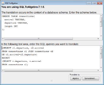
Figure 2: SQL to spreadsheet compiler interface.

The first result is translation of this query into the relational algebra, which can be on demand shown to the user in the following form:

DiffSet(
   Project(
      EqJoin(
         Reference(connections),
         Reference(connections),
         2,1
      ),
      [2, 4]
   ),
   Project(
      Reference(connections),
      [1, 2]
   )
)

The user can also request a translation of the query into an Excel workbook, yielding the result shown in Figures 3 and 4. The latter spreadsheet results from filling the former one for the desired number of rows and inserting the data. The user should fill sufficiently many rows to accomodate the largest intermediate results created in the computation process. The possibility to view the algebra expression corresponding to the SQL query can be helpful in estimating that number.

Cells in the first row contain comments, indicated by small red triangles. The spreadsheet cell comments provide a very basic explanation what the formulas compute – indeed they identify the relational algebra operator they implement and the columns which are inputs to that operator.

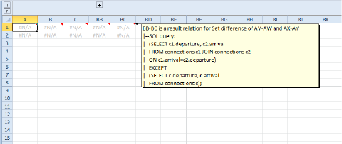
Figure 3: Spreadsheet implementation of the SQL query from Fig. 2. Hovering over a cell with a small red triangle displays description of the column it belongs to. Columns between C and BB hold intermediate results and are hidden by default.

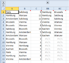
Figure 4: Spreadsheet implementation of the SQL query from Fig. 2 filled to 15 rows, with sample data and output consisting of 3 tuples.

5 Practical Level

This part is devoted to the discussion of the implementation issues of our translator.

5.1 NULL values

NULL values are unavoidable in practical implementations of relational databases. They lead to a three-valued logic that also has to be implemented. Analogously to many programming environments, spreadsheets do not have any feature that can be easily adopted as the database NULL. Therefore we offer an implementation of NULL. We will call it NO-VALUE-NULL.

However, we must start with NO-DATA-NULL, which does not exist in standard databases, and should not be confused with NO-VALUE-NULL. Indeed, the specific feature of our implementation of database queries in Excel is that they always process a fixed number of rows of the input tables. It does not matter how many of them are actually occupied by data. Hence, we must distinguish between NO-DATA-NULL that means “there is no row of data here” and the quite different NO-VALUE-NULL meaning “there is a row of data here, but this attribute has no value”.

Our choice is to represent NO-DATA-NULL by the error #N/A! which is generated by the function NA(). It has a corresponding test function ISNA() that returns TRUE if the argument is or evaluates to #N/A! and FALSE otherwise. The advantage of this representation is that in many particular Excel formulas we use, #N/A! is the natural outcome meaning that there should be no data row at this location.

For NO-VALUE-NULL we use #VALUE! generated with =INDEX(0,-1). It has the test ISERR(), i.e. a function which returns TRUE if the argument is any error except #N/A! and FALSE otherwise. Unfortunately, this NULL does not behave exactly according to Kleene rules when logical connectives are applied to it. Therefore, it requires coding of logical connectives in the queries. However, the test =#VALUE!=#VALUE! returns #VALUE!, as desired.

Hence, our two NULL representations behave as desired. Both of them have functions that create them and tests that distinguish them. Those two NULLs are supported in the query compiler, which we describe next.

6 Algebra Implementation

6.1 R1C1 notation

In the following we use the row-column R1C1-style addressing of cells and ranges, supported by Excel. This notation is easier to handle in a formal description, although in everyday practice the equivalent A1 notation is dominating and probably easier to understand. Therefore our translator produces worksheets in the A1 notation. A user who wants to see them in the R1C1 notation must change the appropriate setting in the Excel options. The key advantage of the R1C1 notation becomes evident when we enter a formula into a cell, click a small handle in the lower right corner of it and extend its boundaries either horizontally or vertically. This operation results in copying the content of the initial cell to the new, larger area of the worksheet. In the R1C1 notation the formulas resulting from filling are identical to the initial one, which makes our explanations in the paper much simpler.

In the R1C1 notation, both rows and columns of worksheets are numbered by integers starting from 1. For arbitrary nonzero integers $i$ and $j$ and nonzero natural numbers $m,n$ the following expressions are cell references in the R1C1 notation: RmCn, R[i]Cm, RmC[j], R[i]C[j], RCm, RC[i], RmC, R[i]C. The number after ‘R’ refers to the row number and the number after ‘C’ to the column number. If that number is missing, it means “same row (column)” as the cell in which this expression is used. A number written in square brackets is a relative reference and the cell to which this expression points should be determined by adding that number to the row (column) number of the cell in which the reference is used. A number without brackets is an absolute reference to a cell whose row (column) number is equal to that number. For example, R[-1]C7 denotes a cell which is in the row directly above the present one in column 7, while RC[3] denotes a cell in the same row as the present one and 3 columns to the right. If R or C is itself omitted, the expression denotes the whole column or row (respectively), e.g., C7 is column number 7.

Below we discuss the most important elements of Excel we use, but this presentation is not exhaustive: we sometimes use functions not presented below.

6.2 IF function

IF is a conditional function in spreadsheets. The syntax is

IF(condition,true_branch,false_branch).

Its evaluation is lazy, i.e., after the condition is evaluated and yields either TRUE or FALSE, only one of the branches is evaluated. It can be therefore used to protect functions from being applied to arguments of wrong types, trap errors, and, last but not least, to speed up execution of queries by avoiding computation of certain branches.

6.3 MATCH and INDEX functions

We mostly use MATCH using the syntax MATCH(cell,range,0). It returns the relative position of the first value in range which is equal to the value in cell, and an #N/A! error if such a value does not appear there.

A call MATCH(range,cell,1) is correct only if range is sorted in ascending order. Then, such a call to MATCH returns the relative position of the largest value in range that is less than or equal to the value in cell.

INDEX is used in the syntax INDEX(range,cell). This function call returns the value from range whose relative position is given by the value from cell.

6.4 COUNTIFS

In Excel 2007 two new highly expressive functions COUNTIFS and SUMIFS appeared for the first time. The function COUNTIFS counts rows (columns, resp.) satisfying multiple criteria, which can refer to several columns (rows, resp.). The general syntax is

COUNTIFS(rng₁,cr₁,…,[rng_k,cr_k]),

where each of the ranges rng has the same dimension.

If the input ranges are columns, the function returns the number of rows $r$ such that the $r$th value in column_i satisfies criterion cr_i for $i=1,\ldots,k$. In the dual form, the calculation proceeds in the same way, except that rows take over the role of columns and vice versa.

For example, in the context of the worksheet depicted in Fig. 5, the formula

=COUNTIFS(RC1:R5C1,"<"&RC3,RC2:R5C2,R2C3)

returns 2, since there are two rows in the data, in which a number smaller than 3 is accompanied by the string "a". Note the way of creating criteria, which can be expressed by a string produced by concatenating (operator &) the inequality sign with the reference to the numerical argument, or by a value or reference, in which case the condition is, by default, equality.

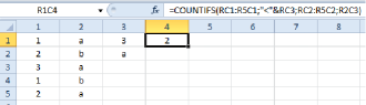
Figure 5: In the context of this worksheet the formula
=COUNTIFS(RC1:R5C1,"<"&RC3,RC2:R5C2,R2C3) returns 2.

6.5 SUMIFS

This time the syntax is

SUMIFS(sum_rng,rng₁,cr₁,…,[rng_k,cr_k]).

The operation of SUMIFS is quite similar to that of COUNTIFS, except that the rows are not counted, but the values in column sum_rng are summed over the rows satisfying the criteria.

6.6 ROW and COLUMN

The function call ROW() returns the row number in which the call is located. Similarly, COLUMN() returns the column number in which the call is located.

6.7 OFFSET

OFFSET is a function which differs significantly from all other functions mentioned in this paper. It allows the user to specify an arbitrary range of cells, whose location is determined by the numerical arguments of OFFSET. The syntax is

OFFSET(reference, rows, cols, [height], [width])

The call to this function yields a range, which is determined as follows: its top left corner is located rows down and cols to the right of reference. If no optional argument is provided, the range is a single cell, if they are present, they specify the dimensions of the range. The specific feature of OFFSET calls is that their arguments are calculated at runtime and only then it becomes known, what cell each OFFSET call refers to. In particular, when this function is used, it is impossible to determine, before executing the spreadsheet, if circular references are created or not.

6.8 Notation

We use the following convention for presenting our implementations:

COLUMNS 
=FORMULA
 

means that =FORMULA is entered into each cell of the COLUMNS, which may be specified either to be a single column (e.g. C5 ) or a range of a few columns (e.g. C5:C7), or a single cell (e.g. R1C5), and in each case belongs to the columns with intermediate values. In few cases we first fill a complete column with formulas, and then override the formula in the first row. This is used to create columns in which the first formula differs from those in the subsequent rows.

The notation

*COLUMNS 
=FORMULA
  indicates that formulas located in COLUMNS calculate the output of the query.

6.9 Relational algebra

In the examples presented here the arguments of the algebra operators are binary or ternary relations. Our query compiler uses parameterized forms of the implementations below, which work for any numbers of column in the input.

Except sorting, in all other cases we assume the input to be in the standard form, i.e., null rows are at the bottom.

We describe the following implementations, from the full list of [24]:

• Sorting;

• Grouping with aggregation $\gamma_{L,c}r$, where $L$ is any combination of operators SUM, COUNT, AVG, MAX and MIN applied to the columns of $r$ and $c$ is a subset of the columns of $r$;

• Semijoin $r\operatorname{\ltimes}_{\theta}s$, where $\theta$ is an equality of two columns;

• Join $r\operatorname{\bowtie}_{\theta}s$, where $\theta$ is an equality of two columns.

6.10 Sorting

Now we describe an implementation of sorting, used in our translator. It is of quadratic complexity. We describe a significantly faster sorting algorithm in section 7.1 below. However, it uses a non-constant number of columns, hence was not incorporated into the translator.

We assume that columns C1:C3 contain the source data and we sort in ascending order by the values in C1.

R1C4 
=COUNTA(C1)-COUNTIFS(C1,NA())
 

C5 
=IF(ISNA(RC1),R1C4+1,IF(ISERR(RC1),
1+R1C4-COUNTIFS(C1,RC1),
COUNTIFS(C1,"<"&RC1)+
COUNTIFS(R1C1:RC1,RC1)))
 

C6 
=MATCH(ROW(),C5,0)
 

*C7:C9 
=INDEX(C[-6],RC6)
 

For descending sort the only change is

C5 
=IF(ISNA(RC1),R1C4+1,IF(ISERR(RC1),
1+R1C4-COUNTIFS(C1,RC1),
COUNTIFS(C1,">"&RC1)+
COUNTIFS(R1C1:RC1,RC1)))
 

In either case, the formulas compute in RC5 the number of entries in column C1 which are smaller than or equal to RC1 plus the number of entries equal to RC1 in R1C1:RC1. This is the number of the row into which RC1 should be relocated during sort.

Now RC6 contains the number of the row in which the number of the present row appears in C5.

Finally, the formulas in RC7, RC8, RC9 fetch the values from columns C1, C2, C3 from the row calculated in RC6.

An important property of this operation is that this form of sorting is stable.

6.11 Grouping with aggregation

Grouping is an operator, whose implementation in the translator differs significantly from the one given in [8]. The reason is that the present one computes simultaneously many aggregates for one grouping, unlike the former one.

In the following, we assume that the relation to be processed is located in C1:C10. We wish to express the grouping, which in SQL can be declared as follows:

SELECT C1,C2,MIN(C3), MAX(C4), SUM(C5),
       COUNT(C6,C7), AVG(C8),
       COUNT(DISTINCT C9,C10)
FROM C1:C10
GROUP BY C1,C2

We have the following problems:

• For each separate grouping performed we leave one row from each group:

  • for MIN(C3) and MAX(C4) we leave the row where the actual minimum or maximum is attained;

  • for the remaining operators we leave the very first row of each group together with the computed aggregate.

• Now we may have between 1 and 3 entries for each group, with different aggregations, which must be unified to produce a single row with all aggregates.

C11 
=COUNTIFS(R1C1:RC1,RC1,R1C2:RC2,RC2)
 

This counts which occurrence of the values in C1:C2 we have in the present row.

C12 
=IF(ISNA(RC1),NA(),IF(ISERR(RC3),
COUNTIFS(C1,RC1,C2,RC2)-
COUNTIFS(C1,RC1,C2,RC2,C3,RC3),
COUNTIFS(C1,RC1,C2,RC2,C3,"<"&RC3)))
 

This is a help formula for minimum. It counts how many tuples in C1:C3 have the same values in C1:C2 as in the present row, and a smaller value in C3. There is a special treatment if there is NO-VALUE-NULL in C3.

C13 
=IF(ISNA(RC1),NA(),IF(ISERR(RC4),
COUNTIFS(C1,RC1,C2,RC2)-
COUNTIFS(C1,RC1,C2,RC2,C4,RC4),
COUNTIFS(C1,RC1,C2,RC2,C4,">"&RC4)))
 

This is an analogous formula for maximum.

C14 
=IFERROR(RC[-9],"")
 

C15 
=IFERROR(RC[-7],"")
 

These two formulas replace NULLs of both kinds by empty texts for SUM and AVG aggregations. The reason is that Excel’s SUMIFS function produces an error when one of its arguments is an error, but fortunately ignores text arguments.

C16 
=IF(AND(ISERROR(RC[-7]),
ISERROR(RC[-6])),INDEX(0,-1),
COUNTIFS(R1C1:RC1,RC1,R1C2:RC2,RC2,
R1C9:RC9,RC9,R1C10:RC10,RC10))
 

This help formula for COUNT DISTINCT counts which occurrence of the values in C1:C2,C9:C10 we have in the present row. Note that it produces NO-VALUE-NULL in case there are NULLs in columns C9:C10 of the present row.

*C17:C18 
=IF(RC11=1,RC[-16],NA())
 

This formula turns non-first occurrences of pairs from C1:C2 into NO-DATA-NULL. All subsequent formulas test if this value in NO-DATA-NULL and if so, become NO-DATA-NULL, too.

*C19:C20 
=IF(ISNA(RC17),NA(),
SUMIFS(C[-16],C1,RC1,C2,RC2,C[-7],0))
 

This formula relocates the minimum and maximum values (recognized by 0 in columns C12 and C13, resp.) into the present row.

*C21 
=IF(ISNA(RC17),NA(),
SUMIFS(C[-7],C1,RC1,C2,RC2))
 

This formula computes the SUM aggregation.

*C22 
=IF(ISNA(RC17),NA(),
COUNTIFS(C1,RC1,C2,RC2)-
COUNTIFS(C1,RC1,C2,RC2,
C[-16],INDEX(0,-1),
C[-15],INDEX(0,-1)))
 

This formula computes the COUNT aggregation, where double NO-VALUE-NULL values are not taken into account.

*C23 
=IF(ISNA(RC17),NA(),
SUMIFS(C[-8],C1,RC1,C2,RC2)/
COUNTIFS(C1,RC1,C2,RC2))
 

This formula computes the SUM aggregation.

*C24 
=IF(ISNA(RC[-7]),NA(),
COUNTIFS(C1,RC1,C2,RC2,C[-8],1))
 

This final formula computes the COUNT DISTINCT aggregate. The first occurrences are indicated by 1 in column C16.

6.12 Semijoin

Assume that we are given two relations located in C1:C2 and C3:C4, respectively, and we wish to compute the equisemijoin $\mathtt{C1:C2}\operatorname{\ltimes}_{\mathtt{C1}=\mathtt{C3}}\mathtt{C2:C3}.$

This is achieved in the following way. The two formulas below copy the rows from C1:C2, replacing those which do not belong to the semijoin by NO_DATA_NULLs. The resulting relation is loose and should be normalized.

C5 
=IF(ISERROR(MATCH(RC1,C4,0)),NA(),RC1)
 

C6 
=IF(ISNA(RC5),NA(),RC2)
 

6.13 Join

Let two relations be located in C1:C2 and C3:C4, respectively, and the equijoin $\mathtt{C1:C2}\operatorname{\bowtie}_{\mathtt{C1}=\mathtt{C3}}\mathtt{C3:C4}$ should be computed.

It is computed according to the decomposition

$$\mathtt{C1:C2}\operatorname{\bowtie}_{\mathtt{C1}=\mathtt{C3}}\mathtt{C3:C4}=$$

$$(\mathtt{C1:C2}\operatorname{\ltimes}_{\mathtt{C1}=\mathtt{C3}}\mathtt{C3:C4})\operatorname{\bowtie}_{\mathtt{C1}=\mathtt{C3}}(\mathtt{C3:C4}\operatorname{\ltimes}_{\mathtt{C3}=\mathtt{C1}}\mathtt{C1:C2})$$

Let us note that we have

$$\pi_{\mathtt{C1}}(\mathtt{C1:C2}\operatorname{\ltimes}_{\mathtt{C1}=\mathtt{C3}}\mathtt{C3:C4})=\pi_{\mathtt{C3}}(\mathtt{C3:C4}\operatorname{\ltimes}_{\mathtt{C3}=\mathtt{C1}}\mathtt{C1:C2}).$$

Then, denoting this the set of elements in this common projection by $X,$ we can further decompose the join into the sum

$$\bigcup_{x\in X}\{x\}\times\pi_{\mathtt{C2}}(\sigma_{\mathtt{C1}=x}(\mathtt{C1:C2}))\times\pi_{\mathtt{C4}}(\sigma_{\mathtt{C3}=x}(\mathtt{C3:C4})).$$

We will call the expressions $\{x\}\times\pi_{\mathtt{C2}}(\sigma_{\mathtt{C1}=x}(\mathtt{C1:C2}))\times\pi_{\mathtt{C4}}(\sigma_{\mathtt{C3}=x}(\mathtt{C3:C4}))$ blocks of the join.

The Excel implementation of the above idea is as follows.

The initial phase of computing the join consists of application of several other operators, according to Fig. 6.

Figure 6: The structure of equijoin of two relations stored in C1:C2 and C3:C4

After this initial phase, columns C27:C28 contain

$$\bigcup_{x\in X}\{\langle x,\mathrm{card}(\sigma_{\mathtt{C1}=x}(\mathtt{C1:C2}))\rangle\}$$

and columns C31:C32 contain

$$\bigcup_{x\in X}\{\langle x,\mathrm{card}(\sigma_{\mathtt{C3}=x}(\mathtt{C3:C4}))\rangle\}.$$

The real join creation takes place in columns C33:C42 and is executed as follows.

C33 
=MATCH(RC[-6],C[-25],0)
 

C34 
=MATCH(RC[-3],C[-21],0)
 

These two columns contain pointers to the first rows of the sorted input tables with consecutive elements of $X.$

C35 
=IFERROR(RC[-7]*RC[-3],"")
 

The values in C35 are the sizes of the blocks of the join.

C36 
=IFERROR(R[-1]C[-1]+R[-1]C,"")
 

R1C36 
=0
 

C36 contains the numbers of rows at which the consecutive blocks of the join should begin minus 1.

R1C37 
=SUM(C[-2])
 

This number is the total cardinality of the join to be produced.

C38 
=IF(ROW()>R1C37,NA(),
MATCH(ROW()-1,C36,1))
 

In this line function MATCH is used with the last parameter 1 to do inexact search for the number of the block from which the present tuple in join should originate.

C39 
=IF(ISNA(RC[-1]),NA(),
IF(RC[-1]<>R[-1]C[-1],1,1+R[-1]C))
 

R1C39 
=IF(ISNA(RC[-1]),NA(),1)
 

These two lines compute, within each block, the number of the present row of the join within its block.

*C40 
=INDEX(C[-13],RC[-2])
 

*C41 
=INDEX(C[-32],INDEX(C[-8],RC[-3])+
MOD(RC[-2]-1,INDEX(C28,RC[-3])))
 

*C42 
=INDEX(C14,INDEX(C34,RC[-4])+
QUOTIENT((RC[-3]-1),INDEX(C28,RC[-4])))
 

In the last three columns we fetch the right $x\in X,$ then the relevant element of $\sigma_{\mathtt{C1}=x}(\mathtt{C1:C2})$ and the relevant element of $\sigma_{\mathtt{C3}=x}(\mathtt{C3:C4}),$ creating that tuple of the join.

7 Special algorithms

The algorithms whose implementations we describe in this section are not used by the query compiler. They arose from our attempts to either find better algorithms for SQL-92, or to express computations which go beyond SQL-92.

7.1 Fast sorting

The solution to the problem of sorting presented in Section 6.10 is clearly a quadratic algorithm.

In this section we describe an efficient linearithmic implementation. We adopt the well-known bottom-up merge-sort algorithm and simulate a sorting network over the data range.

A spreadsheet with an implementation of our algorithm is available at the Web page of the paper (see Section 9). It includes two worksheets one with a condensed version with fewer columns per step and one with many auxiliary columns for easy human understandability. Below we refer to the latter spreadsheet.

In the first step, pairs of neighbouring cells are sorted. The next step leaves sorted quadruples, and so on, until the whole data range is sorted. Obviously, if $n$ items are to be sorted, $\log n$ steps are needed. In the spreadsheet model of computation we cannot reiterate values in a cell. Thus our fast sorting does not work in place, but rather uses a logarithmic number of columns, i.e. successive columns are needed for successive steps. Such an organization can be compared to a sorting network.

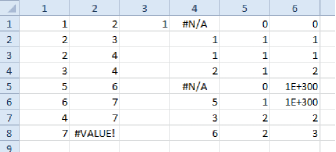
Figure 7: Spreadsheet implementation of the bottom-up merge sort algorithm in Excel. The area shown merges two already sorted 4-element blocks on the left to yield a sorted 8-element block on the right.

The fast sorting algorithm presented below is composed of 12 columns per one level of merging. In practical situation one may condense this to just 4 columns, replacing references to cells by formulas which are in those cells (this process we call inlining).

Now we describe one such block. Let us assume that the already sorted blocks of certain length are located in column C25. We want to produce sorted blocks of doubled size in column C37.

In order to sort $n$ items it is necessary to use $\log n$ such groups of columns. The already sorted blocks of the initial data are of size 1, and each group of columns merges pairs of already existing blocks to produce sorted blocks of duplicate size.

Now we start the description of such a group of 12 columns.

C26 
=QUOTIENT(COLUMN(),12)
  This column determines which level of merging is performed now.

C27 
=POWER(2,RC[-1])
  This column determines the sizes of blocks to be merged.

C28 
=QUOTIENT(ROW()-2,RC[-1]*2)*2*RC[-1]+1
  Now we determine where the top of the two blocks to be merged starts…

C29 
=RC[-1]+RC[-2]-1
  …and where it ends…

C30 
=RC[-2]+RC[-3]
  …and where the bottom block starts…

C31 
=RC[-2]+RC[-4]
  …and where it ends.

The following 5 columns do the merging, and now the pattern of references becomes more complicated. Formulas do not refer only to cells to the left, but also to values above them, in those 5 columns.

C32 
=IF(MOD(ROW()-2,RC[-5]*2)=0,
RC[-4],IF(R[-1]C[4],R[-1]C+1,R[-1]C))
  This column computes the position of the first not-yet-merged element from the top block. It either repeats the value R[-1]C directly above in the same column, or increments it by 1, depending on the value R[-1]C[4] one row above and 4 columns to the right, which determined if the value in (then) subsequent step should be taken from the top or bottom block. The initial test IF(MOD(ROW()-2,RC[-5]*2)=0… checks if this row starts a new merging of two new blocks; if it is so then the formula returns the top element of the new top block to be merged RC[-4].

C33 
=IF(MOD(ROW()-2,RC[-6]*2)=0,
RC[-3],IF(R[-1]C[3],R[-1]C,R[-1]C+1))
  Now we do the same for the bottom block.

The following two columns retrieve the data elements from the just determined positions.

C34 
=INDEX(C[-9],RC[-2]+1)
 

C35 
=INDEX(C[-10],RC[-2]+1)
 

C36 
=IF(RC[-4]>RC[-7],FALSE,
IF(RC[-3]>RC[-5],TRUE,RC[-2]<=RC[-1]))
  In this column the comparison RC[-2]<=RC[-1] determines which of the found values is smaller and should go now to the output, and the result is represented as a Boolean value, to be used in the following row of columns C32 and C33. The initial two tests verify if all values from one of the merged blocks have already been used and we should take a value from the other block, irrespectively of anything else.

C37 
=IF(RC[-1],RC[-3],RC[-2])
  And here the chosen element, smaller of the two, is appended to the result.

Concerning the complexity of this implementation, for sorting $n$ items it consists of $n$ rows of formulas, and logarithmic number of columns, $O(n\log n)$ formulas in total. The formulas in turn either access a constant number of neighbouring cells and, in some of the columns, call INDEX function to return a particular element from the input column of unsorted items. Theoretically, the complexity of this operation is $O(\log n),$ resulting in $O(n\log^{2}n)$ total complexity. However, tests we have performed indicate that the time necessary to execute INDEX in Excel does not depend on the number of data elements in the input range, so in practice our sorting works in $O(n\log n)$ time, for $n$ not exceeding the number of rows available in Excel.

7.2 Graph traversing

Graph traversing is a fundamental algorithmic operation. It appears as an important step in numerous graph algorithms. Its two most important variants are Breadth-First-Search (BFS) and Depth-First-Search (DFS).

We are going to demonstrate that both of them can be implemented in spreadsheets, with the restriction that BFS works for acyclic directed graphs, while DFS for arbitrary directed graphs. An implementation of BFS for cyclic graphs can be done similarly to DFS. However, we have decided to show the BFS version for acyclic graphs to simplify this algorithm and its presentation. Furthermore, as we will show, this gives us an unusual way to test if a directed graph is cyclic or not. This test is another evidence that the potential of the spreadsheet systems has not been well recognized yet.

Technically speaking, we will demonstrate, how to order vertices of a graph, given as a list of edges, exactly in the order in which BFS and DFS visit them.

In both cases, we assume that the input (directed) graph $G$ is specified by its set $E$ of directed edges, which are pairs of vertices. The vertex set $V$ is determined by the set of edges. We are also given a start vertex $s\in V$, from which the traversal begins.

7.3 Breadth-First-Search

The idea of the algorithm is that we assign a level $\mathrm{lv}(v)$ to each vertex $v\in V$.

• $\mathrm{lv}(s)=0$ for the source vertex $s$.

• For every vertex $v\neq s$ with no incoming edges $\mathrm{lv}(v)=\infty$.

• For every other vertex $v$, we define $\mathrm{lv}(v)=1+\min\{\mathrm{lv}(w)~{}|~{}\langle w,v\rangle\in E\}$ (assuming that $1+\infty=\infty$).

Every linear ordering of those vertices of $G$, which have finite value of $\mathrm{lv}$ and such that $\mathrm{lv}$ is non-decreasing, corresponds to some BFS traversal of the graph.

Sorting is doable in spreadsheets, as well as filtering, hence it is sufficient to show how to compute $\mathrm{lv}$.

We have one technical problem: $\infty$ is not present in spreadsheet arithmetic. Instead we use $10^{300}$, which is more than the number of particles in the visible part of the universe, and, by the definition of the level, the finite values of level cannot achieve this quantity. So it is a fully functional substitute of $\infty$ for our purpose.

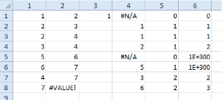
Figure 8: Spreadsheet implementation of the BFS graph traversal.

Now we discuss the implementation of our idea. We start with producing an expanded set of edges by adding to $E$ edges $\langle v,\mathtt{NULL}\rangle$ for all $v\in V$ with no outgoing edges. This modification does not alter the values of level resulting from the algorithm, and simplifies our task, since now every vertex appears as a first coordinate of some edge. This operation is expressible in SQL, hence it can be implemented in a spreadsheet, and we omit the formulas which perform it.

Next, we sort the expanded set of edges by the second coordinate. As a consequence the edges incoming into a vertex $v$ always form a contiguous block. Again we omit the formulas which perform the sorting (see Section 6.10).

Let the sorted edges of the expanded $E$ be provided row-wise in columns C1:C2 and the start node $s$ be located in cell R1C3.

Each row is therefore associated with an edge $\langle v,w\rangle$ located in columns C1:C2, and we are going to compute $\mathrm{lv}(v)$ in column C6.

We start by computing for each row corresponding to edge $\langle v,w\rangle$, the (position of the) beginning of the block of all edges incoming into $v$. If $v$ has no incoming edges, the result is #N/A!.

C4 
=MATCH(RC1,C3,0)
 

Next, for each row corresponding to edge $\langle v,w\rangle$, compute the number of edges of the expanded $E$ incoming into $v$.

C5 
=COUNTIF(C3,RC1)
 

The final column of formulas computes the levels of vertices. If the following formula is located in a row corresponding to an edge $\langle v,w\rangle$, it computes the level of $v$.

*C6 
=IF(RC1=R1C3,0,IF(ISERROR(RC3),1E300,
1+MIN(OFFSET(R1C6,RC4-1,0,RC5))))
 

First, the start vertex $s$ from R1C3 is assigned level 0. Next, if $v$ is not $s$ and has no incoming edges, its level becomes 1E300. If $v$ has incoming edges, OFFSET function creates a range in the present column, encompassing exactly all rows whose edges in columns C1:C2 have the form $\langle w,v\rangle.$ The formula then calculates MIN over this range and adds 1. This is the level of $v$ and its value is then recorded in columnC6. Since then it becomes available for computing levels of further vertices, allowing recursion. Note, that the acyclicity of $G$ implies that we do not get cyclic references and the computation is well-founded.

One can observe that the pattern of the references within column C5 reproduces exactly the expanded set of edges $E$ whose traversal we perform.

What remains to be done is to sort column C1 according to the value in C5, replace all vertices of level $\geq\mathtt{1E300}$ by #N/A! and finally eliminate the duplicates. Again, this is doable using relational operators.

An interesting observation is that such a spreadsheet can also perform the test if the input graph is acyclic, but in a quite specific way. A successful computation of the above spreadsheet determines that the graph is indeed acyclic. If it is not, the spreadsheet responds with a message that circular references are created.

cur_node:=s;
first_time:=true;
cur_parent:=NULL;
next_sibling:=NULL;
first_son:=the first son of cur_node;
visited:=<cur_node,first_time,cur_parent>;

repeat 2*|E| times
if first_time and first_son<>NULL
  then {move to the first son}
    cur_parent:=cur_node;
    cur_node:=first_son;
    first_son:=the first son of cur_node;
    first_time:=[cur_node does not appear in visited];
    visited:=append(visited,<cur_node,first_time,cur_parent>);
elseif next_sibling<>NULL and ((first_time and first_son=NULL) or not(first_time))
  then {move to the next sibling}
    cur_node:=next_sibling;
    first_son:=the first son of cur_node;
    first_time:=[cur_node does not appear in visited];
    visited:=append(visited,<cur_node,first_time,cur_parent>);
else {backtrack}
    cur_node:=cur_parent;
    cur_parent:=the parent of cur_node when cur_node was new, from visited;
    first_son:=the first son of cur_node;
    first_time:=[cur_node does not appear in visited];
    visited:=append(visited,<cur_node,first_time,cur_parent>);

Figure 9: The pseudo-code of the algorithm for DFS.

7.4 Depth-first-search

In an analogous situation, our present task is to determine the ordering of the vertices of $G$ in which they are discovered by DFS algorithm run on $G$ starting from $s$. We assume that the edges of $E$ are listed in some order. This order determines the relative order of the vertices reachable from any given vertex $v$.

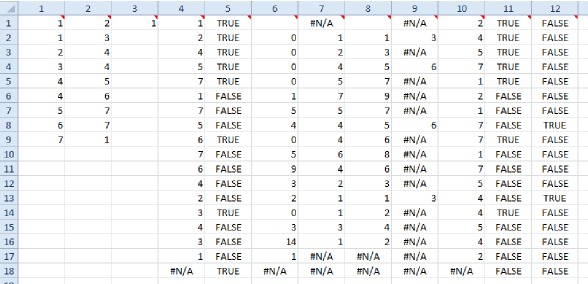
Figure 10: Spreadsheet implementation of the Depth-First-Search graph traversal.

Now, we describe the iterative algorithm which performs DFS. We will mimic its operation in a spreadsheet presented later, to determine the order in which it visits the vertices.

At all times the algorithm keeps the following information:

• the current vertex $\mathit{cur\_node}$,

• Boolean $\mathit{first\_time}$ which gives the information if the present visit to $\mathit{cur\_node}$ is the first one or not,

• the parent vertex $\mathit{cur\_parent}$ from which we have reached $\mathit{cur\_node}$,

• the $\mathit{first\_son}$ of $\mathit{cur\_node}$,

• the present $\mathit{next\_sibling}$ of $\mathit{cur\_node}$, which is the next vertex after $\mathit{cur\_node}$ among those reachable from $\mathit{cur\_parent}$,

• the list $\mathit{visited}$ of all tuples $(\mathit{cur\_node},\mathit{first\_time},\mathit{cur\_parent})$ encountered so far, in the order of appearance.

Each of the above vertices can be NULL. In Fig. 9 we present the pseudo-code of the algorithm for DFS. The body of its repeat statement is composed of a three-way conditional statement. Note that in all the three branches the last three statements are exactly the same. It is intentional, since this is not a classic “if” statement but a construction composed of three spreadsheet cells that implement the branches. Even if the factorisation of those three statements out of the conditional was feasible in traditional programming languages, it would complicate not simplify the resulting spreadsheet.

Since the number of iterations of the main loop is fixed, it is important to note what happens if the traversal is finished in fewer than $2*|E|$ steps: the algorithm then attempts to backtrack from the start vertex $s$ and makes $\mathit{cur\_node}$ NULL. From that moment on, whatever is computed from NULL results in NULL, so the rest of the output consists of NULLs.

This algorithm can be now translated into a spreadsheet. We do not need expanded $E$ for that purpose, since we do not touch unreachable vertices. The first step is to order the edges of $E$ by their first coordinate. This does not alter the relative order of children of the vertices. We omit the formulas which do the sorting (see Section 6.10).

The columns of the spreadsheet hold the values of variables of the above algorithm, each row corresponding to one iteration, and there are a few columns with auxiliary computations. Values of $\mathit{cur\_node}$ are stored in column C4, $\mathit{first\_time}$ in C5, $\mathit{cur\_parent}$ in C6, $\mathit{next\_sibling}$ in C8, $\mathit{first\_son}$ in C9. Columns C11 and C12 calculate the logical values of tests in the if …then and elseif …then statements of the algorithm, computed according to the values at the end of the iteration. Finally, column C13 holds numbers of consecutive rows, which helps in calculations.

First, $\mathit{cur\_node}$ is determined in column C4 depending on the logical tests computed at the end of the previous iteration.

*C4 
=IF(R[-1]C11,R[-1]C10,
IF(R[-1]C12,R[-1]C9,R[-1]C7))
 

The special formula in row 1 of that column is the initialization of $\mathit{cur\_node}$.

*R1C4 
=R1C3
 

The next column consists of formulas checking if the present value of $\mathit{cur\_node}$ appears in the history of that variable. MATCH returns an error when it is not.

C5 
=ISERROR(MATCH(RC4,R1C4:R[-1]C4,0))
 

The next column of formulas computes an auxiliary value: the row number of the first time the present value of $\mathit{cur\_node}$ was encountered. This first time is always distinguished by TRUE accompanying it in column C5. Because the present value of $\mathit{cur\_node}$ was a new one at most once, the sum of row numbers in column C13 yields the step number when it was new, or 0 if it was never new in the past (because it is new now).

C6 
=SUMIFS(R1C13:R[-1]C13,R1C4:R[-1]C4,RC4,
R1C5:R[-1]C5,TRUE)
 

We initialize this column by leaving the first cell empty.

R1C6 

 

Now we compute the value of $\mathit{cur\_parent}$ for the present $\mathit{cur\_node}$. In the case we are doing backtrack, the parent of $\mathit{cur\_node}$ is found in the history, by looking up the moment when $\mathit{cur\_node}$ was new. This position has been computed in RC6, and we take the corresponding value from the history of $\mathit{cur\_parent}$ in column C7.

C7 
=IF(R[-1]C11,R[-1]C4,IF(R[-1]C12,
R[-1]C7,INDEX(R1C7:R[-1]C7,RC6)))
 

For the start vertex in the first row we initialize $\mathit{cur\_parent}$ as NULL.

R1C7 
=NA()
 

Next we compute another auxiliary value: the number of the row of the input relation $E$ in which the edge $\langle\mathit{cur\_parent},\mathit{cur\_node}\rangle$ appears. It appears there exactly once, so again we sum the row numbers from column C13.

C8 
=SUMIFS(C13,C1,RC7,C2,RC4)
 

However, at the beginning the pair $\langle\mathit{cur\_parent},\mathit{cur\_node}\rangle$ is not an edge, so we initialize leaving the first cell in this column empty.

R1C8 

 

Referring to the auxiliary value computed in RC8, the following formula checks if in the edge of $E$ following $\langle\mathit{cur\_parent},\mathit{cur\_node}\rangle$ in the listing, the vertex $\mathit{cur\_parent}$ is still the parent. If it is so, the second coordinate of that edge is the present next sibling of $\mathit{cur\_node}$. Otherwise we set the next sibling to NULL.

C9 
=IF(INDEX(C1,RC8+1)=RC7,INDEX(C2,RC8+1),
NA())
 

Of course, the start vertex has no next sibling, so we initialize this column with NULL in the first row.

R1C9 
=NA()
 

In column C10 we find the first edge of $E$ whose first coordinate is the present $\mathit{cur\_node}$, and return the second coordinate as the first son $\mathit{first\_son}$ of $\mathit{cur\_node}$. If there is no such edge in $E$, $\mathit{first\_son}$ becomes NULL. This column does not require any specific initialization in the first row.

C10 
=IFERROR(INDEX(C2,MATCH(RC4,C1,0)),NA())
 

The last three columns compute the test results for if …then and elseif …then, to be used in the next iteration, and the row number.

C11 
=AND(RC5,NOT(ISNA(RC[-2])))
 

C12 
=AND(NOT(ISNA(RC8)),OR(NOT(RC5),
AND(RC5,ISNA(RC9))))
 

C13 
=ROW()
 

Now it is sufficient to remove duplicates from column C4 to get the order in which the initial algorithm discovers new vertices of the input graph. We omit the formulas for doing that.

7.4.1 Example application

The discussed graph traversal algorithms can be used to implement recursive queries over hierarchies. Hierarchical data is ubiquitous. In shops we have product categorization with some categories being subcategories of other. Companies have numerous corporate hierarchies of employees (manager-subordinate), organizational units (unit-subunit) or projects (project-subproject) etc. Although not covered in relational algebra, recursive queries to data representing hierarchies are often encountered in practice. In order to query such relations recursive queries have been introduced. First, they emerged in Oracle database in the form of the famous CONNECT BY clause, and then SQL:1999 adopted them as recursive common table expressions.

A spreadsheet with an example implementation of the described graph algorithms is available online as a supplementary material (see Section 9). The spreadsheet also includes an example of how the described techniques can be used to implement a typical query on the sample Oracle manager-subordinate hierarchy:

SELECT ename, level
FROM emp
START WITH empno = 7839
CONNECT BY PRIOR empno = mgr;

8 Conclusions, further research

We have demonstrated that SQL can be automatically translated into spreadsheet code, including NULL values. Thus, we have shown the power of the spreadsheet paradigm, which subsumes the paradigm of relational databases.

Apart from SQL, we have also implemented a few specific algorithms: a linearithmic sorting procedure and two graph traversing algorithms: BFS and DFS.

As the next steps:

• We plan to develop optimizations for SQL queries translated into spreadsheet.

• We plan to investigate whether spreadsheets can naturally implement other models of databases, like semi-structured or object-relational ones.

• Google spreadsheets provide the QUERY function, capable of expressing a limited fragment of SQL, as well as SORT, FILTER and UNIQUE functions, of similar roles. If a Google spreadsheet with those functions is downloaded as xlsx or ods file, these functions are not recognized by other spreadsheet systems and produce errors. We plan to use our implementations of algebra operators and experience with SQL translator to construct a translator capable of producing fully functional spreadsheet files from those downloaded from Google docs.

9 Software availability

The Web page of the present paper is hhtp://www.mimuw.edu.pl/~jty/Translating/, from which the software described in this paper can be accessed, including:

• the SQL to Excel translator, described in Section 4.2. This tool is independently accessible from Sourceforge http://sourceforge.net/projects/sqltoalgebra/?source=directory,

• Excel implementation of a sorting algorithm, working in time $O(n\log^{2}n)$, described in Section 7.1, and

• Excel implementations of BFS and DFS.

References

- [1] B. Gates, “Investing in research, SIGMOD Conference 1998 Keynote Speech, video,” ACM SIGMOD Digital Symposium Collection, vol. 1, no. 2, 1999.
- [2] SirMille. (2012, February) inner/outer/full join tables? [Online]. Available: http://www.mrexcel.com/forum/excel-questions/612236-inner-outer-full-jo%in-tables.html
- [3] xil. (2012, May) Connecting list of users with list of companies - please help. [Online]. Available: http://www.mrexcel.com/forum/excel-questions/704217-combining-two-lists%-into-one-big-list.html
- [4] stefanaalten. (2013, May) Combining two lists into one big list. [Online]. Available: http://www.mrexcel.com/forum/excel-questions/704217-combining-two-lists%-into-one-big-list.html
- [5] mzalikhan. (2012, Apr.) Double V-look up. [Online]. Available: \url{http://www.mrexcel.com/forum/excel-questions/625750-double-v-look-%up.html}
- [6] potter_ricky. (2014, March) Join two queries using msquery, returning into an excel workbook. [Online]. Available: http://www.mrexcel.com/forum/excel-questions/765490-join-two-queries-us%ing-msquery-returning-into-excel-workbook.html
- [7] G. Inc. (accessed 2014-05-21) Query Language Reference (Version 0.7). [Online]. Available: https://developers.google.com/chart/interactive/docs/querylanguage
- [8] J. Tyszkiewicz, “Spreadsheet as a relational database engine,” in Proceedings of the 2010 ACM SIGMOD International Conference on Management of data, ser. SIGMOD ’10. New York, NY, USA: ACM, 2010, pp. 195–206. [Online]. Available: http://doi.acm.org/10.1145/1807167.1807191
- [9] Microsoft Corporation. (accessed 2014/05/21) Excel Home Page - Microsoft Office Online. http://office.microsoft.com/en-us/excel-help/excel-functions-alphabetic%al-list-HA010277524.aspx?CTT=1.
- [10] B. Liu and H. V. Jagadish, “A spreadsheet algebra for a direct data manipulation query interface,” in ICDE ’09: Proceedings of the 2009 IEEE International Conference on Data Engineering. Washington, DC, USA: IEEE Computer Society, 2009, pp. 417–428.
- [11] A. Witkowski, S. Bellamkonda, T. Bozkaya, G. Dorman, N. Folkert, A. Gupta, L. Shen, and S. Subramanian, “Spreadsheets in RDBMS for OLAP,” in SIGMOD ’03: Proceedings of the 2003 ACM SIGMOD international conference on Management of data. New York, NY, USA: ACM, 2003, pp. 52–63.
- [12] A. Witkowski, S. Bellamkonda, T. Bozkaya, N. Folkert, A. Gupta, L. Sheng, and S. Subramanian, “Business modeling using SQL spreadsheets,” in VLDB ’2003: Proceedings of the 29th international conference on Very large data bases. VLDB Endowment, 2003, pp. 1117–1120.
- [13] A. Witkowski, S. Bellamkonda, T. Bozkaya, A. Naimat, L. Sheng, S. Subramanian, and A. Waingold, “Query by Excel,” in VLDB ’05: Proceedings of the 31st international conference on Very large data bases. VLDB Endowment, 2005, pp. 1204–1215.
- [14] L. V. S. Lakshmanan, S. N. Subramanian, N. Goyal, and R. Krishnamurthy, “On query spreadsheets,” in ICDE. IEEE Computer Society, 1998, pp. 134–141.
- [15] R. Abraham and M. Erwig, “Type inference for spreadsheets,” in PPDP ’06: Proceedings of the 8th ACM SIGPLAN Symposium on Principles and Practice of Declarative Programming. New York, NY, USA: ACM, 2006, pp. 73–84.
- [16] M. M. Burnett, J. W. Atwood, R. W. Djang, J. Reichwein, H. J. Gottfried, and S. Yang, “Forms/3: A first-order visual language to explore the boundaries of the spreadsheet paradigm,” J. Funct. Program., vol. 11, no. 2, pp. 155–206, 2001.
- [17] S. P. Jones, A. Blackwell, and M. Burnett, “A user-centred approach to functions in Excel,” in ICFP ’03: Proceedings of the Eighth ACM SIGPLAN International Conference on Functional Programming. New York, NY, USA: ACM, 2003, pp. 165–176.
- [18] M. Kassoff, L.-M. Zen, A. Garg, and M. Genesereth, “PrediCalc: a logical spreadsheet management system,” in VLDB ’05: Proceedings of the 31st international conference on Very large data bases. VLDB Endowment, 2005, pp. 1247–1250.
- [19] R. Mittermeir and M. Clermont, “Finding high-level structures in spreadsheet programs,” in WCRE ’02: Proceedings of the Ninth Working Conference on Reverse Engineering (WCRE’02). Washington, DC, USA: IEEE Computer Society, 2002, p. 221.
- [20] B. Ronen, M. A. Palley, and J. Henry C. Lucas, “Spreadsheet analysis and design,” Commun. ACM, vol. 32, no. 1, pp. 84–93, 1989.
- [21] D. Wakeling, “Spreadsheet functional programming,” J. Funct. Program., vol. 17, no. 1, pp. 131–143, 2007.
- [22] A. G. Yoder and D. L. Cohn, “Architectural issues in spreadsheet languages,” in Proceedings of the international conference on Programming languages and system architectures. New York, NY, USA: Springer-Verlag New York, Inc., 1994, pp. 245–258.
- [23] ——, “Real spreadsheets for real programmers,” in ICCL, H. E. Bal, Ed. IEEE Computer Society, 1994, pp. 20–30.
- [24] H. Garcia-Molina, J. D. Ullman, and J. Widom, Database System Implementation. Prentice-Hall, 2000.
- [25] J. V. den Bussche and S. Vansummeren, “Translating SQL into the relational algebra,” Lecture material, Universiteit Limburg, lecture INFO-H-417: Database Systems Architecture.
- [26] P. W. P. J. Grefen and R. A. de By, “A multi-set extended relational algebra - a formal approach to a practical issue,” in ICDE. IEEE Computer Society, 1994, pp. 80–88.