Diffusion of Interacting Particles in Discrete Geometries

Abstract

We evaluate the self-diffusion and transport diffusion of interacting particles in a discrete geometry consisting of a linear chain of cavities, with interactions within a cavity described by a free-energy function. Exact analytical expressions are obtained in the absence of correlations, showing that the self-diffusion can exceed the transport diffusion if the free-energy function is concave. The effect of correlations is elucidated by comparison with numerical results. Quantitative agreement is obtained with recent experimental data for diffusion in a nanoporous zeolitic imidazolate framework material, ZIF-8.

The equality of inertial and gravitational mass played a crucial role in Einstein’s discovery of general relativity. Similarly, Einstein’s work on Brownian motion is based on the identity of the transport- and self-diffusion coefficients for noninteracting particles Einstein (1905), leading eventually through Perrin’s experiments Perrin (1916) to the vindication of the atomic hypothesis. In general, however, diffusion of interacting particles is described by two different coefficients. The transport-diffusion coefficient $D_{t}$ quantifies the particle flux $j$ appearing in response to a concentration gradient $dc/dx$:

$$j=-D_{t}\frac{dc}{dx}.$$ (1)

The self-diffusion coefficient $D_{s}$ describes the mean squared displacement of a single particle in a suspension of identical particles at equilibrium: $\langle x^{2}(t)\rangle\propto D_{s}t$. An alternative way for measuring this coefficient is by labeling, in this system at equilibrium, a subset of these particles (denoted by $*$) in a way to create a concentration gradient $dc^{*}/dx$ of labeled particles under overall equilibrium conditions. The resulting flux $j^{*}$ of these particles reads:

$$j^{*}=-D_{s}\frac{dc^{*}}{dx}.$$ (2)

Both forms of diffusion have been studied in a wide variety of physical contexts, including continuum Tough et al. (1986); Anderson and Reed (1976); Van den Broeck et al. (1981); Van den Broeck (1985); Zwanzig (1992); Lucena et al. (2012); Nelissen et al. (2007); Carvalho et al. (2012) and lattice Gomer (1990); Ala-Nissila et al. (2002); Reed and Erlich (1981) models. Exact analytical results for the diffusion coefficient of interacting particles are however typically limited to a perturbation expansion, for example in the density of the particles. The effect of correlations is notoriously difficult to evaluate in continuum models, especially when hydrodynamic interactions come into play, while they can play a dominant role, for example, in lattice models with particle exclusion constraints.

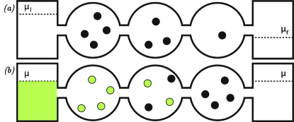
Figure 1: (Color online). The model: particles enter cavities via particle reservoirs at certain chemical potential. Particles jump between different cavities through narrow passages. $(a)$ Transport diffusion: a concentration gradient shows a current. $(b)$ Self-diffusion: a concentration gradient of labeled particles is introduced under overall equilibrium conditions.

In this Letter, we introduce a physically relevant model, for which exact analytical results can be obtained at all values of the concentration and for any interaction. It describes the diffusive hopping of interacting particles in a compartmentalized system, see Fig. 1 for a schematic representation. It is assumed that the relaxation inside each cavity is fast enough to establish a local equilibrium, described by a free-energy function characterizing the confinement and interaction of the particles. This model describes diffusion in confined geometries Burada et al. (2009). Of particular interest are microporous materials Davis (2002); Barton et al. (1999), which are widely used in industry, e.g. as catalysts in petrochemical industry and as water softeners. Because of their high thermal and chemical stability Park et al. (2006) and potential applications including carbon dioxide capture and storage Banerjee et al. (2008) and gas separation Bux et al. (2010), zeolitic imidazolate frameworks (ZIFs) have received considerable interest. As illustration, we compare our predictions with experimental results Chmelik et al. (2010) of diffusion of methanol in ZIF-8. At variance with previous experiments Jobic et al. (1999); Heinke et al. (2009); Salles et al. (2008); Rosenbach et al. (2008); Tzoulaki et al. (2009); Jobic (2008), it was found that the self-diffusion could exceed the transport diffusion, a result confirmed by molecular dynamics (MD) simulations Krishna and van Baten (2010a, b, c). We corroborate the observation that this phenomenon is due to clustering of the particles, and provide an analytical argument and a simple interpretation for the inversion. Our model in fact allows us to reproduce, in a quantitative way, the loading dependence of the self- and transport diffusion for different interactions. Finally, we mention that our model also serves an educational purpose, as the distinction between the transport- and self-diffusion coefficients and the role and contribution of the correlations therein, can be identified explicitly.

The model consists of a one-dimensional array of pairwise connected cavities, with particles entering in the outer left and right cavities from reservoirs at chemical potentials $\mu_{l}$ and $\mu_{r}$ respectively (see Fig. 1). The entire system is at temperature $T$. Particles stochastically jump between cavities by moving through narrow passages. These transitions occur on a slow time scale compared to the relaxation time inside each cavity, ensuring that an equilibrium distribution is effectively maintained in each cavity. It is described by a free energy $F(n)=U(n)-TS(n)$, with $n$ the number of particles in the cavity, $U(n)$ the energy and $S(n)$ the entropy. Furthermore, the dynamics is Markovian with a transition rate which has to reproduce the thermal equilibrium state $p^{\mathrm{eq}}$, when a cavity is connected to a single reservoir at chemical potential $\mu$:

$$p^{\mathrm{eq}}_{n}(\mu)=(\mathcal{Z})^{-1}e^{-\beta\left[F(n)-\mu n\right]},$$ (3)

with $\beta=(k_{B}T)^{-1}$ and ${\mathcal{Z}}^{-1}$ the normalization constant.

We first derive an exact expression for $D_{t}$ and $D_{s}$, in a limiting situation where correlations between particle numbers in different cavities are absent (see also supplementary material sup ). Consider a system consisting of three cavities, with $n_{l}$, $n$ and $n_{r}$ specifying the number of particles inside the left, middle and right cavity, respectively. In the limit in which the exchange rates with the middle cavity are small compared to the exchange rates with the reservoirs, the left and right cavity are effectively decorrelated from the middle cavity, and are characterized by the equilibrium probability distribution $p^{\mathrm{eq}}_{n_{l}}(\mu_{l})$ and $p^{\mathrm{eq}}_{n_{r}}(\mu_{r})$, respectively. This setup allows us to obtain exact analytical results at arbitrary particle density. The probability distribution $p_{n}$ for the middle cavity obeys the following master equation:

$$\dot{p}_{n}=k^{+}_{n-1}p_{n-1}+k^{-}_{n+1}p_{n+1}-\left(k^{+}_{n}+k^{-}_{n}\right)p_{n},$$ (4)

with $k^{+}_{n}$ and $k^{-}_{n}$ the rates to add or remove a particle from the middle cavity containing $n$ particles:

$$k^{+}_{n} =\sum_{n_{l}}p^{\mathrm{eq}}_{n_{l}}(\mu_{l})k_{n_{l}n}+\sum_{n_{r}}p^{\mathrm{eq}}_{n_{r}}(\mu_{r})k_{n_{r}n}$$ (5)

$$k^{-}_{n} =\sum_{n_{l}}p^{\mathrm{eq}}_{n_{l}}(\mu_{l})k_{nn_{l}}+\sum_{n_{r}}p^{\mathrm{eq}}_{n_{r}}(\mu_{r})k_{nn_{r}}.$$ (6)

The rate $k_{nm}$ denotes the probability per unit time for a particle to jump from a cavity containing $n$ particles to a neighboring cavity containing $m$ particles. At this stage we do not need to specify its explicit form, but we request that it obeys detailed balance:

$$k_{nm}/k_{m+1,n-1}=e^{-\beta\left[F(m+1)+F(n-1)-F(n)-F(m)\right]}.$$ (7)

The particle flux and concentration difference between the left and middle cavity read:

$$j(\mu_{l},\mu_{r}) =\sum_{n,n_{l}}\left(k_{n_{l}n}-k_{nn_{l}}\right)p^{\mathrm{eq}}_{n_{l}}(\mu_{l})p_{n},$$ (8)

$$dc(\mu_{l},\mu_{r}) =\left(1/\lambda\right)\sum_{n,n_{l}}(n-n_{l})p^{\mathrm{eq}}_{n_{l}}(\mu_{l})p_{n},$$ (9)

where $\lambda$ is the center-to-center distance between cavities. The transport diffusion $D_{t}$, quantifying the linear response of $j$ with respect to $dc$, is found from the ratio $-j/(dc/\lambda)$ in the limit $\delta=(\mu_{l}-\mu_{r})/2\rightarrow 0$. Introducing the average chemical potential $\mu=(\mu_{l}+\mu_{r})/2$, one finds for Eqs. (5) and (6) up to linear order in $\delta$:

$$k^{+}_{n}=2\sum_{m}p^{\mathrm{eq}}_{m}(\mu)k_{mn},\quad k^{-}_{n}=2\sum_{m}p^{\mathrm{eq}}_{m}(\mu)k_{nm}.$$ (10)

One concludes from Eq. (4) that at this order in $\delta$, the steady state solution of the master equation is given by $p_{n}=p^{\mathrm{eq}}_{n}(\mu)$. The corresponding current and concentration difference are obtained from the expansion of Eqs. (8) and (9) to first order in $\delta$, resulting in

$$D_{t}(\mu)=\frac{\lambda^{2}\sum_{n,m}p_{n}^{\mathrm{eq}}(\mu)p_{m}^{\mathrm{eq}}(\mu)k_{nm}}{\langle n^{2}\rangle-\langle n\rangle^{2}}\equiv\frac{\lambda^{2}\langle k\rangle}{\langle n^{2}\rangle-\langle n\rangle^{2}},$$ (11)

where $\langle\cdot\rangle$ denotes the average over $p^{\mathrm{eq}}(\mu)$.

We next turn to the self-diffusion, using the labeling procedure discussed in the introduction. Since the final expression for $D_{s}$ does not depend on the labeling percentages, we consider a simple case: all particles in the left reservoir are labeled, those in the right reservoir remain unlabeled. As a result, all particles in the left and none in the right cavity are labeled. The state of the middle cavity is now described by two numbers, $n$ (total number of particles) and $n^{*}$, the number of labeled particles. The corresponding steady state probability distribution $p_{n,n^{*}}$ is:

$$p_{n,n^{*}}=p^{\mathrm{eq}}_{n}(\mu)\frac{n!}{n^{*}!(n-n^{*})!}\frac{1}{2^{n}}.$$ (12)

The flux of labeled particles and concentration difference between the left and middle reservoir read:

$$j^{*} =\sum_{n_{l},n,n^{*}}\left(k_{n_{l}n}-k_{nn_{l}}\frac{n^{*}}{n}\right)p_{n,n^{*}}p^{\mathrm{eq}}_{n_{l}}(\mu)=\frac{\langle k\rangle}{2}$$

$$dc^{*} =\left(1/\lambda\right)\sum_{n_{l},n,n^{*}}(n^{*}-n_{l})p_{n,n^{*}}p^{\mathrm{eq}}_{n_{l}}(\mu)=-\langle n\rangle/2.$$ (13)

Hence, the self-diffusion $D_{s}=-j^{*}/(dc^{*}/\lambda)$ reads

$$D_{s}(\mu)=\lambda^{2}\langle k\rangle/\langle n\rangle.$$ (14)

Equations (11) and (14) constitute the main analytical results in this Letter. They are valid at all values of the concentration and can be calculated for any interaction. From Eqs. (11) and (14), one finds for the ratio of $D_{t}$ and $D_{s}$:

$$\frac{D_{t}(\mu)}{D_{s}(\mu)}=\frac{\langle n\rangle}{\langle n^{2}\rangle-\langle n\rangle^{2}}=\frac{\langle n\rangle}{\text{Var}(n)}=\Gamma(\mu),$$ (15)

where $\Gamma(\mu)$, the so-called thermodynamic factor, is an equilibrium property. Equation (15) can be derived by a general argument, when correlations are ignored Gomer (1990); Ala-Nissila et al. (2002). We note that Eqs. (11) and (14) remain valid for any number of cavities between the left and right cavities, provided correlations in particle number are ignored Becker et al. .

We now comment on the effect of interaction, and in particular of the shape of the free energy, on the thermodynamic factor. In the absence of interactions, the free energy is that of an ideal gas $\beta F^{\mathrm{id}}(n)=\ln(n!)+cn$, with $c$ a constant Kardar (2007). The corresponding distribution $p^{\mathrm{eq}}_{n}(\mu)$ is Poissonian for which $\langle n\rangle=\text{Var}(n)$ and hence $\Gamma=1$. One recovers the “Einstein” result that $D_{s}=D_{t}$ for noninteracting particles. Note that adding an arbitrary linear term $\propto n$ to $F(n)$ corresponds to a rescaling of the chemical potential, see Eq. (3). Hence, a linear term in $F(n)$ does not influence the statistics at a given loading $\langle n\rangle$. We now show that for deviations of the free energy from the ideal gas value, $f(n)=F(n)-F^{\mathrm{id}}(n)$, the ratio of $D_{t}$ and $D_{s}$ is determined by the convexity versus concavity of $f(n)$, where we will call $f(n)$ the interaction free energy. We fix the loading $\langle n\rangle$ and consider two neighboring cavities containing, respectively, $n_{1}$ and $n_{2}$ $(>n_{1})$ particles. A particle now jumps so that the new state becomes $n_{1}-1$ and $n_{2}+1$. Such an event increases the local density inhomogeneity. When $f(n)$ is convex ($f^{\prime\prime}(n)>0$), the interaction free energy is larger in the new state: $f(n_{1})+f(n_{2})<f(n_{1}-1)+f(n_{2}+1)$. Therefore its probability is small compared to the situation with no interactions. $\text{Var}(n)$ decreases since particle numbers different from the average loading become less probable. Hence when $f(n)$ is convex, $\text{Var}(n)<\langle n\rangle$, $\Gamma>1$ and $D_{t}>D_{s}$. When $f(n)$ is concave ($f^{\prime\prime}(n)<0$) the opposite happens. The interaction free energy of the new state is smaller and both its probability and $\text{Var}(n)$ increase, leading to $\Gamma<1$ and $D_{t}<D_{s}$.

A few additional remarks are in order. First, a cavity can typically contain a limited number of particles $n\leq n_{\mathrm{max}}$. This corresponds to $f(n)=\infty$ for all $n>n_{\mathrm{max}}$, i.e., $f(n)$ is “infinitely convex” at $n_{\mathrm{max}}$. We conclude from the above argument that a concave section is a necessary, but not sufficient, condition for having Var($n$) $>\langle n\rangle$, i.e., for $D_{s}$ to exceed $D_{t}$. Second, one can give an intuitive explanation as to why a concave $f(n)$ promotes $D_{s}>D_{t}$. $D_{t}$ is measured by a flux $j$. If $f(n)$ is concave, particles tend to cluster, which will mostly happen in cavities that are already high in particle number. This causes the particles to be “pulled back” towards the region of higher concentration. The net effect is a force in the direction of higher concentration, lowering the particle flux. $D_{s}$ is measured by a flux of labeled particles $j^{*}$. Since the system is in equilibrium there is no concentration gradient. As a result, there is no preferential direction for clustering, and there will be no force counteracting the current of labeled particles. Finally, the experimental finding of $D_{s}$ exceeding $D_{t}$ Chmelik et al. (2010) was explained on the basis of MD simulations Krishna and van Baten (2010a, b, c) as due to clustering of particles. Our model corroborates this conclusion but in addition provides a simple physical interpretation and an analytical argument.

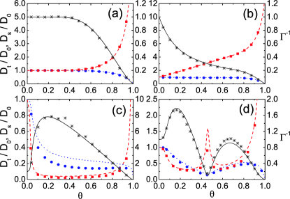
Figure 2: (Color online). $D_{s}/D_{0}$, $D_{t}/D_{0}$ and $\Gamma^{-1}$ as a function of loading $\theta=\langle n\rangle/n_{\mathrm{max}}$, $n_{\mathrm{max}}=13$; for (a) $\beta f(n)=0$, (b) $\beta f(n)=0.2n^{2}$, (c) $\beta f(n)=-0.2n^{2}$ and (d) $\beta f(n)$ that is subsequently concave, convex and again concave. The red dashed lines (analytical solution) and squares (simulations) show the transport diffusion and the blue dotted lines (analytical solution) and full circles (simulations) the self-diffusion (values on lhs axis). The analytical $\Gamma^{-1}$ (black full lines) are compared with the ratio of $D_{s}$ and $D_{t}$ (black stars) from the simulations (values on rhs axis).

For systems containing an arbitrary number of cavities, one has to take into account correlation effects. Finding an exact solution becomes difficult. Instead, we have performed kinetic Monte Carlo simulations (see supplementary material sup ). Our choice of rates is:

$$k_{nm}=\nu ne^{-\frac{\beta}{2}\left[f(n-1)+f(m+1)-f(n)-f(m)\right]}.$$ (16)

The factor $\nu$ determines the time scale. In the limit of infinite dilution, both $D_{t}$ and $D_{s}$ are equal to $\nu\lambda^{2}\equiv D_{0}$. For an ideal gas $f(n)=0$, $k_{nm}=\nu n$, i.e., the rates satisfy the law of mass action Van Kampen (1981). The simulations presented here are for 15 pairwise connected cavities, with $n_{\mathrm{max}}=13$. $D_{s}/D_{0}$, $D_{t}/D_{0}$ and $\Gamma^{-1}$ are plotted in Fig. 2 for different types of free energies, as a function of the loading $\theta=\langle n\rangle/n_{\mathrm{max}}$. Both the simulation data and the analytical curves Eqs. (11) and (14) are shown. The stars in the figures correspond to the ratio between the self- and transport diffusion obtained from simulations. Since correlations are included in the simulations but absent in the analytical result, the difference of the two curves is a measure of the effect of correlations on the diffusion. Figure 2(a) shows the diffusion for noninteracting particles $\beta f(n)=0$, with confinement (presence of $n_{\mathrm{max}}$). At low and medium loadings the particles are not influenced by the confinement; $\Gamma=1$ and $D_{s}=D_{t}$. At high loading, the confinement comes into play: $\Gamma^{-1}$ decreases, $D_{t}$ rises and $D_{s}$ lowers. The effect of correlations is negligible: the simulation data and analytical results coincide almost perfectly. Figure 2(b) shows the diffusion in the case of a convex free energy $\beta f(n)=0.2n^{2}$. $\Gamma^{-1}$ is lower than one, and $D_{t}$ is always larger than $D_{s}$. Correlations have a negligible influence. Fig. 2(c) shows the diffusion for a concave free energy $\beta f(n)=-0.2n^{2}$. As expected, $D_{s}>D_{t}$ for low to moderate loading. At moderate and high loading the “convexity effect” of confinement takes over: $\Gamma^{-1}$ decreases and eventually becomes smaller than one with $D_{t}>D_{s}$. This curve should be compared with Figs. $3(a),(c)$ in Chmelik et al. (2010). Noteworthy is the fact that the transport diffusion shows a minimum when the thermodynamic factor is around its maximum. This feature is in agreement with experimental observations Chmelik et al. (2010, 2009); Salles et al. (2010) and with MD simulations Krishna and van Baten (2011). It is now easily understood: when $\Gamma^{-1}$ is at its highest, the tendency to cluster is maximal, therefore the force opposing the current is also at its strongest. Turning to the effect of correlations, we note that they are quite strong: both $D_{t}$ and $D_{s}$ are significantly lower than the analytical results. The effect is the largest for self-diffusion. Nevertheless, the ratio of $D_{t}$ and $D_{s}$ is still very close to $\Gamma$, again in agreement with what is observed in experiments Chmelik et al. (2010) and MD simulations in similar systems Krishna and van Baten (2008). Fig. 2(d) shows the diffusion for a free energy that is first concave, then convex and then concave (see supplementary material sup for the exact form). For the first concave part the self-diffusion exceeds the transport diffusion. For the second concave part this is no longer the case, due to the confinement and the influence of the convex part in the middle. This is an illustration of how concavity is necessary but not sufficient for $D_{s}>D_{t}$. $D_{t}$ shows a (local) maximum in the convex part, whereas $D_{s}$ shows a (local) minimum. Correlations have noticeable effect, and are now more important for $D_{t}$ than for $D_{s}$. Notice that in all cases correlations lower the diffusion coefficients.

Motivated by the qualitative agreement with experiments, we have tried to reproduce the experimental results from Chmelik et al. (2010) quantitatively. Inspired by the form of the energy function for Lennard-Jones crystals Northby (1987), we take $\beta f(n)=an^{2}+bn^{3}$ for $n\leq n_{\mathrm{max}}$, with $n_{\mathrm{max}}=13$ taken from the experimental data Chmelik . The parameters $a$ and $b$ are determined by fitting the thermodynamic factor (Eq. (15)) with the experimental data, resulting in $\beta f(n)=0.000642n^{2}-0.0083n^{3}$. The parameters $\nu$ and $\lambda$ only appear in the combination $\nu\lambda^{2}$, which follows directly from the experimental value of $D_{t}$ at very low loading. In Fig. 3 we compare the obtained simulation results for $D_{s}$ and $D_{t}$ with experimental data of methanol in ZIF-8 Chmelik . Quantitative agreement is found for both $D_{s}$ and $D_{t}$ at all values of the loading. This is remarkable since $a$ and $b$ are determined from the equilibrium quantity $\Gamma$, and only the experimental value of $D_{t}$ at very low loading is used in the fit of $\nu\lambda^{2}$. A similar quantitative agreement is also found for ethanol in ZIF-8 (cf. supplementary material sup ).

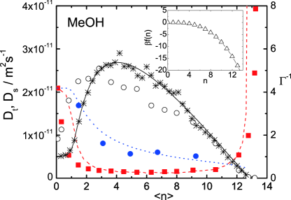
Figure 3: (Color online). Comparison of experimental data of methanol in ZIF-8 Chmelik with simulations from our model. The experimental self-diffusion and transport diffusion are represented by the blue full circles and red squares, respectively, with the corresponding results from simulations given by the blue dotted line and the red dashed line (values on lhs axis). The experimental (black open circles) and analytical (full black line) $\Gamma^{-1}$ are compared with the ratio of self- and transport diffusion (black stars) taken from the simulations (values on rhs axis). The inset shows $\beta f(n)$.

To conclude, we have introduced a model describing diffusion of interacting particles in discrete geometries. Exact analytical expressions for the self- and transport diffusion are given in the limiting case where correlations are absent, but are otherwise valid at all values of the concentration and for any interaction. We showed that the self-diffusion can exceed the transport diffusion when the free-energy function is concave as a function of the loading, resulting in the clustering of particles. By comparison with numerical simulations, the effect of the correlations is elucidated. Their influence is found to be significant for a free energy that is very concave or has several convex and concave sections. Nevertheless the ratio of self- and transport diffusion is always close to the thermodynamic factor, $D_{t}/D_{s}\approx\Gamma$, a result which is exact in the absence of correlations. Finally, we obtained quantitative agreement between numerical simulations of our model and experimental results of diffusion in ZIF-8 from Ref. Chmelik et al. (2010).