Fourier analysis of stationary time series in function space

Abstract

We develop the basic building blocks of a frequency domain framework for drawing statistical inferences on the second-order structure of a stationary sequence of functional data. The key element in such a context is the spectral density operator, which generalises the notion of a spectral density matrix to the functional setting, and characterises the second-order dynamics of the process. Our main tool is the functional Discrete Fourier Transform (fDFT). We derive an asymptotic Gaussian representation of the fDFT, thus allowing the transformation of the original collection of dependent random functions into a collection of approximately independent complex-valued Gaussian random functions. Our results are then employed in order to construct estimators of the spectral density operator based on smoothed versions of the periodogram kernel, the functional generalisation of the periodogram matrix. The consistency and asymptotic law of these estimators are studied in detail. As immediate consequences, we obtain central limit theorems for the mean and the long-run covariance operator of a stationary functional time series. Our results do not depend on structural modelling assumptions, but only functional versions of classical cumulant mixing conditions, and are shown to be stable under discrete observation of the individual curves.

T1Supported by a European Research Council Starting Grant Award.

and

1 Introduction

In the usual context of functional data analysis, one wishes to make inferences pertaining to the law of a continuous time stochastic process $\{X(\tau);\tau\in[0,1]\}$ on the basis of a collection of $T$ realisations of this stochastic process, $\{X_{t}(\tau)\}_{t=0}^{T-1}$. These are modelled as random elements of the separable Hilbert space $L^{2}([0,1],\mathbb{R})$ of square integrable real functions defined on $[0,1]$. Statistical analyses typically focus on the first and second-order characteristics of this law [see, e.g., Grenander (1981), Rice and Silverman (1991), Ramsay and Silverman (2005)] and are, for the most part, based on the fundamental Karhunen–Loève decomposition [Karhunen (1947), Lévy (1948), Dauxois, Pousse and Romain (1982), Hall and Hosseini-Nasab (2006)]. Especially the second-order structure of random functions is central to the analysis of functional data, as it is connected with the smoothness properties of the random functions and their optimal finite-dimensional representations [e.g., Adler (1990)]. When functional data are independent and identically distributed, the entire second-order structure is captured by the covariance operator [Grenander (1981)], or related operators [e.g., Locantore et al. (1999), Kraus and Panaretos (2012)]. The assumption of identical distribution can be relaxed, and this is often done by allowing a varying first-order structure through the inclusion of covariate variables (or functions) in the context of functional regression and analysis of variance models; see Cuevas, Febrero and Fraiman (2002); Cardot and Sarda (2006); Yao, Müller and Wang (2005). Second-order structure has been studied in the “nonidentically distributed” context mostly in terms of the so-called common principal components model [e.g., Benko, Härdle and Kneip (2009)], in a comparison setting, where two functional populations are compared with respect to their covariance structure [e.g., Panaretos, Kraus and Maddocks (2010), Boente, Rodriguez and Sued (2011), Horváth and Kokoszka (2012), Fremdt et al. (2013)], and in the context of detection of sequential changes in the covariance structure of functional observations [Horváth, Hušková and Kokoszka (2010)]; see Horváth and Kokoszka (2012) for an overview.

For sequences of potentially dependent functional data, Gabrys and Kokoszka (2007) and Gabrys, Horváth and Kokoszka (2010) study the detection of correlation. To obtain a complete description of the second-order structure of dependent functional sequences, one needs to consider autocovariance operators relating different lags of the series, as is the case in multivariate time series. This study will usually be carried out under the assumption of stationarity. Research in this context has mostly focused on stationary functional series that are linear. Problems considered include that of the estimation of the second-order structure [e.g., Mas (2000), Bosq (2002), Dehling and Sharipov (2005)] and that of prediction [e.g., Antoniadis and Sapatinas (2003), Ferraty and Vieu (2004), Antoniadis, Paparoditis and Sapatinas (2006)]. It can be said that the linear case is now relatively well understood, and Bosq (2000) and Bosq and Blanke (2007) provide a detailed overview thereof.

Recent work has attempted to move functional time series beyond linear models and construct inferential procedures for time series that are not a priori assumed to be described by a particular model, but are only assumed to satisfy certain weak dependence conditions. Hörmann and Kokoszka (2010) consider the effect that weak dependence can have on the principal component analysis of functional data and propose weak dependence conditions under which they study the stability of procedures that assume independence. They also study the problem of inferring the long-run covariance operator by means of finite-dimensional projections. Horváth, Kokoszka and Reeder (2013) give a central limit theorem for the mean of a stationary weakly dependent functional sequence, and propose a consistent estimator for the long-run covariance operator.

In this paper, rather than focus on isolated characteristics such as the long-run covariance, we consider the problem of inferring the complete second-order structure of stationary functional time series without any structural modelling assumptions, except for cumulant-type mixing conditions. Our approach is to study the problem via Fourier analysis, formulating a frequency domain framework for weakly dependent functional data. To this aim, we employ suitable generalisations of finite-dimensional notions [e.g., Brillinger (2001), Bloomfield (2000), Priestley (2001)] and provide conditions for these to be well defined.

We encode the complete second-order structure via the spectral density operator, the Fourier transform of the collection of autocovariance operators, seen as operator-valued functions of the lag argument; see Proposition 2.1. We propose strongly consistent and asymptotically Gaussian estimators of the spectral density operator based on smoothing the periodogram operator—the functional analogue of the periodogram matrix; see Theorems 3.6 and 3.7. In this sense, our methods can be seen as functional smoothing, as overviewed in Ferraty and Vieu (2006), but in an operator context; see also, for example, Ferraty et al. (2011a), Ferraty et al. (2011b), Laib and Louani (2010). As a by-product, we also obtain central limit theorems for both the mean and long-run covariance operator of stationary time series paralleling or extending the results of Horváth, Kokoszka and Reeder (2013), but under different weak dependence conditions; see Corollaries 2.4 and 3.8. The key result employed in our analysis is the asymptotic representation of the discrete Fourier transform of a weakly dependent stationary functional process as a collection of independent Gaussian elements of $L^{2}([0,1],\mathbb{C})$, the Hilbert space of square integrable complex-valued functions, with mean zero and covariance operator proportional to the spectral density operator at the corresponding frequency (Theorem 2.2). Weak dependence conditions required to yield these results are moment type conditions based on cumulant kernels, which are functional versions of cumulant functions. A noteworthy feature of our results and methodology is that they do not require the projection onto a finite-dimensional subspace, as is often the case with functional time series [Hörmann and Kokoszka (2010), Sen and Klüppelberg (2010)]. Rather, our asymptotic results hold for purely infinite-dimensional functional data.

The paper is organised in seven sections and the supplementary material [Panaretos and Tavakoli (2013)]. The building blocks of the frequency domain framework are developed in Section 2. After some basic definitions and introduction of notation, Section 2.1 provides conditions for the definition of the spectral density operator. The functional version of the discrete Fourier transform is introduced in Section 2.2, where its analytical and asymptotic properties are investigated. Section 2.3 then introduces the periodogram operator and studies its mean and covariance structure. The estimation of the spectral density operator by means of smoothing is considered in Section 3. Section 4 provides a detailed discussion on the weak dependence conditions introduced in earlier sections. The effect of observing only discretely sampled functions is considered in Section 5, where the consistency is seen to persist under conditions on the nature of the discrete sampling scheme. Finite-sample properties are illustrated via simulation in Section 6. Technical background and several lemmas required for the proofs or the main results are provided in a an extensive supplementary material [Panaretos and Tavakoli (2013)]. One of our technical results, Lemma 7.1, collects some results that may be of independent interest in functional data analysis when seeking to establish tightness in order to extend finite-dimensional convergence results to infinite dimensions; it is given in the main paper, in a short section (Section 7).

2 Spectral characteristics of stationary functional data

We start out this section with an introduction of some basic definitions and notation. Let $\{X_{t}\}_{t\in\mathbb{Z}}$ be a functional time series indexed by the integers, interpreted as time. That is, for each $t$, we understand $X_{t}$ as being a random element of $L^{2}([0,1],\mathbb{R})$, with

$$\tau\mapsto X_{t}(\tau)\in\mathbb{R},\qquad\tau\in[0,1],$$

denoting its parametrisation. Though all our results will be valid for any separable Hilbert space, we choose to concentrate on $L^{2}([0,1],\mathbb{R})$, as this is the paradigm for functional data analysis. We denote the inner product in $L^{2}([0,1],\mathbb{R})$ by $\langle\cdot,\cdot\rangle$, and the induced norm by $\|\cdot\|_{2}$,

$$\langle f,g\rangle=\biggl{(}\int_{0}^{1}f(\tau)g(\tau)\,{d}\tau\biggr{)}^{1/2},\qquad\|g\|_{2}=\langle g,g\rangle^{1/2},\qquad f,g\in L^{2}\bigl{(}[0,1],\mathbb{R}\bigr{)}.$$

Equality of $L^{2}$ elements will be understood in the sense of the norm of their difference being zero. The imaginary number will de denoted by $\mathrm{i}$, $\mathrm{i}^{2}=-1$, and the complex conjugate of $z\in\mathbb{C}$ will be denoted as $\bar{z}$. We also denote $\Delta^{(T)}(\omega)=\sum_{t=0}^{T-1}\exp(-\mathrm{i}\omega t).$ The Hermitian adjoint of an operator $\mathscr{A}$ will be denoted as $\mathscr{A}^{{\dagger}}$. For a function $g\dvtx D\subset\mathbb{R}^{n}\rightarrow\mathbb{C},$ we denote $\|g\|_{\infty}=\sup_{{\mathbf{x}}\in D}|g({\mathbf{x}})|.$

Throughout, we assume that the series $\{X_{t}\}_{t\in\mathbb{Z}}$ is strictly stationary: for any finite set of indices $I\subset\mathbb{Z}$ and any $s\in\mathbb{Z}$, the joint law of $\{X_{t},t\in I\}$ coincides with that of $\{X_{t+s},t\in I\}$. If $\mathbb{E}\|X_{0}\|_{2}<\infty,$ the mean of $X_{t}$ is well defined, belongs to $L^{2}([0,1],\mathbb{R})$, and is independent of $t$ by stationarity, $\mu(\tau)=\mathbb{E}X_{t}(\tau).$ We also define the autocovariance kernel at lag $t$ by

$$\mathpzc{r}_{t}(\tau,\sigma)=\mathbb{E}\bigl{[}\bigl{(}X_{t+s}(\tau)-\mu(\tau)\bigr{)}\bigl{(}X_{s}(\sigma)-\mu(\sigma)\bigr{)}\bigr{]},\qquad\tau,\sigma\in[0,1]\mbox{ and }t,s\in\mathbb{Z}.$$

This kernel is well defined in the $L^{2}$ sense if $\mathbb{E}\|X_{0}\|^{2}_{2}<\infty$; if continuity in mean square of $X_{t}$ is assumed, then it is also well defined pointwise. Each kernel $\mathpzc{r}_{t}$ induces a corresponding operator $\mathscr{R}_{t}\dvtx L^{2}([0,1],\mathbb{R})\rightarrow L^{2}([0,1],\mathbb{R})$ by right integration, the autocovariance operator at lag $t$,

$$\mathscr{R}_{t}h(\tau)=\int_{0}^{1}\mathpzc{r}_{t}(\tau,\sigma)h(\sigma)\,{d}\sigma=\operatorname{cov}\bigl{[}\bigl{\langle}X_{0},h\rangle,X_{t}(\tau)\bigr{]},\qquad h\in L^{2}\bigl{(}[0,1],\mathbb{R}\bigr{)}.$$

One of the notions we will employ to quantify the weak dependence among the observations $\{X_{t}\}$ is that of a cumulant kernel of the series; the pointwise definition of a $k$th order cumulant kernel is

$$\operatorname{cum}\bigl{(}X_{t_{1}}(\tau_{1}),\ldots,X_{t_{k}}(\tau_{k})\bigr{)}=\sum_{\nu=(\nu_{1},\ldots,\nu_{p})}(-1)^{p-1}(p-1)!\prod_{l=1}^{p}\mathbb{E}\biggl{[}\prod_{j\in\nu_{l}}X_{t_{j}}(\tau_{j})\biggr{]},$$

where the sum extends over all unordered partitions of $\{1,\ldots,k\}$. Assuming $\mathbb{E}\|X_{0}\|_{2}^{l}<\infty$ for $l\geq 1$ guarantees that the cumulant kernels are well defined in an $L^{2}$ sense. A cumulant kernel of order $2k$ gives rise to a corresponding $2k$th order cumulant operator $\mathscr{R}_{t_{1},\ldots,t_{2k-1}}\dvtx L^{2}([0,1]^{k},\mathbb{R})\rightarrow L^{2}([0,1]^{k},\mathbb{R})$, defined by right integration,

$$\mathscr{R}_{t_{1},\ldots,t_{2k-1}}h(\tau_{1},\ldots,\tau_{k})$$

$$\qquad=\int_{[0,1]^{k}}\operatorname{cum}\bigl{(}X_{t_{1}}(\tau_{1}),\ldots,X_{t_{2k-1}}(\tau_{2k-1}),X_{0}(\tau_{2k})\bigr{)}$$

$$\hskip 59.0pt{}\times h(\tau_{k+1},\ldots,\tau_{2k})\,{d}\tau_{k+1}\cdots\,{d}\tau_{2k}.$$

2.1 The spectral density operator

The autocovariance operators encode all the second-order dynamical properties of the series and are typically the main focus of functional time series analysis. Since we wish to formulate a framework for a frequency domain analysis of the series $\{X_{t}\}$, we need to consider a suitable notion of Fourier transform of these operators. This we call the spectral density operator of $\{X_{t}\}$, defined rigorously in Proposition 2.1 below. Results of a similar flavour related to Fourier transforms between general Hilbert spaces can be traced back to, for example, Kolmogorov (1978); we give here the precise versions that we will be requiring, for completeness, since those results do not readily apply in our setting.

Proposition 2.1.

Suppose $p=2$ or $p=\infty,$ and consider the following conditions:

I($p$) the autocovariance kernels satisfy $\sum_{t\in\mathbb{Z}}\|\mathpzc{r}_{t}\|_{p}<\infty;$

II the autocovariance operators satisfy $\sum_{t\in\mathbb{Z}}|\!|\!|\mathscr{R}_{t}|\!|\!|_{1}<\infty,$ where $|\!|\!|\mathscr{R}_{t}|\!|\!|_{1}$ is the nuclear norm or Schatten 1-norm; see Paragraph F.1.1 in the supplementary material [Panaretos and Tavakoli (2013)]. Then, under I($p$), for any $\omega\in\mathbb{R}$, the following series converges in $\|\cdot\|_{p}$:

$$\mathpzc{f}_{\omega}(\cdot,\cdot)=\frac{1}{2\pi}\sum_{t\in\mathbb{Z}}\exp(-\mathrm{i}\omega t)\mathpzc{r}_{t}(\cdot,\cdot).$$ (1)

We call the limiting kernel $\mathpzc{f}_{\omega}$ the spectral density kernel at frequency $\omega$. It is uniformly bounded and also uniformly continuous in $\omega$ with respect to $\|\cdot\|_{p}$; that is, given $\varepsilon>0$, there exists a $\delta>0$ such that

$$|\omega_{1}-\omega_{2}|<\delta\quad\Longrightarrow\quad\|\mathpzc{f}_{\omega_{1}}-\mathpzc{f}_{\omega_{2}}\|_{p}<\varepsilon.$$

The spectral density operator $\mathscr{F}_{\omega}$, the operator induced by the spectral density kernel through right-integration, is self-adjoint and nonnegative definite for all $\omega\in\mathbb{R}$. Furthermore, the following inversion formula holds in $\|\cdot\|_{p}$:

$$\int_{0}^{2\pi}\mathpzc{f}_{\alpha}(\tau,\sigma)e^{\mathrm{i}t\alpha}\,{d}\alpha=\mathpzc{r}_{t}(\tau,\sigma)\qquad\forall t,\tau,\sigma.$$ (2)

Under only II, we have

$$\mathscr{F}_{\omega}=\frac{1}{2\pi}\sum_{t\in\mathbb{Z}}e^{-\mathrm{i}\omega t}\mathscr{R}_{t},$$ (3)

where the convergence holds in nuclear norm. In particular, the spectral density operators are nuclear, and $|\!|\!|\mathscr{F}_{\omega}|\!|\!|_{1}\leq\frac{1}{2\pi}\sum_{t}|\!|\!|\mathscr{R}_{t}|\!|\!|_{1}<\infty.$

See Proposition A.1 in the supplementary material [Panaretos and Tavakoli (2013)].

The inversion relationship (2), in particular, shows that the autocovariance operators and the spectral density operators comprise a Fourier pair, thus reducing the study of second-order dynamics to that of the study of the spectral density operator.

We use the term spectral density operator by analogy to the multivariate case, in which the Fourier transform of the autocovariance functions is called the spectral density matrix; see, for example, Brillinger (2001). In our case, since the time series takes values in $L^{2}([0,1],\mathbb{R})$, the autocovariance functions are in fact operators and their Fourier transform is an operator, hence the term spectral density operator. In light of the inversion formula (2), for fixed $(\tau,\sigma),$ we can think of the $\omega\mapsto\mathpzc{f}_{\omega}(\tau,\sigma)$ as being a (complex) measure, giving the distribution of energy between $X_{t}(\tau)$ and $X_{0}(\sigma)$ across different frequencies. That is, $\omega\mapsto\mathpzc{f}_{\omega}(\tau,\tau)\geq 0$ gives the power spectrum of the univariate time series $\{X_{t}(\tau)\}_{t\in\mathbb{Z}}$, while given $\tau\neq\sigma$, $\omega\mapsto\mathpzc{f}_{\omega}(\tau,\sigma)\in\mathbb{C}$ gives the cross spectrum of the univariate time series $\{X_{t}(\tau)\}_{t\in\mathbb{Z}}$ with $\{X_{t}(\sigma)\}_{t\in\mathbb{Z}}$. When a point-wise interpretation of $\{X_{t}\}_{t\in\mathbb{Z}}$ is not possible (e.g., because it is only interpretable via $L^{2}$ equivalence classes), the spectral density operator admits a weak interpretation as follows: given $L^{2}$ elements $\psi\neq\phi$, the mapping $\omega\mapsto\langle\psi,\mathscr{F}_{\omega}\psi\rangle\geq 0$ is the power spectrum of the univariate time series $\{\langle\psi,X_{t}\rangle\}_{t\in\mathbb{Z}}$, while $\omega\mapsto\langle\psi,\mathscr{F}_{\omega}\phi\rangle=\langle\mathscr{F}_{\omega}\psi,\phi\rangle\in\mathbb{C}$ is the cross spectrum of the univariate time series $\{\langle\psi,X_{t}\rangle\}_{t\in\mathbb{Z}}$ with the univariate time series $\{\langle\phi,X_{t}\rangle\}_{t\in\mathbb{Z}}$. In this sense, $\mathscr{F}_{\omega}$ provides a complete characterisation of the second-order dynamics of the functional process $\{X_{t}\}$; see also Panaretos and Tavakoli (2013) for the role of the spectral density operator in the spectral representation and the harmonic principal component analysis of functional time series.

2.2 The functional discrete Fourier transform and its properties

In practice, a stretch of length $T$ of the series $\{X_{t}\}_{t\in\mathbb{Z}}$ will be available, and we will wish to draw inferences on the spectral density operator based on this finite stretch. The main tool that we will employ is the functional version of the discrete Fourier transform (DFT). In particular, define the functional Discrete Fourier Transform (fDFT) of $\{X_{t}\}_{t=0}^{T-1}$ to be

$$\widetilde{X}_{\omega}^{(T)}(\tau)=(2\pi T)^{-1/2}\sum_{t=0}^{T-1}X_{t}(\tau)\exp(-\mathrm{i}\omega t).$$

It is of interest to note here that the construction of the fDFT does not require the representation of the data in a particular basis. The fDFT transforms the $T$ functional observations to a mapping from $\mathbb{R}$ into $L^{2}([0,1],\mathbb{C})$. It straightforwardly inherits some basic analytical properties that its finite-dimensional counterpart satisfies; for example, it is $2\pi$-periodic and Hermitian with respect to $\omega$, and linear with respect to the series $\{X_{t}\}$.

The extension of the stochastic properties of the multivariate DFT to the fDFT, however, is not as straightforward. It is immediate that $\mathbb{E}\|\widetilde{X}_{\omega}^{(T)}\|_{2}^{l}<~{}\infty$ if $\mathbb{E}\|X_{t}\|_{2}^{l}<\infty$, and hence the fDFT is almost surely in $L^{2}([0,1],\mathbb{C})$ if $\mathbb{E}\|X_{t}\|_{2}^{2}<\infty$. We will see that the asymptotic covariance operator of this object coincides with the spectral density operator. Most importantly, we prove below that the fundamental stochastic property of the multivariate DFT can be adapted and extended to the infinite-dimensional case; that is, under suitable weak dependence conditions, as $T\rightarrow\infty$, the fDFT evaluated at distinct frequencies yields independent and Gaussian random elements of $L^{2}([0,1],\mathbb{C})$. The important aspect of this limit theorem is that it does not require the assumption of any particular model for the stationary series, and imposes only cumulant mixing conditions. A more detailed discussion of these conditions is provided in Section 4.

Theorem 2.2 ((Asymptotic distribution of the fDFT))

Let $\{X_{t}\}_{t=0}^{T-1}$ be a strictly stationary sequence of random elements of $L^{2}([0,1],\mathbb{R})$, of length $T$. Assume the following conditions hold:

$\mathbb{E}\|X_{0}\|_{2}^{k}<\infty$, $\sum_{t_{1},\ldots,t_{k-1}=-\infty}^{\infty}\|\operatorname{cum}(X_{t_{1}},\ldots,X_{t_{k-1}},X_{0})\|_{2}<\infty,\break\forall k\geq 2$.

$\sum_{t\in\mathbb{Z}}|\!|\!|\mathscr{R}_{t}|\!|\!|_{1}<\infty.$

Then, for $\omega_{1,T}:=\omega_{1}=0,$ $\omega_{2,T}:=\omega_{2}=\pi,$ and distinct integers

$$s_{3,T},\ldots,s_{J,T}\in\bigl{\{}1,\ldots,\bigl{\lfloor}(T-1)/2\bigr{\rfloor}\bigr{\}}$$

such that

$$\omega_{j,T}:=\frac{2\pi s_{j,T}}{T}\stackrel{{\scriptstyle T\rightarrow\infty}}{{\longrightarrow}}\omega_{j},\qquad j=3,\ldots,J,$$

we have

$$\widetilde{X}_{\omega_{1}}^{(T)}-\sqrt{\frac{T}{2\pi}}\mu\stackrel{{\scriptstyle d}}{{\longrightarrow}}\widetilde{X}_{\omega_{1}}\qquad\mbox{as }T\rightarrow\infty,$$ (4)

and $\widetilde{X}_{\omega_{j,T}}^{(T)}\stackrel{{\scriptstyle d}}{{\longrightarrow}}\widetilde{X}_{\omega_{j}},\mbox{as }T\rightarrow\infty,j=2,\ldots,J$ where $\{\widetilde{X}_{\omega_{j}}\}$ are independent mean zero Gaussian elements of $L^{2}([0,1],\mathbb{R})$ for $j=1,2$, and of $L^{2}([0,1],\mathbb{C})$ for $j=3,\ldots,J,$ with covariance operators $\mathscr{F}_{\omega_{j}}$, respectively.

Remark 2.3.

Though the $\{\omega_{j,T}\}_{j=3}^{J}$ are distinct for every $T$, the limiting frequencies $\{\omega_{j}\dvtx j=3,\ldots,J\}$ need not be distinct.

Note here that condition (i) with $k=2$ is already required in order to define the spectral density kernel and operator in Proposition 2.1. Condition (i) for $k\geq 3$ is the generalisation of the standard multivariate cumulant condition to the functional case [Brillinger (2001), Condition 2.6.1], and reduces to that exact same condition if the data are finite-dimensional. Condition (ii) is required so that the spectral density operator be a nuclear operator at each $\omega$ [which is in turn a necessary condition for the weak limit of the fDFT to be almost surely in $L^{2}([0,1],\mathbb{C})$]. As we shall see, condition (ii) is, in fact, a sufficient condition for tightness of the fDFT, seen as a functional process indexed by frequency.

Proof of Theorem 2.2 Consider $p_{\omega}^{(T)}(\tau,\sigma)=\widetilde{X}_{\omega}^{(T)}(\tau)\widetilde{X}_{-\omega}^{(T)}(\sigma),$ and assume initially that $\mu=0$. We will treat the case $\mu\neq 0$ at the end of the proof. First we show that for any $\omega$ (or sequence $\omega_{T}$), the sequence of random elements $\widetilde{X}_{\omega}^{(T)},T=1,2,\ldots,$ is tight. To do this, we shall use Lemma 7.1. Fix an orthonormal basis $\{\varphi_{n}\}_{n\geq 1}$ of $L^{2}([0,1],\mathbb{R})$ and let $H=L^{2}([0,1],\mathbb{C})$. We notice that $p^{(T)}_{\omega}$ is a random element of the (complete) tensor product space $H\otimes H$, with scalar product and norm ${\langle\cdot,\cdot\rangle}_{H\otimes H},\|\cdot\|_{H\otimes H}$, respectively; see Weidmann [(1980), Paragraph 3.4], for instance. Notice that $|{\langle\widetilde{X}_{\omega},\varphi_{n}\rangle}|^{2}={\langle p_{\omega}^{(T)},\varphi_{n}\otimes\varphi_{n}\rangle}.$ Since $\mathbb{E}\|p_{\omega}^{(T)}\|_{H\otimes H}<\infty$ and the projection $\mathcal{P}_{n}\dvtx H\otimes H\rightarrow\mathbb{C}$ defined by $\mathcal{P}_{n}(f)={\langle f,\varphi_{n}\otimes\varphi_{n}\rangle}_{H\otimes H}$ is continuous and linear, we deduce

$$\mathbb{E}\bigl{|}\bigl{\langle}\widetilde{X}_{\omega}^{(T)},\varphi_{n}\bigr{\rangle}\bigr{|}^{2} = \mathbb{E}\mathcal{P}_{n}p_{\omega}^{(T)}=\mathcal{P}_{n}\mathbb{E}p_{\omega}^{(T)}=\frac{1}{2\pi}\mathcal{P}_{n}\int_{-\pi}^{\pi}F_{T}(\omega-\alpha)\mathpzc{f}_{\alpha}\,d\alpha$$

$$= \frac{1}{2\pi}\int_{-\pi}^{\pi}F_{T}(\omega-\alpha)\mathcal{P}_{n}\mathpzc{f}_{\alpha}\,d\alpha\leq\sup_{\alpha\in\mathbb{R}}|\mathcal{P}_{n}\mathpzc{f}_{\alpha}|.$$

The third equality comes from Proposition 2.5 (which is independent of previous results), the fourth equality follows from Tonelli’s theorem [Wheeden and Zygmund (1977), page 92], and the last inequality is Young’s inequality [Hunter and Nachtergaele (2001), Theorem 12.58]. Notice that $|\mathcal{P}_{n}\mathpzc{f}_{\alpha}|=|{\langle\mathscr{F}_{\alpha}\varphi_{n},\varphi_{n}\rangle}|\leq\sum_{t}|{\langle\mathscr{R}_{t}\varphi_{n},\varphi_{n}\rangle}|$ by (3). Setting $a_{n}=\sum_{t}|{\langle\mathscr{R}_{t}\varphi_{n},\varphi_{n}\rangle}|$, which is independent of $\alpha$ and $T$, we have $\mathbb{E}|{\langle\widetilde{X}_{\omega}^{(T)},\varphi_{n}\rangle}|^{2}\leq a_{n},$ and $\sum_{n}a_{n}\leq\sum_{t\in\mathbb{Z}}|\!|\!|\mathscr{R}_{t}|\!|\!|_{1}<\infty.$ Therefore, we have proven that $\widetilde{X}_{\omega}^{(T)}$ is tight. Consequently, the random element $(\widetilde{X}_{\omega_{1,T}}^{(T)},\ldots,\widetilde{X}_{\omega_{J,T}}^{(T)})$ of $(L^{2}([0,1],\mathbb{C}))^{J}$ is also tight. Its asymptotic distribution is therefore determined by the convergence of its finite-dimensional distributions; see, for example, Ledoux and Talagrand [(1991), Paragraph 2.1]. Thus, to complete the proof, it suffices to show that for any $\psi_{1},\ldots,\psi_{J}\in L^{2}([0,1],\mathbb{C})$,

$$\bigl{(}\bigl{\langle}\widetilde{X}_{\omega_{1,T}}^{(T)},\psi_{1}\bigr{\rangle},\ldots,\bigl{\langle}\widetilde{X}_{\omega_{J,T}}^{(T)},\psi_{J}\bigr{\rangle}\bigr{)}\stackrel{{\scriptstyle d}}{{\longrightarrow}}\bigl{(}\langle\widetilde{X}_{\omega_{1}},\psi_{1}\rangle,\ldots,\langle\widetilde{X}_{\omega_{J}},\psi_{J}\rangle\bigr{)},$$ (5)

where $\widetilde{X}_{\omega_{j}}\sim{\mathcal{N}(0,\mathscr{F}_{\omega_{j}})}$ are independent Gaussian random elements of $H$, where $H=L^{2}([0,1],\mathbb{R})$ if $j=1,2$ and $H=L^{2}([0,1],\mathbb{C})$ if $j=3,\ldots,J$. This is a consequence of the following claim, which is justified by Brillinger [(2001), Theorem 4.4.1]:

[(I)]

For $j=1,\ldots,J$, let $\psi_{j}=\varphi_{2j-1}+\mathrm{i}\varphi_{2j}$, where $\varphi_{1},\ldots,\varphi_{2J}\in L^{2}([0,1],\mathbb{R})$, and ${\mathbf{Y}}_{t}=(Y_{t}(1),\ldots,Y_{t}(2J))\in\mathbb{R}^{2J}$ be the vector time series with coordinates $Y_{t}(l)={\langle X_{t},\varphi_{l}\rangle}.$ Then $\widetilde{{\mathbf{Y}}}_{\omega_{j,T}}^{(T)}\stackrel{{\scriptstyle d}}{{\rightarrow}}\widetilde{{\mathbf{Y}}}_{\omega_{j}}$, where $\{\widetilde{{\mathbf{Y}}}_{\omega_{j}}\}$ are independent mean zero complex Gaussian random vectors with covariance matrix ${\mathbf{F}}_{\omega_{j}},$ $({\mathbf{F}}_{\omega_{j}})_{sl}:=F_{\omega_{j}}(s,l)={\langle\mathscr{F}_{\omega_{j}}\varphi_{l},\varphi_{s}\rangle}.$

For the case $\mu\neq 0$, we only need to consider $j=1,2$ since $\widetilde{(X-\mu)}_{\omega_{j,T}}^{(T)}=\widetilde{X}_{\omega_{j,T}}^{(T)}$ for $j=3,\ldots,J$. We need to show that

$$\widetilde{X}_{\omega_{1}}^{(T)}-\sqrt{\frac{T}{2\pi}}\mu=(2\pi T)^{-1/2}\sum_{t=0}^{T-1}(X_{t}-\mu)\stackrel{{\scriptstyle d}}{{\rightarrow}}\widetilde{X}_{0},$$ (6)

and also that

$$\widetilde{X}_{\omega_{2}}^{(T)}=(2\pi T)^{-1/2}\sum_{t=0}^{T-1}(-1)^{t}X_{t}\stackrel{{\scriptstyle d}}{{\rightarrow}}\widetilde{X}_{\pi}.$$ (7)

The weak convergence in (6) follows immediately from the case $\mu=0$. For (7), notice that

$$\widetilde{X}_{\omega_{2}}^{(T)}=(2\pi T)^{-1/2}\sum_{t=0}^{T-1}(-1)^{t}(X_{t}-\mu)+\mu(2\pi T)^{-1/2}\sum_{t=0}^{T-1}(-1)^{t}.$$

The first summand is the discrete Fourier transform of a zero mean random process, and converges to $\widetilde{X}_{\omega_{2}}$. The second summand is deterministic and bounded by $\|\mu\|(2\pi T)^{-1/2}$, which tends to zero. Finally, the continuous mapping theorem for metric spaces [Pollard (1984)] yields (7).

The theorem has important consequences for the statistical analysis of a functional time series. It essentially allows us to transform a collection of weakly dependent functional data of an unknown distribution, to a collection of approximately independent and Gaussian functional data. In particular, let $\{\omega_{j,T}\}_{j=1}^{J}$ be $J$ sequences (in $T$) of frequencies, such that $\omega_{j,T}\stackrel{{\scriptstyle T\rightarrow\infty}}{{\longrightarrow}}\omega\neq 0$, for all $1\leq j\leq J$. Then, provided $T$ is large enough, $\{\widetilde{X}_{\omega_{j,T}}^{(T)}\}_{j=1}^{J}$ is a collection of $J$ approximately i.i.d. mean zero complex Gaussian random functions with covariance operator $\mathscr{F}_{\omega}$. The size $J$ of the sample is not allowed to grow with $T$, however. From a practical point of view, it can be chosen to be large, provided that the $\omega_{j,T}$ are not too far from $\omega$. We will make heavy use of this result in order to construct consistent and asymptotically Gaussian estimators of the spectral density operator by means of the periodogram kernel, defined in the next section.

We also remark that the weak convergence relation in equation (4) can be re-expressed to trivially yield the corollary:

Corollary 2.4 ((Central limit theorem for cumulant mixing functional series)).

Let $\{X_{t}\}_{t=0}^{T}$ be a strictly stationary sequence of random elements of $L^{2}([0,1],\mathbb{R})$ of length $T$ satisfying conditions (i) and (ii) of Theorem 2.2. Then

$$\sqrt{T}\Biggl{(}\frac{1}{T}\sum_{t=0}^{T-1}X_{t}(\tau)-\mu(\tau)\Biggr{)}\stackrel{{\scriptstyle d}}{{\longrightarrow}}\mathcal{N}\biggl{(}0,\sum_{t\in\mathbb{Z}}\mathscr{R}_{t}\biggr{)}.$$

This provides one of the first instances of central limit theorems for functional series under no structural modelling assumptions beyond weak dependence. To our knowledge, the only other similar result is given in recent work by Horváth, Kokoszka and Reeder (2013), who obtain the same limit under different weak dependence conditions, namely $L^{p}$-$m$-approximability.

The covariance operator of the limiting Gaussian measure is the functional analogue of the long-run covariance matrix from multivariate time series. We will revisit this operator in Section 3, where we will derive a related central limit theorem.

2.3 The periodogram kernel and its properties

The covariance structure of the weak limit of the fDFT given in Theorem 2.2 motivates the consideration of the empirical covariance of the functional DFT as a basis for the estimation of the spectral density operator. Thus, as with the multivariate case, we are led to consider tensor products of the fDFT leading to the notion of a periodogram kernel. Define the periodogram kernel as

$$p_{\omega}^{(T)}(\tau,\sigma)=\bigl{[}\widetilde{X}_{\omega}^{(T)}(\tau)\bigr{]}\bigl{[}\widetilde{X}_{\omega}^{(T)}(\sigma)\bigr{]}^{{\dagger}}=\widetilde{X}_{\omega}^{(T)}(\tau)\widetilde{X}_{-\omega}^{(T)}(\sigma).$$

If we slightly abuse notation and also write $\|\cdot\|_{2}$ for the norm in $L^{2}([0,1]^{2},\mathbb{C})$, we have $\|p_{\omega}^{(T)}\|_{2}=\|\widetilde{X}_{\omega}^{(T)}\|^{2}_{2},$ and hence $\mathbb{E}\|p_{\omega}^{(T)}\|^{l}_{2}<\infty$, if $\mathbb{E}\|X_{t}\|_{2}^{2l}<\infty$. The expectation of the periodogram kernel is thus well defined, and, letting $a_{T}=\sum_{t=-T}^{T}e^{-\mathrm{i}\omega t}\mathpzc{r}_{t}$, Lemma F.3 yields $\mathbb{E}p_{\omega}^{(T)}=T^{-1}(a_{0}+a_{1}+\cdots+a_{T-1}).$ That is, the expectation of the periodogram kernel is a Cesàro-sum of the partial sums of the series defining the spectral density kernel. Therefore, in order to probe the properties of the periodogram kernel, we can make use of the Fejér kernel

$$F_{T}(\omega)=\frac{1}{T}\biggl{(}\frac{\sin(T\omega/2)}{\sin(\omega/2)}\biggr{)}^{2}=\frac{1}{T}\bigl{|}\Delta^{(T)}(\omega)\bigr{|}^{2}.$$

It will thus be useful to recall some properties of $F_{T}$: $\int_{-\pi}^{\pi}F_{T}=2\pi,F_{T}(0)=T,F_{T}(\omega)\sim O(T)$ uniformly in $\omega$, and $F_{T}(2\pi s/T)=0$ for $s$ an integer with $s\not\equiv 0\,\mathrm{mod}\,T.$ This last property will be used often. We will also be making use of the following cumulant mixing condition, defined for fixed $l\geq 0$ and $k=2,3,\ldots.$

Condition $\mathrm{C}(l,k)$.

For each $j=1,\ldots,k-1,$

$$\sum_{t_{1},\ldots,t_{k-1}=-\infty}^{\infty}\bigl{(}1+|t_{j}|^{l}\bigr{)}\bigl{\|}\operatorname{cum}(X_{t_{1}},\ldots,X_{t_{k-1}},X_{0})\bigr{\|}_{2}<\infty.$$

With this definition in place, we may determine the exact mean of the periodogram kernel:

Proposition 2.5.

Assuming that $\mathrm{C}(0,2)$ holds true, we have, for each $\omega\in\mathbb{R},$

$$\mathbb{E}\bigl{[}p_{\omega}^{(T)}(\tau,\sigma)\bigr{]}=\frac{1}{2\pi}\int_{-\pi}^{\pi}F_{T}(\omega-\alpha)\mathpzc{f}_{\alpha}(\tau,\sigma)\,d\alpha+\frac{1}{2\pi}\mu(\tau)\mu(\sigma)F_{T}(\omega)\qquad\mbox{in }L^{2}.$$

In particular, if $\omega=2\pi s/T,$ with $s$ an integer such that $s\not\equiv 0\,\mathrm{mod}\,T,$

$$\mathbb{E}\bigl{[}p_{\omega}^{(T)}(\tau,\sigma)\bigr{]}=\frac{1}{2\pi}\int_{-\pi}^{\pi}F_{T}(\omega-\alpha)\mathpzc{f}_{\alpha}(\tau,\sigma)\,d\alpha\qquad\mbox{in }L^{2}.$$

See the supplementary material [Panaretos and Tavakoli (2013)], Proposition C.1.

In particular, the periodogram kernel is asymptotically unbiased:

Proposition 2.6.

Let $s$ be an integer with $s\not\equiv 0\,\mathrm{mod}\,T$. Then, we have

$$\mathbb{E}\bigl{[}p_{2\pi s/T}^{(T)}(\tau,\sigma)\bigr{]}=\mathpzc{f}_{2\pi s/T}(\tau,\sigma)+\varepsilon_{T}\qquad\mbox{in }L^{2}.$$

The error term $\varepsilon_{T}$ is $O(T^{-1})$ under $\mathrm{C}(0,2)$ and $o(1)$ under $\mathrm{C}(1,2)$. In either case, the error term is uniform in integers $s\not\equiv 0\,\mathrm{mod}\,T$.

Since $s\not\equiv 0\,\mathrm{mod}\,T$,

$$\mathbb{E}\bigl{[}p_{2\pi s/T}^{(T)}(\tau,\sigma)\bigr{]}=\operatorname{cum}\bigl{(}\widetilde{X}_{2\pi s/T}^{(T)}(\tau),\widetilde{X}_{-2\pi s/T}^{(T)}(\sigma)\bigr{)}=\mathpzc{f}_{2\pi s/T}(\tau,\sigma)+\varepsilon_{t},$$

and the result follows from Theorem B.2 of the supplementary material [Panaretos and Tavakoli (2013)].

Having established the mean structure of the periodogram, we turn to the determination of its covariance structure.

Theorem 2.7

Assume $\omega_{1}$ and $\omega_{2}$ are of the form $2\pi s(T)/T$, where $s(T)$ is an integer, $s(T)\not\equiv 0\,\mathrm{mod}\,T$. We have

$$\operatorname{cov}\bigl{(}p_{\omega_{1}}^{(T)}(\tau_{1},\sigma_{1}),p_{\omega_{2}}^{(T)}(\tau_{2},\sigma_{2})\bigr{)} = \eta(\omega_{1}-\omega_{2})\mathpzc{f}_{\omega_{1}}(\tau_{1},\tau_{2})\mathpzc{f}_{-\omega_{1}}(\sigma_{1},\sigma_{2})$$

$${}+\eta(\omega_{1}+\omega_{2})\mathpzc{f}_{\omega_{1}}(\tau_{1},\sigma_{2})\mathpzc{f}_{-\omega_{1}}(\sigma_{1},\tau_{2})+\varepsilon_{T}$$

$$\eqntext{\mbox{in }L^{2},}$$ (8)

where the function $\eta(x)$ equals one if $x\in 2\pi\mathbb{Z}$, and zero otherwise. The error term $\varepsilon_{T}$ is $o(1)$ under $\mathrm{C}(0,2)$ and $\mathrm{C}(0,4)$; $\varepsilon_{T}\sim O(T^{-1})$ under $\mathrm{C}(1,2)$ and $\mathrm{C}(1,4)$. In each case, the error term is uniform in $\omega_{1},\omega_{2}$ [of the form $2\pi s(T)/T$ with $s(T)\not\equiv 0\,\mathrm{mod}\,T$].

See the supplementary material [Panaretos and Tavakoli (2013)], Theorem C.2.

3 Estimation of the spectral density operator

The results in the previous section show that the asymptotic covariance of the periodogram is not zero, and hence, as in the multivariate case, the periodogram kernel itself is not a consistent estimator of the spectral density. In this section, we define a consistent estimator, obtained by convolving the periodogram kernel with an appropriate weight function $W$. To this aim, let $W(x)$ be a real function defined on $\mathbb{R}$ such that: [(1)]

$W$ is positive, even, and bounded in variation;

$W(x)=0$ if $|x|\geq 1$;

$\int_{-\infty}^{\infty}W(x)\,{d}x=1;$

$\int_{-\infty}^{\infty}W(x)^{2}\,{d}x<\infty.$ The assumption of a compact support is not necessary, but will simplify proofs. For a bandwidth $B_{T}>0$, write

$$W^{(T)}(x)=\sum_{j\in\mathbb{Z}}\frac{1}{B_{T}}W\biggl{(}\frac{x+2\pi j}{B_{T}}\biggr{)}.$$ (9)

Some properties of $W$ can be found in the supplementary material [Panaretos and Tavakoli (2013)]. We define the spectral density estimator $\mathpzc{f}_{\omega}^{(T)}$ of $\mathpzc{f}_{\omega}$ at frequency $\omega$ as the weighted average of the periodogram evaluated at frequencies of the form $\{2\pi s/T\}_{s=1}^{T-1}$, with weight function $W^{(T)}$,

$$\mathpzc{f}_{\omega}^{(T)}(\tau,\sigma)=\frac{2\pi}{T}\sum_{s=1}^{T-1}W^{(T)}\biggl{(}\omega-\frac{2\pi s}{T}\biggr{)}p_{{2\pi s}/{T}}^{(T)}(\tau,\sigma).$$

A consequence of the assumption of compact support worth mentioning is that, in fact, at most $O(TB_{T})$ summands of this expression are nonzero. We will show in this section that, under appropriate conditions on the asymptotic behavior of $B_{T}$, this estimator retains the property of asymptotic unbiasedness that the periodogram enjoys. We will determine the behaviour of its asymptotic covariance structure and establish consistency in mean square (with respect to the Hilbert–Schmidt norm). Finally, we will determine the asymptotic law of the estimator.

Concerning the mean of the spectral density estimator, we have:

Proposition 3.1.

Under $\mathrm{C}(1,2)$, if $B_{T}\rightarrow 0$ and $B_{T}T\rightarrow\infty$ as $T\rightarrow\infty$, then

$$\mathbb{E}\mathpzc{f}_{\omega}^{(T)}(\tau,\sigma)=\int_{\mathbb{R}}W(x)\mathpzc{f}_{\omega-xB_{T}}(\tau,\sigma)\,{d}x+O\bigl{(}B_{T}^{-1}T^{-1}\bigr{)},$$

where the equality holds in $L^{2}$, and the error terms are uniform in $\omega.$

See the supplementary material [Panaretos and Tavakoli (2013)], Proposition D.1.

Concerning the covariance of the spectral density estimator, we have:

Theorem 3.2

Under $\mathrm{C}(1,2)$ and $\mathrm{C}(1,4)$,

$$\operatorname{cov}\bigl{(}\mathpzc{f}_{\omega_{1}}^{(T)}(\tau_{1},\sigma_{1}),\mathpzc{f}_{\omega_{2}}^{(T)}(\tau_{2},\sigma_{2})\bigr{)}$$

$$\qquad=\frac{2\pi}{T}\int_{-\pi}^{\pi}\bigl{\{}W^{(T)}(\omega_{1}-\alpha)W^{(T)}(\omega_{2}-\alpha)\mathpzc{f}_{\alpha}(\tau_{1},\tau_{2})\mathpzc{f}_{-\alpha}(\sigma_{1},\sigma_{2})$$

$$\hskip 40.0pt\qquad\quad{}+W^{(T)}(\omega_{1}-\alpha)W^{(T)}(\omega_{2}+\alpha)\mathpzc{f}_{\alpha}(\tau_{1},\sigma_{2})\mathpzc{f}_{-\alpha}(\sigma_{1},\tau_{2})\bigr{\}}\,{d}\alpha$$

$$\qquad\quad{}+O\bigl{(}B_{T}^{-2}T^{-2}\bigr{)}+O\bigl{(}T^{-1}\bigr{)},$$

where the equality holds in $L^{2}$, and the error terms are uniform in $\omega.$

See the supplementary material [Panaretos and Tavakoli (2013)], Theorem D.2.

Noting that $\|W^{(T)}\|_{\infty}=O(B_{T}^{-1})$ and $\|\mathpzc{f}_{\cdot}\|_{\infty}=O(1)$, a direct consequence of the last result is the following approximation of the asymptotic covariance of the spectral density estimator:

Corollary 3.3.

Under $\mathrm{C}(1,2)$ and $\mathrm{C}(1,4)$,

$$\operatorname{cov}\bigl{(}\mathpzc{f}_{\omega_{1}}^{(T)}(\tau_{1},\sigma_{1}),\mathpzc{f}_{\omega_{2}}^{(T)}(\tau_{2},\sigma_{2})\bigr{)}=O\bigl{(}B_{T}^{-2}T^{-1}\bigr{)},$$

where the equality holds in $L^{2}$, uniformly in the $\omega$’s.

This bound is not sharp. A better bound is given in the next statement, which, however, is not uniform in $\omega.$

Proposition 3.4.

Assume conditions $\mathrm{C}(1,2)$, $\mathrm{C}(1,4)$, and that $B_{T}\rightarrow 0$ as $T\rightarrow\infty$ with $B_{T}T\rightarrow\infty.$ Then

$$\lim_{T\rightarrow\infty}B_{T}T\operatorname{cov}\bigl{(}\mathpzc{f}_{\omega_{1}}^{(T)}(\tau_{1},\sigma_{1}),\mathpzc{f}_{\omega_{2}}^{(T)}(\tau_{2},\sigma_{2})\bigr{)}$$

$$\qquad=2\pi\int_{\mathbb{R}}W(\alpha)^{2}\,{d}\alpha\bigl{\{}\eta(\omega_{1}-\omega_{2})\mathpzc{f}_{\omega_{1}}(\tau_{1},\tau_{2})\mathpzc{f}_{-\omega_{1}}(\sigma_{1},\sigma_{2})$$

$$\hskip 110.0pt{}+\eta(\omega_{1}+\omega_{2})\mathpzc{f}_{\omega_{1}}(\tau_{1},\sigma_{2})\mathpzc{f}_{-\omega_{1}}(\sigma_{1},\tau_{2})\bigr{\}}.$$

The function $\eta(x)$ equals one if $x\in 2\pi\mathbb{Z}$, and zero otherwise. The convergence is in $L^{2}$ for any fixed $\omega_{1},\omega_{2}.$ If $\omega_{1},\omega_{2}$ depend on $T$, then the convergence is in $L^{2}$, provided $(\omega_{1}\pm\omega_{2})$ are at a distance of at least $2B_{T}$ from any multiples of $2\pi$, if not exactly a multiple of $2\pi$.

Let $d(x,y)$ denote the distance in $\mathbb{R}/2\pi\mathbb{Z}$. We shall abuse notation and let $x,y$ stand for equivalence classes of real numbers, and also omit the $(\tau,\sigma)$’s, for the sake of clarity. Theorem 3.2 yields

$$B_{T}T\operatorname{cov}\bigl{(}\mathpzc{f}_{\omega_{1}}^{(T)},\mathpzc{f}_{\omega_{2}}^{(T)}\bigr{)}$$

$$\qquad=2\pi B_{T}\int_{-\pi}^{\pi}W^{(T)}(\omega_{1}-\omega_{2}-\alpha)W^{(T)}(\alpha)\mathpzc{f}_{\omega_{2}+\alpha}\mathpzc{f}_{-(\omega_{2}+\alpha)}\,d\alpha$$ (10)

$$\qquad\quad{}+2\pi B_{T}\int_{-\pi}^{\pi}W^{(T)}(\omega_{1}+\omega_{2}-\alpha)W^{(T)}(\alpha)\mathpzc{f}_{-(\omega_{2}-\alpha)}\mathpzc{f}_{\omega_{2}-\alpha}\,d\alpha$$ (11)

$$\qquad\quad{}+O\bigl{(}B_{T}^{-1}T^{-1}\bigr{)}+O(B_{T}).$$

We have employed a change of variables, the fact that $W^{(T)}$ is even, and the fact that both $W^{(T)}$ and $\mathpzc{f}_{\cdot}$ are $2\pi$-periodic. The error terms tend to zero as $B_{T}\rightarrow 0$, $TB_{T}\rightarrow\infty.$

First we show that (10) tends to

$$\eta(\omega_{1}-\omega_{2})\mathpzc{f}_{\omega_{1}}(\tau_{1},\tau_{2})\mathpzc{f}_{-\omega_{1}}(\sigma_{1},\sigma_{2})2\pi\int_{\mathbb{R}}W(\alpha)^{2}\,{d}\alpha,$$ (12)

in $L^{2}$, uniformly in all $\omega_{1}=\omega_{1,T},\omega_{2}=\omega_{2,T}$ such that $\omega_{1,T}\equiv\omega_{2,T}$ or $d(\omega_{1,T}-\omega_{2,T},0)\geq 2B_{T}$ for large $T$. If $d(\omega_{1}-\omega_{2},0)\geq 2B_{T}$, (10) is exactly equal to zero. If $\omega_{1}\equiv\omega_{2},$ we claim that (10) tends to

$$\mathpzc{f}_{\omega}(\tau_{1},\tau_{2})\mathpzc{f}_{-\omega}(\sigma_{1},\sigma_{2})2\pi\int_{\mathbb{R}}W(\alpha)^{2}\,d\alpha.$$ (13)

Notice that in this case, (10) can be written as $\int_{-\pi}^{\pi}K_{T}(\alpha)\mathpzc{f}_{\omega+\alpha}\mathpzc{f}_{-(\omega+\alpha)}\,d\alpha\times\{\int_{\mathbb{R}}W(\alpha)^{2}\,d\alpha\},$ where $K_{T}(\alpha)=\frac{2\pi}{B_{T}}[W(\alpha/B_{T})]^{2}\{\int_{\mathbb{R}}W(\alpha)^{2}\,d\alpha\}^{-1}$ is an approximate identity on $[-\pi,\pi]$; see Edwards (1967), Section 3.2. Since the spectral density kernel is uniformly continuous with respect to $\|\cdot\|_{2}$ (see Proposition 2.1) Lemma F.15 implies that (10) tends indeed to (13) uniformly in $\omega$ with respect to $\|\cdot\|_{2}$. Hence (10) tends to (12) in $\|\cdot\|_{2}$, uniformly in $\omega$’s satisfying

$$\omega_{1,T}\equiv\omega_{2,T}\quad\mbox{or}\quad d(\omega_{1,T}-\omega_{2,T},0)\geq 2B_{T}\qquad\mbox{for large }T.$$

Similarly, we may show that (11) tends to $\eta(\omega_{1}+\omega_{2})\mathpzc{f}_{\omega_{1}}(\tau_{1},\sigma_{2})\mathpzc{f}_{-\omega_{1}}(\sigma_{1},\tau_{2})\times 2\pi\int_{\mathbb{R}}W(\alpha)^{2}\,{d}\alpha,$ uniformly in $\omega$’s if $\omega_{1,T}\equiv-\omega_{2,T}$ or $d(\omega_{1,T}+\omega_{2,T})\geq 2B_{T}$ for large $T$. Piecing these results together, we obtain the desired convergence, provided for each $T$ large enough, either $\omega_{1,T}-\omega_{2,T}\equiv 0,$ $\omega_{1,T}+\omega_{2,T}\equiv 0,$ or

$$d(\omega_{1,T}-\omega_{2,T},0)\geq 2B_{T}\quad\mbox{and}\quad d(\omega_{1,T}+\omega_{2,T},0)\geq 2B_{T}.$$

Remark 3.5.

In practice, functional data are assumed to be smooth in addition to square-integrable. In such cases, one may hope to obtain stronger results, for example with respect to uniform rather than $L^{2}$ norms. Indeed, if the conditions $\mathrm{C}(l,k)$ are replaced by the stronger conditions

Condition $\mathrm{C}^{\prime}(l,k)$.

For each $j=1,\ldots,k-1$

$$\sum_{t_{1},\ldots,t_{k-1}\in\mathbb{Z}}\bigl{(}1+|t_{j}|^{l}\bigr{)}\bigl{\|}\operatorname{cum}(X_{t_{1}},\ldots,X_{t_{k-1}},X_{0})\bigr{\|}_{\infty}<\infty,$$

then the results of Propositions 2.5, 2.6, Theorem 2.7, Proposition 3.1, Theorem 3.2, Corollary 3.3, Proposition 3.4, and Lemma B.1, Theorem B.2 in the supplementary material [Panaretos and Tavakoli (2013)] would hold in the supremum norm with respect to $\tau,\sigma$.

Combining the results on the asymptotic bias and variance of the spectral density operator, we may now derive the consistency in integrated mean square of the induced estimator for the spectral density operator. Recall that $\mathscr{F}_{\omega}$ is the integral operator with kernel $\mathpzc{f}_{\omega},$ and, similarly let $\mathscr{F}_{\omega}^{(T)}$ be the operator with kernel $\mathpzc{f}_{\omega}^{(T)}$. We have:

Theorem 3.6

Provided assumptions $\mathrm{C}(1,2)$ and $\mathrm{C}(1,4)$ hold, $B_{T}\rightarrow 0$, $B_{T}T\rightarrow\infty,$ the spectral density operator estimator $\mathscr{F}_{\omega}^{(T)}$ is consistent in integrated mean square, that is,

$$\operatorname{IMSE}\bigl{(}\mathscr{F}^{(T)}\bigr{)}=\int_{-\pi}^{\pi}\mathbb{E}\bigl{|}\!\bigl{|}\!\bigl{|}\mathscr{F}_{\omega}^{(T)}-\mathscr{F}_{\omega}\bigr{|}\!\bigr{|}\!\bigr{|}^{2}_{2}\,{d}\omega\rightarrow 0,\qquad T\rightarrow\infty,$$

where $|\!|\!|\cdot|\!|\!|_{2}$ is the Hilbert–Schmidt norm (the Schatten 2-norm). More precisely, $\operatorname{IMSE}(\mathscr{F}^{(T)})=O(B_{T}^{2})+O(B_{T}^{-1}T^{-1})\mbox{ as }T\rightarrow\infty.$ We also have pointwise mean square convergence for a fixed $\omega$:

$$\mathbb{E}\bigl{|}\!\bigl{|}\!\bigl{|}\mathscr{F}_{\omega}^{(T)}-\mathscr{F}_{\omega}\bigr{|}\!\bigr{|}\!\bigr{|}^{2}_{2}=\cases{O\bigl{(}B_{T}^{2}\bigr{)}+O\bigl{(}B_{T}^{-1}T^{-1}\bigr{)},&\quad$\mbox{if }0<|\omega|<\pi,$\vspace*{2pt}\cr O\bigl{(}B_{T}^{2}\bigr{)}+O\bigl{(}B_{T}^{-2}T^{-1}\bigr{)},&\quad$\mbox{if }\omega=0,\pm\pi$}$$

as $T\rightarrow\infty.$

For an integral operator $K$ with a complex-valued kernel $k(\tau,\sigma)$, we will denote by $\overline{K}$ the operator with kernel $\overline{k(\tau,\sigma)}.$ Let $|\!|\!|\cdot|\!|\!|_{2}$ be the Hilbert–Schmidt norm. Proposition F.21 yields $|\!|\!|K|\!|\!|_{2}=|\!|\!|\overline{K}|\!|\!|_{2}.$ Further, notice that $\mathpzc{f}_{-\omega}(\tau,\sigma)=\overline{\mathpzc{f}_{\omega}(\tau,\sigma)}$, hence $\mathscr{F}_{-\omega}=\overline{\mathscr{F}_{\omega}}.$ Similarly, $\mathscr{F}_{-\omega}^{(T)}=\overline{\mathscr{F}_{\omega}^{(T)}}.$ Thus, via a change of variables, the IMSE of the spectral density estimator can be written as

$$\int_{-\pi}^{\pi}\mathbb{E}\bigl{|}\!\bigl{|}\!\bigl{|}\mathscr{F}_{\omega}^{(T)}-\mathscr{F}_{\omega}\bigr{|}\!\bigr{|}\!\bigr{|}_{2}^{2}\,{d}\omega=2\int_{0}^{\pi}\mathbb{E}\bigl{|}\!\bigl{|}\!\bigl{|}\mathscr{F}_{\omega}^{(T)}-\mathscr{F}_{\omega}\bigr{|}\!\bigr{|}\!\bigr{|}_{2}^{2}\,{d}\omega$$

$$\qquad=2\int_{0}^{\pi}\mathbb{E}\bigl{|}\!\bigl{|}\!\bigl{|}\mathscr{F}_{\omega}^{(T)}-\mathbb{E}\mathscr{F}_{\omega}^{(T)}\bigr{|}\!\bigr{|}\!\bigr{|}_{2}^{2}\,{d}\omega+2\int_{0}^{\pi}\bigl{|}\!\bigl{|}\!\bigl{|}\mathscr{F}_{\omega}-\mathbb{E}\mathscr{F}_{\omega}^{(T)}\bigr{|}\!\bigr{|}\!\bigr{|}_{2}^{2}\,{d}\omega,$$

which is essentially the usual bias/variance decomposition of the mean square error. Initially, we focus on the variance term. Lemma F.22 yields

$$\int_{0}^{\pi}\mathbb{E}\bigl{|}\!\bigl{|}\!\bigl{|}\mathscr{F}_{\omega}^{(T)}-\mathbb{E}\mathscr{F}_{\omega}^{(T)}\bigr{|}\!\bigr{|}\!\bigr{|}_{2}^{2}\,{d}\omega=\int_{0}^{\pi}\int\!\!\!\int_{[0,1]^{2}}\operatorname{var}\bigl{(}\mathpzc{f}_{\omega}^{(T)}(\tau,\sigma)\bigr{)}\,d\tau\,d\sigma\,{d}\omega.$$

Decomposing the outer integral into three terms, $\int_{0}^{\pi}=\int_{0}^{\pi B_{T}}+\int_{\pi B_{T}}^{\pi-B_{T}}+\int_{\pi-B_{T}}^{\pi},$ we can use Corollary 3.3 for the first and last summands, and Proposition 3.4 for the second summand to obtain $\int_{0}^{\pi}\mathbb{E}|\!|\!|\mathscr{F}_{\omega}^{(T)}-\mathbb{E}\mathscr{F}_{\omega}^{(T)}|\!|\!|_{2}^{2}\,{d}\omega=O(B_{T}^{-1}T^{-1}).$ Turning to the squared bias, Proposition 3.1 yields

$$\int_{0}^{\pi}\bigl{|}\!\bigl{|}\!\bigl{|}\mathscr{F}_{\omega}-\mathbb{E}\mathscr{F}_{\omega}^{(T)}\bigr{|}\!\bigl{|}\!\bigr{|}_{2}^{2}\,{d}\omega$$

$$\qquad\leq 3\int_{0}^{\pi}\biggl{|}\!\biggl{|}\!\biggl{|}\biggl{\{}\int_{\mathbb{R}}W(x)\mathpzc{f}_{\omega-xB_{T}}\,{d}x-\mathpzc{f}_{\omega}\biggr{\}}\biggr{|}\!\biggr{|}\!\biggr{|}_{2}^{2}\,{d}\omega+O\bigl{(}T^{-2}\bigr{)}+O\bigl{(}B_{T}^{-2}T^{-2}\bigr{)},$$

where we have used Jensen’s inequality and where $\{\int_{\mathbb{R}}W(x)\mathpzc{f}_{\omega-xB_{T}}\,{d}x-\mathpzc{f}_{\omega}\}$ denotes the operator with kernel $\int_{\mathbb{R}}W(x)\mathpzc{f}_{\omega-xB_{T}}(\tau,\sigma)\,{d}x-\mathpzc{f}_{\omega}(\tau,\sigma).$ Lemma F.4 implies that this difference is of order $O(B_{T})$, uniformly in $\omega.$ Hence,

$$3\int_{0}^{\pi}\biggl{|}\!\biggl{|}\!\biggl{|}\biggl{\{}\int_{\mathbb{R}}W(x)\mathpzc{f}_{\omega-xB_{T}}\,{d}x-\mathpzc{f}_{\omega}\biggr{\}}\biggr{|}\!\biggr{|}\!\biggr{|}_{2}^{2}\,{d}\omega\leq O\bigl{(}B_{T}^{2}\bigr{)}.$$

In summary, we have

$$\int_{-\pi}^{\pi}\mathbb{E}\bigl{|}\!\bigl{|}\!\bigl{|}\mathscr{F}_{\omega}^{(T)}-\mathscr{F}_{\omega}\bigr{|}\!\bigr{|}\!\bigr{|}^{2}\,{d}\omega\leq O\bigl{(}B_{T}^{2}\bigr{)}+O\bigl{(}B_{T}^{-1}T^{-1}\bigr{)}.$$

The spectral density estimator $\mathscr{F}_{\cdot}^{(T)}$ is therefore consistent in integrated mean square if $B_{T}\rightarrow 0$ and $B_{T}T\rightarrow\infty$ as $T\rightarrow\infty$.

A careful examination of the proof reveals that the pointwise statement of the theorem follows by a directly analogous argument.

Finally, if we include some higher-order cumulant mixing conditions, we may obtain the asymptotic distribution of our estimator as being Gaussian.

Theorem 3.7

Assume that $\mathbb{E}\|X_{0}\|^{k}<\infty$ for all $k\geq 2$ and: [(iii)]

$\sum_{t_{1},\ldots,t_{k-1}=-\infty}^{\infty}\|\operatorname{cum}(X_{t_{1}},\ldots,X_{t_{k-1}},X_{0})\|_{2}<\infty,$ for all $k\geq 2;$

$\sum_{t_{1},\ldots,t_{k-1}=-\infty}^{\infty}(1+|t_{j}|)\|\operatorname{cum}(X_{t_{1}},\ldots,X_{t_{k-1}},X_{0})\|_{2}<\infty,$ for $k\in\{2,4\}$ and $j<k$;

$\sum_{t\in\mathbb{Z}}(1+|t|)|\!|\!|\mathscr{R}_{t}|\!|\!|_{1}<\infty;$

$\sum_{t_{1},t_{2},t_{3}\in\mathbb{Z}}|\!|\!|\mathscr{R}_{t_{1},t_{2},t_{3}}|\!|\!|_{1}<\infty.$

Then, for any frequencies $\omega_{1},\ldots,\omega_{J}$, with $J<\infty$,

$$\sqrt{B_{T}T}\bigl{(}\mathpzc{f}_{\omega_{j}}^{(T)}-\mathbb{E}\mathpzc{f}_{\omega_{j}}^{(T)}\bigr{)}\stackrel{{\scriptstyle d}}{{\longrightarrow}}\hat{\mathpzc{f}}_{\omega_{j}},\qquad j=1,\ldots,J,$$

where $\hat{\mathpzc{f}}_{\omega_{j}},j=1,\ldots,J,$ are jointly mean zero complex Gaussian elements in $L^{2}([0,1]^{2},\mathbb{C})$, with covariance kernel

$$\operatorname{cov}\bigl{(}\hat{\mathpzc{f}}_{\omega_{i}}(\tau_{1},\sigma_{1}),\hat{\mathpzc{f}}_{\omega_{j}}(\tau_{2},\sigma_{2})\bigr{)}$$

$$\qquad=2\pi\int_{\mathbb{R}}W(\alpha)^{2}\,d\alpha\bigl{\{}\eta(\omega_{i}-\omega_{j})\mathpzc{f}_{\omega_{i}}(\tau_{1},\tau_{2})\mathpzc{f}_{-\omega_{i}}(\sigma_{1},\sigma_{2})$$

$$\hskip 88.0pt\qquad{}+\eta(\omega_{i}+\omega_{j})\mathpzc{f}_{\omega_{i}}(\tau_{1},\sigma_{2})\mathpzc{f}_{-\omega_{i}}(\sigma_{1},\tau_{2})\bigr{\}}.$$

In particular, we see that $\hat{\mathpzc{f}}_{\omega_{i}}$ and $\hat{\mathpzc{f}}_{\omega_{j}}$ are independent if $\omega_{i}\pm\omega_{j}\not\equiv 0\,\mathrm{mod}\,2\pi,$ and $\hat{\mathpzc{f}}_{\omega}$ is real Gaussian if $\omega\equiv 0\,\mathrm{mod}\,\pi.$

Let $(\varphi_{n})$ be a basis of $L^{2}([0,1],\mathbb{R})$. Then $\{\varphi_{m_{1}}\otimes\cdots\otimes\break\varphi_{m_{k}}\}_{m_{1},\ldots,m_{k}\geq 1}$ is a basis of the complex Hilbert space $L^{2}([0,1]^{k},\mathbb{C})$ [e.g., Kadison and Ringrose (1997)], where $\varphi_{m_{1}}\otimes\cdots\otimes\varphi_{m_{k}}(\tau_{1},\ldots,\tau_{k})=\varphi_{m_{1}}(\tau_{1})\times\cdots\times\varphi_{m_{k}}(\tau_{k}).$ We denote by $\Phi_{\omega}(m,n)$ the $(m,n)$th coordinate of the spectral density matrix and, more generally, we define the $k$th-order cumulant spectra array $\Phi_{\omega_{1},\ldots,\omega_{k-1}}$ by

$$\Phi_{\omega_{1},\ldots,\omega_{k-1}}(m_{1},\ldots,m_{k})=\int_{[0,1]^{k}}\mathpzc{f}_{\omega_{1},\ldots,\omega_{k-1}}(\tau_{1},\ldots,\tau_{k})\varphi_{m_{1}}(\tau_{1})\cdots\varphi_{m_{k}}(\tau_{k})\,d\bm{\tau}.$$

In other words, the $k$th-order cumulant spectra array is the scalar product in $L^{2}([0,1]^{k},\mathbb{C})$ between $\mathpzc{f}_{\omega_{1},\ldots,\omega_{k-1}}$ and $\varphi_{m_{1}}\otimes\cdots\otimes\varphi_{m_{k}}$.

We also define the periodogram matrix $P_{\omega}^{(T)}(m,n)$ and the estimator of the spectral density matrix $\Phi_{\omega}^{(T)}(m,n)$ as the scalar product of $p_{\omega}^{(T)}$, respectively, $\mathpzc{f}_{\omega}^{(T)}$, with $\varphi_{m}\otimes\varphi_{n}.$ Notice that

$$\Phi_{\omega}^{(T)}(m,n)=\frac{2\pi}{T}\sum_{s=1}^{T-1}W^{(T)}(\omega-2\pi s/T)P^{(T)}_{2\pi s/T}(m,n),$$

where $W^{(T)}$ is defined in (9). The major steps in the proof are the following two inequalities, along with Lemma 7.1: [(II)]

For $T$ large enough,

$$TB_{T}\operatorname{var}\bigl{(}\Phi_{\omega}^{(T)}(m,n)\bigr{)}$$

$$\qquad\leq K\bigl{[}\operatorname{sc}_{0}(m,n,m,n)+\operatorname{sc}_{1}(m,m)\operatorname{sc}_{1}(n,n)$$ (14)

$$\hskip 20.0pt\qquad\quad{}+\operatorname{sc}_{0}(m,m)\operatorname{sc}_{0}(n,n)+\operatorname{sc}_{0}(m,n)^{2}\bigr{]},$$

where “sc” stands for “summed cumulant,” in particular

$$\operatorname{sc}_{0}(m_{1},\ldots,m_{k}) = \sum_{t_{1},\ldots,t_{k-1}\in\mathbb{Z}}\bigl{|}\operatorname{cum}\bigl{(}\xi_{t_{1}}(m_{1}),\ldots,\xi_{t_{k-1}}(m_{k-1}),\xi_{0}(m_{k})\bigr{)}\bigr{|},$$

$$\operatorname{sc}_{1}(m_{1},\ldots,m_{k}) = \sum_{j=1}^{k-1}\sum_{t_{1},\ldots,t_{k-1}\in\mathbb{Z}}|t_{j}|\bigl{|}\operatorname{cum}\bigl{(}\xi_{t_{1}}(m_{1}),\ldots,\xi_{t_{k-1}}(m_{k-1}),\xi_{0}(m_{k})\bigr{)}\bigr{|},$$

and $K=8\|W\|_{\infty}^{2}$ is a constant.

We have the following bound:

$$\sum_{m,n\geq 1}TB_{T}\operatorname{var}\bigl{(}\Phi_{\omega}^{(T)}(m,n)\bigr{)}$$

(15)

$$\qquad\leq C\biggl{[}\biggl{(}\sum_{t\in\mathbb{Z}}\bigl{(}1+|t|\bigr{)}|\!|\!|\mathscr{R}_{t}|\!|\!|_{1}\biggr{)}^{2}+\sum_{t_{1},t_{2},t_{3}\in\mathbb{Z}}|\!|\!|\mathscr{R}_{t_{1},t_{2},t_{3}}|\!|\!|_{1}\biggr{]}$$

for some fixed constant $C>0.$ Here, $\mathscr{R}_{t_{1},t_{2},t_{3}}$ is the operator on $L^{2}([0,1]^{2},\mathbb{R})$ with kernel $\mathpzc{r}_{t_{1},t_{2},t_{3}}((\tau_{1},\tau_{2}),(\tau_{3},\tau_{4}))=\operatorname{cum}(X_{t_{1}},X_{t_{2}},X_{t_{3}},X_{0})(\tau_{1},\tau_{2},\tau_{3},\tau_{4}).$That is, $\mathscr{R}_{t_{1},t_{2},t_{3}}f(\tau_{1},\tau_{2})=\int\!\!\!\int_{[0,1]^{2}}\mathpzc{r}_{t_{1},t_{2},t_{3}}((\tau_{1},\tau_{2}),(\tau_{3},\tau_{4}))f(\tau_{3},\tau_{4})\,d\tau_{3}\,d\tau_{4}$ for $f\in L^{2}([0,1]^{2},\mathbb{R}).$

First we concentrate on establishing (3). Recall that

$$\operatorname{var}\bigl{(}\Phi_{\omega}^{(T)}(m,n)\bigr{)} = (2\pi/T)^{2}\sum_{s,l=1}^{T-1}W^{(T)}(\omega-2\pi s/T)W^{(T)}(\omega-2\pi l/T)$$

$$\hskip 60.0pt{}\times\operatorname{cov}\bigl{(}P_{{2\pi s}/{T}}^{(T)}(m,n),P_{{2\pi l}/{T}}^{(T)}(m,n)\bigr{)}.$$

We need to find an explicit bound on the error terms of Lemma B.1, Theorem B.2 in the supplementary material [Panaretos and Tavakoli (2013)], and Theorem 2.7. An examination of the proof of Lemma B.1 in the supplementary material [Panaretos and Tavakoli (2013)] yields

$$\Phi_{\omega_{1},\ldots,\omega_{k-1}}(m_{1},\ldots,m_{k})$$

$$\qquad=(2\pi)^{-(k-1)}\sum_{t_{1},\ldots,t_{k-1}=-(T-1)}^{T-1}\exp\Biggl{(}-\mathrm{i}\sum_{j=1}^{k-1}\omega_{j}t_{j}\Biggr{)}$$

$$\hskip 118.0pt\qquad\quad{}\times\operatorname{cum}\bigl{(}\xi_{t_{1}}(m_{1}),\ldots,\xi_{t_{k-1}}(m_{k-1}),\xi_{0}(m_{k})\bigr{)}$$

$$\hskip 118.0pt\qquad\quad{}+\varepsilon^{\mathrm{(B.1)}}_{T}(m_{1},\ldots,m_{k}),$$

and $|\varepsilon^{\mathrm{(B.1)}}_{T}(m_{1},\ldots,m_{k})|\leq(2\pi)^{-(k-1)}(k-1)\operatorname{sc}_{0}(m_{1},\ldots,m_{k}).$ We have used the notation $\varepsilon_{T}^{\mathrm{(B.1)}}(m_{1},\ldots,m_{k})$ to denote the error term of Lemma B.1, and we shall do likewise for the error term in Theorem B.2 in the supplementary material [Panaretos and Tavakoli (2013)],

$$T^{k/2}\operatorname{cum}\bigl{(}\widetilde{\xi}_{\omega_{1}}^{(T)}(m_{1}),\ldots,\widetilde{\xi}_{\omega_{k}}^{(T)}(m_{k})\bigr{)}$$

$$\qquad=(2\pi)^{k/2-1}\Delta^{(T)}\Biggl{(}\sum_{j=1}^{k}\omega_{j}\Biggr{)}\Phi_{\omega_{1},\ldots,\omega_{k-1}}(m_{1},\ldots,m_{k})$$

$$\qquad\quad{}+\varepsilon^{\mathrm{(B.2)}}_{T}\Biggl{(}\sum_{j=1}^{k}\omega_{j};m_{1},\ldots,m_{k}\Biggr{)},$$

where

$$\bigl{|}\varepsilon^{\mathrm{(B.2)}}_{T}(\omega;m_{1},\ldots,m_{k})\bigr{|}$$

$$\qquad\leq 2(2\pi)^{-k/2}\sum_{t_{1},\ldots,t_{k-1}=-(T-1)}^{T-1}\bigl{(}|t_{1}|+\cdots+|t_{k-1}|\bigr{)}$$

$$\hskip 128.0pt\qquad{}\times\bigl{|}\operatorname{cum}\bigl{(}\xi_{t_{1}}(m_{1}),\ldots,\xi_{t_{k-1}}(m_{k-1}),\xi_{0}(m_{k})\bigr{)}\bigr{|}$$

$$\hskip 120.0pt\qquad\quad{}+(2\pi)^{k/2-1}\Delta^{(T)}(\omega)\bigl{|}\varepsilon_{T}^{\mathrm{(B.1)}}(m_{1},\ldots,m_{k})\bigr{|}$$

$$\qquad\leq 2(2\pi)^{-k/2}\operatorname{sc}_{1}(m_{1},\ldots,m_{k})+(2\pi)^{-k/2}(k-1)\Delta^{(T)}(\omega)\operatorname{sc}_{0}(m_{1},\ldots,m_{k}).$$

A less sharp bound (but independent of the frequency) will also be useful,

$$\bigl{|}\varepsilon^{\mathrm{(B.2)}}_{T}(\cdot;m_{1},\ldots,m_{k})\bigr{|}\leq 3(2\pi)^{-k/2}(k-1)T\operatorname{sc}_{0}(m_{1},\ldots,m_{k}).$$

We will also need a bound on the spectral density matrix, $|\Phi_{\omega_{1},\ldots,\omega_{k-1}}(m_{1},\ldots,\break m_{k})|\leq(2\pi)^{-(k-1)}\operatorname{sc}_{0}(m_{1},\ldots,m_{k}).$

We now turn to Theorem 2.7: for $s,l=1,\ldots,T-1,$

$$\operatorname{cov}\bigl{(}P_{{2\pi s}/{T}}^{(T)}(m,n),P_{{2\pi l}/{T}}^{(T)}(m,n)\bigr{)}$$

$$\qquad=(2\pi/T)\Phi_{{2\pi s}/{T},-{2\pi s}/{T},{2\pi l}/{T}}(m,n,m,n)+T^{-2}\varepsilon_{T}^{\mathrm{(B.2)}}(\cdot;m,n,m,n)$$

$$\qquad\quad{}+\delta_{s,l}\bigl{[}\Phi_{{2\pi s}/{T}}(m,m)\Phi_{-{2\pi s}/{T}}(n,n)+\Phi_{{2\pi s}/{T}}(m,m)T^{-1}\varepsilon_{T}^{\mathrm{(B.2)}}(\cdot;n,n)$$

$$\hskip 156.0pt\qquad\quad{}+\Phi_{-{2\pi s}/{T}}(n,n)T^{-1}\varepsilon_{T}^{\mathrm{(B.2)}}(\cdot;m,m)\bigr{]}$$

$$\qquad\quad{}+\delta_{s+l,T}\bigl{[}\Phi_{{2\pi s}/{T}}(m,n)\Phi_{-{2\pi s}/{T}}(n,m)$$

$$\hskip 55.0pt\qquad{}+\Phi_{{2\pi s}/{T}}(m,n)T^{-1}\varepsilon_{T}^{\mathrm{(B.2)}}(\cdot;n,m)$$

$$\hskip 45.0pt\qquad\quad{}+\Phi_{-{2\pi s}/{T}}(n,m)T^{-1}\varepsilon_{T}^{\mathrm{(B.2)}}(\cdot;m,n)\bigr{]}$$

$$\qquad\quad{}+T^{-2}\biggl{[}\varepsilon_{T}^{\mathrm{(B.2)}}\biggl{(}\frac{2\pi(s-l)}{T};m,m\biggr{)}\varepsilon_{T}^{\mathrm{(B.2)}}\biggl{(}-\frac{2\pi(s-l)}{T};n,n\biggr{)}$$

$$\hskip 35.0pt\qquad\quad{}+\varepsilon_{T}^{\mathrm{(B.2)}}\biggl{(}\frac{2\pi(s+l)}{T};m,n\biggr{)}\varepsilon_{T}^{\mathrm{(B.2)}}\biggl{(}-\frac{2\pi(s+l)}{T};n,m\biggr{)}\biggr{]},$$

where $\delta_{s,l}=1$ if $s=l$, and zero otherwise. Using the previous bounds, and the fact that $\operatorname{sc}_{0}(m,n)=\operatorname{sc}_{0}(n,m)$, we obtain

$$\bigl{|}\operatorname{cov}\bigl{(}P_{{2\pi s}/{T}}^{(T)}(m,n),P_{{2\pi l}/{T}}^{(T)}(m,n)\bigr{)}\bigr{|}$$

$$\qquad\leq\frac{1}{4\pi^{2}}\bigl{[}4T^{-2}\operatorname{sc}_{1}(m,m)\operatorname{sc}_{1}(n,n)+10T^{-1}\operatorname{sc}_{0}(m,n,m,n)$$

$$\hskip 35.0pt\qquad\quad{}+8\delta_{s,l}\operatorname{sc}_{0}(m,m)\operatorname{sc}_{0}(n,n)+8\delta_{s+l,T}\operatorname{sc}_{0}(m,n)^{2}\bigr{]},$$

and hence

$$TB_{T}\bigl{|}\operatorname{var}\bigl{(}\Phi_{\omega}^{(T)}(m,n)\bigr{)}\bigr{|} \leq B_{T}\Biggl{[}T^{-1}\sum_{s=1}^{T-1}W^{(T)}(\omega-2\pi s/T)\Biggr{]}^{2}$$

$$\times\bigl{[}4T^{-1}\operatorname{sc}_{1}(m,m)\operatorname{sc}_{1}(n,n)+10\operatorname{sc}_{0}(m,n,m,n)\bigr{]}$$

$${}+8\operatorname{sc}_{0}(m,m)\operatorname{sc}_{0}(n,n)B_{T}T^{-1}$$

$${}\times\sum_{s=1}^{T-1}\bigl{(}W^{(T)}(\omega-2\pi s/T)\bigr{)}^{2}+8\operatorname{sc}_{0}(m,n)^{2}B_{T}T^{-1}$$

$${}\times\sum_{s=1}^{T-1}W^{(T)}(\omega-2\pi s/T)W^{(T)}(\omega+2\pi s/T).$$

Since at most $\frac{TB_{T}}{\pi}+1$ of the summands are nonzero and $\|W^{(T)}\|_{\infty}\leq B_{T}^{-1}\|W\|_{\infty}$ by Lemma F.11, we obtain $[T^{-1}\sum_{s=1}^{T-1}W^{(T)}(\omega-2\pi s/T)]^{2}\leq\pi^{-2}\|W\|_{\infty}^{2},$ and $B_{T}T^{-1}\sum_{s=1}^{T-1}(W^{(T)}(\omega-2\pi s/T))^{2}\leq\pi^{-1}\|W\|_{\infty}^{2},$ for large $T$. Similarly $|B_{T}T^{-1}\sum_{s=1}^{T-1}W^{(T)}(\omega-2\pi s/T)W^{(T)}(\omega+2\pi s/T)|\leq\pi^{-1}\|W\|_{\infty}^{2}$ for large $T$. Since $B_{T}\rightarrow 0,$ for $T$ large enough, we have

$$TB_{T}\bigl{|}\operatorname{var}\bigl{(}\Phi_{\omega}^{(T)}(m,n)\bigr{)}\bigr{|} \leq \|W\|_{\infty}^{2}\cdot\bigl{[}\operatorname{sc}_{0}(m,n,m,n)+\operatorname{sc}_{1}(m,m)\operatorname{sc}_{1}(n,n)$$

$$\hskip 40.0pt{}+8\operatorname{sc}_{0}(m,m)\operatorname{sc}_{0}(n,n)+8\operatorname{sc}_{0}(m,n)^{2}\bigr{]}.$$

Now (3) follows immediately by setting $K=8\|W\|_{\infty}^{2}.$

To prove (3), notice that, for large $T$, inequality (3) gives us

$$\sum_{m,n\geq 1}TB_{T}\operatorname{var}\bigl{(}\Phi_{\omega}^{(T)}(m,n)\bigr{)}$$

$$\qquad\leq K\biggl{[}\sum_{m,n\geq 1}\operatorname{sc}_{0}(m,n,m,n)+\biggl{(}\sum_{m\geq 1}\operatorname{sc}_{1}(m,m)\biggr{)}^{2}+\biggl{(}\sum_{m\geq 1}\operatorname{sc}_{0}(m,m)\biggr{)}^{2}$$

$$\hskip 223.0pt\qquad{}+\sum_{m,n\geq 1}\operatorname{sc}_{0}(m,n)^{2}\biggr{]}.$$

Notice that $\operatorname{cum}(\xi_{t_{1}}(m),\xi_{t_{2}}(n),\xi_{t_{3}}(m),\xi_{0}(n))={\langle\mathscr{R}_{t_{1},t_{2},t_{3}}\varphi_{m}\otimes\varphi_{n},\varphi_{m}\otimes\varphi_{n}\rangle},$ hence $\sum_{m,n\geq 1}\operatorname{sc}_{0}(m,n,m,n)\leq\sum_{t_{1},t_{2},t_{3}\in\mathbb{Z}}|\!|\!|\mathscr{R}_{t_{1},t_{2},t_{3}}|\!|\!|_{1}.$ We also have$\operatorname{cum}(\xi_{t}(m),\xi_{0}(n))={\langle\mathscr{R}_{t}\varphi_{n},\varphi_{m}\rangle},$ hence $\sum_{m\geq 1}\operatorname{sc}_{0}(m,m)\leq\sum_{t\in\mathbb{Z}}|\!|\!|\mathscr{R}_{t}|\!|\!|_{1}.$ Using the Cauchy–Schwarz inequality and Parseval’s identity, we also obtain $\sum_{m,n\geq 1}\operatorname{sc}_{0}(m,n)^{2}\leq(\sum_{t\in\mathbb{Z}}|\!|\!|\mathscr{R}_{t}|\!|\!|_{1})^{2}.$ Similarly, $\sum_{m,n\geq 1}\operatorname{sc}_{1}(m,m)\operatorname{sc}_{1}(n,n)\leq(\sum_{t\in\mathbb{Z}}|t||\!|\!|\mathscr{R}_{t}|\!|\!|_{1})^{2}.$ Inequality (3) is then established by noticing that both $\sum_{t}|\!|\!|\mathscr{R}_{t}|\!|\!|_{1}$ and $\sum_{t}|t||\!|\!|\mathscr{R}_{t}|\!|\!|_{1}$ are bounded by $\sum_{t\in\mathbb{Z}}(1+|t|)|\!|\!|\mathscr{R}_{t}|\!|\!|_{1},$ and setting $C=3K.$

We can now put (3) and (3) to use in order to establish the main result. We first show that $\sqrt{TB_{T}}(\mathpzc{f}_{\omega_{j}}^{(T)}-\mathbb{E}\mathpzc{f}_{\omega_{j}}^{(T)})$ is tight. Choose an orthonormal basis $\varphi_{n}$ of $L^{2}([0,1],\mathbb{R})$. Notice that

$$\mathbb{E}\bigl{[}\bigl{\langle}\sqrt{TB_{T}}\bigl{(}\mathpzc{f}_{\omega_{j}}^{(T)}-\mathbb{E}\mathpzc{f}_{\omega_{j}}^{(T)}\bigr{)},\varphi_{m}\otimes\varphi_{n}\bigr{\rangle}^{2}\bigr{]}=TB_{T}\operatorname{var}\bigl{(}\Phi_{\omega}^{(T)}(m,n)\bigr{)}.$$

Since $(\varphi_{m}\otimes\varphi_{n})_{n,m\geq 1}$ is an orthonormal basis of $L^{2}([0,1]^{2},\mathbb{C})$, the tightness of $\sqrt{TB_{T}}(\mathpzc{f}_{\omega_{j}}^{(T)}-\mathbb{E}\mathpzc{f}_{\omega_{j}}^{(T)})$ follows from (3), (3) and Lemma 7.1. Therefore the vector $\sqrt{TB_{T}}(\mathpzc{f}_{\omega_{1}}^{(T)}-\mathbb{E}\mathpzc{f}_{\omega_{1}}^{(T)},\ldots,\mathpzc{f}_{\omega_{J}}^{(T)}-\mathbb{E}\mathpzc{f}_{\omega_{J}}^{(T)})$ is also tight in $(L^{2}([0,1]^{2},\break\mathbb{C}))^{J}.$ Applying Brillinger (2001), Theorem 7.4.4, to the finite-dimensional distributions of this vector completes the proof.

Note here that condition (i) for $k=2$ is $\sum_{t\in\mathbb{Z}}\|\mathpzc{r}_{t}\|_{2}<\infty,$ which guarantees that the spectral density operator is continuous in $\omega$ with respect to the Hilbert–Schmidt norm. If in addition we want it to be continuous in $\tau,\sigma$ we need to assume the stronger conditions $\sum_{t\in\mathbb{Z}}\|\mathpzc{r}_{t}\|_{\infty}<\infty$, and that each $\mathpzc{r}_{t}$ is continuous.

When $\omega=0$, the operator $2\pi\mathscr{F}_{\omega}$ reduces to the long-run covariance operator $\sum_{t\in\mathbb{Z}}\mathscr{R}_{t}$, the limiting covariance operator of the empirical mean. Correspondingly, $2\pi\mathscr{F}^{(T)}_{0}$ is an estimator of the long-run covariance operator that is consistent in mean square for the long-run covariance, under no structural modelling assumptions. A similar estimator was also considered in Horváth, Kokoszka and Reeder (2013), who derived weak consistency under $L^{p}$-$m$-approximability weak dependence conditions. Hörmann and Kokoszka (2010) studied this problem by projecting onto a finite-dimensional subspace. However, neither of these papers considers functional central limit theorems for the estimator of the long-run covariance operator; taking $\omega=0$, in Theorem 3.7, we obtain such a result:

Corollary 3.8.

Under the conditions of Theorem 3.7, we have

$$\sqrt{B_{T}T}\bigl{(}2\pi\mathscr{F}_{0}^{(T)}-2\pi\mathbb{E}\mathscr{F}_{0}^{(T)}\bigr{)}\stackrel{{\scriptstyle d}}{{\longrightarrow}}\mathcal{N}\bigl{(}0,(2\pi)^{3/2}\|W\|^{2}_{2}\mathfrak{C}\bigr{)},$$

where $\mathfrak{C}$ is the integral operator on $L^{2}([0,1]^{2},\mathbb{R})$ with kernel

$$c(\tau_{1},\sigma_{1},\tau_{2},\sigma_{2})=\bigl{\{}\mathpzc{f}_{0}(\tau_{1},\tau_{2})\mathpzc{f}_{0}(\sigma_{1},\sigma_{2})+\mathpzc{f}_{0}(\tau_{1},\sigma_{2})\mathpzc{f}_{0}(\sigma_{1},\tau_{2})\bigr{\}}.$$

We remark that the limiting Gaussian random operator is purely real.

4 Weak dependence, tightness and projections

Our results on the asymptotic Gaussian representations of the discrete Fourier transform and the spectral density estimator (Theorems 2.2 and 3.7) effectively rest upon two sets of weak dependence conditions: (1) the summability of the nuclear norms of the autocovariance operators (at various rates), and (2) the summability of the cumulant kernels of all orders (at various rates). The roles of these two sets of weak dependence conditions are distinct. The first is required in order to establish tightness of the sequence of discrete Fourier transforms and spectral density estimators of the underlying process. Tightness allows one to then apply the Cramér–Wold device, and to determine the asymptotic distribution by considering finite-dimensional projections; see, for example, Ledoux and Talagrand (1991). The role of the second set of weak dependence conditions, then, is precisely to allow the determination of the asymptotic law of the projections, thus identifying the stipulated limiting distribution via tightness.

Therefore, in principle, one can replace the second set of weak dependence conditions with a set of conditions that allow for the discrete Fourier transforms and spectral density estimators of the vector time series of the projections to be asymptotically Gaussian, jointly in any finite number of frequencies. Our approach was to generalise the cumulant multivariate conditions of Brillinger (2001), which do not require structural assumptions further to stationarity. Alternatively, one may pursue generalizations of multivariate conditions involving $\alpha$-mixing and summable cumulants of order $2,4,$ and $8$ as in Hannan (1970), Chapter IV, Paragraph 4 and Rosenblatt (1984, 1985), though $\alpha$-mixing can also be a strong condition. Adding more structure, for example, in the context of linear processes, one can focus on extending weaker conditions requiring finite fourth moments and summable coefficients [Hannan (1970), Anderson (1994)].

For the case of nonlinear moving-average representations of the form $\xi_{t}=G(\varepsilon_{t},\varepsilon_{t-1},\ldots),$ where $G$ is a measurable function, and $\{\varepsilon_{j}\}$ are i.i.d. random variables, several results exist; however, none of them are (yet) established for vector time series. For instance Shao and Wu (2007) show that if the second moment of $\xi_{t}$ is finite and

$$\sum_{k=0}^{\infty}\sqrt{\mathbb{E}\bigl{|}\mathbb{E}[\xi_{k}-\xi_{k+1}|\mathcal{F}_{0}]\bigr{|}^{2}}<\infty,$$

where $\mathcal{F}_{0}$ is the sigma-algebra generated by $\{\varepsilon_{0},\varepsilon_{-1},\ldots\}$, then the discrete Fourier transforms of $\xi_{t}$ are asymptotically Gaussian, jointly for a finite number of frequencies. Furthermore, Shao and Wu (2007) establish the asymptotic normality of the spectral density estimator at distinct frequencies under the moment condition $\mathbb{E}{|\xi_{t}|^{4+\delta}}<\infty,$ and the following coupling condition: there exist $\alpha>0$, $C>0$ and $\rho\in(0,1)$ such that

$$\mathbb{E}\bigl{|}\xi_{t}-\xi_{t}^{\prime}|^{\alpha}<C\rho^{t}\qquad\forall t=0,1,\ldots,$$ (16)

where $\xi_{t}^{\prime}=G(\varepsilon_{t},\ldots,\varepsilon_{1},\varepsilon_{0}^{\prime},\varepsilon_{-1}^{\prime},\ldots)$ and $(\varepsilon_{k}^{\prime})_{k\in\mathbb{Z}}$ is an i.i.d. copy of $(\varepsilon_{k})_{k\in\mathbb{Z}}$. Notice that (16) is related to (in fact stronger than) the $L^{p}$-$m$-approximability condition of Hörmann and Kokoszka (2010). Under the weaker conditions $\mathbb{E}|\xi_{t}|^{4}<\infty,$ and

$$\sum_{t=0}^{\infty}\bigl{(}\mathbb{E}|\xi_{t}-\check{\xi}_{t}|^{4}\bigr{)}^{1/4}<\infty,$$

where $\check{\xi}_{t}=G(\ldots,\varepsilon_{-1},\varepsilon_{0}^{\prime},\varepsilon_{1},\ldots,\varepsilon_{t})$ and $\varepsilon_{0}^{\prime}$ is an i.i.d. copy of $\varepsilon_{0},$ Liu and Wu (2010) establish that the spectral density estimator at a fixed frequency is asymptotically Gaussian. The idea behind these coupling conditions is to approximate the series $\xi_{t}$ by $m$-dependent series, for which derivation of asymptotic results is easier. We also mention that, under milder conditions, Peligrad and Wu (2010) establish that for almost all $\omega\in(0,2\pi)$, the discrete Fourier transform at $\omega$ is marginally asymptotically normal.

The weak dependence conditions pursued in this paper have the advantage of not requiring additional structure, at the price of being relatively strong if additional structure could be assumed. For example, if a process is linear, the cumulant conditions will be satisfied provided all moments exist and the coefficient operators are summable in an appropriate sense, as shown in the proposition below. As mentioned above, we conjecture that four moments and summability of the coefficients would suffice in the linear case; however, a more thorough study of weak dependence conditions for the linear case is outside the scope of the present paper.

Proposition 4.1.

Let $X_{t}=\sum_{s\in\mathbb{Z}}A_{s}\varepsilon_{t-s}$ be a linear process with$\mathbb{E}\|\varepsilon_{0}\|_{2}^{p}<\infty$ for all $p\geq 1$, and $\sum_{s\in\mathbb{Z}}(1+|s|^{l})\|a_{s}\|_{2}<\infty$ for some positive integer $l$, where $a_{s}$ is the kernel of $A_{s}$. Then for all fixed $k=1,2,\ldots,$ $X_{t}$ satisfies $\mathrm{C}(l,k)$,

$$\sum_{t_{1},\ldots,t_{k-1}\in\mathbb{Z}}\bigl{(}1+|t_{j}|^{l}\bigr{)}\bigl{\|}\operatorname{cum}(X_{t_{1}},\ldots,X_{t_{k-1}},X_{0})\bigr{\|}_{2}<\infty,\qquad\forall j=1,\ldots,k-1.$$

Furthermore,

$$\sum_{t\in\mathbb{Z}}\bigl{(}1+|t|^{l}\bigr{)}|\!|\!|\mathscr{R}_{t}|\!|\!|_{1} < \infty,$$

$$\sum_{t_{1},t_{2},t_{3}}\bigl{|}\!\bigl{|}\!\bigl{|}\operatorname{cum}(X_{t_{1}},X_{t_{2}},X_{t_{3}},X_{0})\bigr{|}\!\bigr{|}\!\bigr{|}_{1} < \infty,$$

where we view $\operatorname{cum}(X_{t_{1}},X_{t_{2}},X_{t_{3}},X_{0})$ as an operator on $L^{2}([0,1]^{2},\mathbb{R})$; see Section 2.

See Proposition E.1 in the supplementary material [Panaretos and Tavakoli (2013)].

5 The effect of discrete observation

In practice, functional data are often observed on a discrete grid, subject to measurement error, and smoothing is employed to make the transition into the realm of smooth functions. This section considers the stability of the consistency of our estimator of the spectral density operator with respect to discrete observation of the underlying stationary functional process. Since our earlier results do not a priori require any smoothness of the functional data, except perhaps smoothness that is imposed by our weak dependence conditions, we consider a “minimal” scenario where the curves are only assumed to be continuous in mean square. Under this weak assumption, we formalise the asymptotic discrete observation framework via observation on an increasingly dense grid subject to measurement error of variance decreasing at a certain rate [e.g., Hall and Vial (2006)]. In principle, one may drop the assumption that the noise variance decreases at a certain rate at the expense of smoothness assumptions on the curves that would suffice for smoothers constructed via the noisy sampled curves to converge to the true curves, at a corresponding mean squared error rate.

Let $\Gamma$ be the grid $0=\tau_{1}<\tau_{2}<\cdots<\tau_{M}<\tau_{M+1}=1$ on $[0,1]$, with $M=M(T)$ being a function of $T$ such that $M(T)\rightarrow\infty$ as $T\rightarrow\infty,$ and

$$|\Gamma|=\sup_{j=1,\ldots,M+1}\tau_{j}-\tau_{j-1}\rightarrow 0,\qquad M\rightarrow\infty.$$

Assume we observe the curves $X_{t}$ on this grid (except possibly at $\tau_{M+1}$), additively corrupted by measurement error, represented by independent and identically distributed random variables $\{\varepsilon_{tj}\}$ (and independent of the $X_{t}$’s),

$$y_{tj}=X_{t}(\tau_{j})+\varepsilon_{tj},$$

with $\mathbb{E}\varepsilon_{tj}=0$ and $\sqrt{\operatorname{var}(\varepsilon_{tj})}=\sigma(M)$. Our goal is to show that our estimator of $\mathscr{F}_{\omega}^{(T)}$, when constructed on the basis of the $y_{tj}$’s, retains its consistency for the true spectral density operator. To construct our estimator on the basis of discrete observations, we use the following (naive) proxy of the true $X_{t}$,

$${\vphantom{X_{t}(\tau)}}_{\varepsilon,s}{X_{t}(\tau)}=y_{tj}\qquad\mbox{if }\tau_{j}\leq\tau<\tau_{j+1},$$

and define the step-wise version of $X_{t}$,

$${}_{s}{X_{t}(\tau)}=X_{t}(\tau_{j})\qquad\mbox{if }\tau_{j}\leq\tau<\tau_{j+1}.$$

Just as the spectral density kernel estimator $\mathpzc{f}_{\omega}^{(T)}$ is a functional of the $X_{t}$’s, we can define ${\vphantom{\mathpzc{f}_{\omega}^{(T)}}}_{\varepsilon,s}{\mathpzc{f}_{\omega}^{(T)}}$ and ${\vphantom{\mathpzc{f}_{\omega}^{(T)}}}_{s}{\mathpzc{f}_{\omega}^{(T)}}$, as the corresponding functionals of the ${\vphantom{X_{t}}}_{\varepsilon,s}{X_{t}}$’s, ${\vphantom{X_{t}}}_{s}{X_{t}}$, respectively. The same can also be done for $\mathpzc{f}_{\omega}$, $\mathscr{F}_{\omega}^{(T)}$, $p_{\omega}^{(T)}$, $\widetilde{X}_{\omega}^{(T)}$. We then have the following stability result.

Theorem 5.1

Under $\mathrm{C}(1,2)$, if $\mathbb{E}\varepsilon_{tj}^{4}<\infty$, $\sigma^{2}(M)=o(B_{T}),$ $B_{T}=o(1)$ such that $TB_{T}\rightarrow\infty,$ and if

$$\mbox{each }\mathpzc{r}_{t}\mbox{ is continuous, and }\sum_{t}\|\mathpzc{r}_{t}\|_{\infty}<\infty$$ (17)

holds, then

$$\int_{-\pi}^{\pi}\mathbb{E}\bigl{|}\!\bigl{|}\!\bigl{|}{\vphantom{\mathscr{F}_{\omega}^{(T)}}}_{\varepsilon,s}{\mathscr{F}_{\omega}^{(T)}}-\mathscr{F}_{\omega}^{(T)}\bigr{|}\!\bigr{|}\!\bigr{|}_{2}^{2}\,{d}\omega\rightarrow 0,\qquad T\rightarrow\infty.$$

Moreover, we also have pointwise mean square convergence for a fixed $\omega$,

$$\mathbb{E}\bigl{|}\!\bigl{|}\!\bigl{|}{\vphantom{\mathscr{F}_{\omega}^{(T)}-\mathscr{F}_{\omega}^{(T)}}}_{\varepsilon,s}{\mathscr{F}_{\omega}^{(T)}-\mathscr{F}_{\omega}^{(T)}}\bigr{|}\!\bigr{|}\!\bigr{|}^{2}_{2}\rightarrow 0,\qquad T\rightarrow\infty$$

under the same conditions if $0<|\omega|<\pi,$ and under the stronger condition $TB_{T}^{2}\rightarrow\infty$ if $\omega=0,\pm\pi.$

Proof of Theorem 5.1 First, we use the triangle inequality,

$$\int_{-\pi}^{\pi}\mathbb{E}\bigl{|}\!\bigl{|}\!\bigl{|}{\vphantom{\mathscr{F}_{\omega}^{(T)}}}_{\varepsilon,s}{\mathscr{F}_{\omega}^{(T)}}-\mathscr{F}_{\omega}^{(T)}\bigr{|}\!\bigr{|}\!\bigr{|}_{2}^{2}\,d\omega = \int_{-\pi}^{\pi}\int\!\!\!\int\mathbb{E}\bigl{|}{\vphantom{\mathpzc{f}_{\omega}^{(T)}}}_{\varepsilon,s}{\mathpzc{f}_{\omega}^{(T)}}-\mathpzc{f}_{\omega}^{(T)}\bigr{|}^{2}\,d\omega$$ (19)

$$\leq 2\int_{-\pi}^{\pi}\int\!\!\!\int\mathbb{E}\bigl{|}{\vphantom{\mathpzc{f}_{\omega}^{(T)}}}_{\varepsilon,s}{\mathpzc{f}_{\omega}^{(T)}}-{\vphantom{\mathpzc{f}_{\omega}^{(T)}}}_{s}{\mathpzc{f}_{\omega}^{(T)}}\bigr{|}^{2}\,d\omega$$

$${}+2\int_{-\pi}^{\pi}\int\!\!\!\int\mathbb{E}\bigl{|}{\vphantom{\mathpzc{f}_{\omega}^{(T)}}}_{s}{\mathpzc{f}_{\omega}^{(T)}}-\mathpzc{f}_{\omega}^{(T)}\bigr{|}^{2}\,d\omega.$$

The inner integrals are on $[0,1]^{2}$ with respect to $d\tau\,d\sigma$. First, we deal with the first summand,

$$\bigl{|}{\vphantom{\mathpzc{f}_{\omega}^{(T)}}}_{\varepsilon,s}{\mathpzc{f}_{\omega}^{(T)}}-{\vphantom{\mathpzc{f}_{\omega}^{(T)}}}_{s}{\mathpzc{f}_{\omega}^{(T)}}\bigr{|}^{2} = 2\pi T^{-2}\Biggl{|}\sum_{l=0}^{T-1}W^{(T)}(\omega-2\pi l/T)\bigl{(}{\vphantom{p_{2\pi l/T}^{(T)}}}_{\varepsilon,s}{p_{2\pi l/T}^{(T)}}-{\vphantom{p_{2\pi l/T}^{(T)}}}_{s}{p_{2\pi l/T}^{(T)}}\bigr{)}\Biggr{|}^{2}$$

$$\leq O\bigl{(}T^{-1}\bigr{)}\sum_{l=0}^{T-1}\bigl{[}W^{(T)}(\omega-2\pi l/T)\bigr{]}^{2}\bigl{|}{\vphantom{p_{2\pi l/T}^{(T)}}}_{\varepsilon,s}{p_{2\pi l/T}^{(T)}}-{\vphantom{p_{2\pi l/T}^{(T)}}}_{s}{p_{2\pi l/T}^{(T)}}\bigr{|}^{2},$$

where we have used Jensen’s inequality. We claim that, if $\tau_{j}\leq\tau<\tau_{j+1}$ and $\tau_{k}\leq\sigma<\tau_{k+1}$,

$$\bigl{|}{\vphantom{p_{\omega}^{(T)}(\tau,\sigma)}}_{\varepsilon,s}{p_{\omega}^{(T)}(\tau,\sigma)}-{\vphantom{p_{\omega}^{(T)}(\tau,\sigma)}}_{s}{p_{\omega}^{(T)}(\tau,\sigma)}\bigr{|}^{2} \leq 3\bigl{|}{\vphantom{\widetilde{X}_{\omega}^{(T)}(\tau)}}_{s}{\widetilde{X}_{\omega}^{(T)}(\tau)}\bigr{|}^{2}\bigl{|}\widetilde{\varepsilon}_{-\omega}^{(T)}(k)\bigr{|}^{2}$$

$${}+3\bigl{|}\widetilde{\varepsilon}_{\omega}^{(T)}(j)\widetilde{\varepsilon}_{-\omega}^{(T)}(k)\bigr{|}^{2}+3\bigl{|}\widetilde{\varepsilon}_{\omega}^{(T)}(j)\bigr{|}^{2}\bigl{|}{\vphantom{\widetilde{X}_{-\omega}^{(T)}(\sigma)}}_{s}{\widetilde{X}_{-\omega}^{(T)}(\sigma)}\bigr{|}^{2},$$

where $\widetilde{\varepsilon}_{\omega}^{(T)}(j)=(2\pi T)^{-1/2}\sum_{l=0}^{T-1}e^{-\mathrm{i}\omega t}\varepsilon_{tj}.$ To see this, we note that

$${\vphantom{p_{\omega}^{(T)}(\tau,\sigma)}}_{\varepsilon,s}{p_{\omega}^{(T)}(\tau,\sigma)}-{\vphantom{p_{\omega}^{(T)}(\tau,\sigma)}}_{s}{p_{\omega}^{(T)}(\tau,\sigma)} = {\vphantom{\widetilde{X}_{\omega}^{(T)}(\tau)}}_{\varepsilon,s}{\widetilde{X}_{\omega}^{(T)}(\tau)}\cdot{\vphantom{\widetilde{X}_{-\omega}^{(T)}(\sigma)}}_{\varepsilon,s}{\widetilde{X}_{-\omega}^{(T)}(\sigma)}-{\vphantom{\widetilde{X}_{\omega}^{(T)}(\tau)}}_{s}{\widetilde{X}_{\omega}^{(T)}(\tau)}\cdot{\vphantom{\widetilde{X}_{-\omega}^{(T)}(\sigma)}}_{s}{\widetilde{X}_{-\omega}^{(T)}(\sigma)}$$

$$= \bigl{(}{\vphantom{\widetilde{X}_{\omega}^{(T)}(\tau)}}_{\varepsilon,s}{\widetilde{X}_{\omega}^{(T)}(\tau)}-{\vphantom{\widetilde{X}_{\omega}^{(T)}(\tau)}}_{s}{\widetilde{X}_{\omega}^{(T)}(\tau)}\bigr{)}\cdot{\vphantom{\widetilde{X}_{-\omega}^{(T)}(\sigma)}}_{\varepsilon,s}{\widetilde{X}_{-\omega}^{(T)}(\sigma)}$$

$${}+{\vphantom{\widetilde{X}_{\omega}^{(T)}(\tau)}}_{s}{\widetilde{X}_{\omega}^{(T)}(\tau)}\cdot\bigl{(}{\vphantom{\widetilde{X}_{-\omega}^{(T)}(\sigma)}}_{\varepsilon,s}{\widetilde{X}_{-\omega}^{(T)}(\sigma)}-{\vphantom{\widetilde{X}_{-\omega}^{(T)}(\sigma)}}_{s}{\widetilde{X}_{-\omega}^{(T)}(\sigma)}\bigr{)}$$

$$= {\vphantom{\widetilde{X}_{\omega}^{(T)}(\tau)}}_{s}{\widetilde{X}_{\omega}^{(T)}(\tau)}\widetilde{\varepsilon}_{-\omega}^{(T)}(k)+\widetilde{\varepsilon}_{\omega}^{(T)}(j)\widetilde{\varepsilon}_{-\omega}^{(T)}(k)$$

$${}+\widetilde{\varepsilon}_{\omega}^{(T)}(j){\vphantom{\widetilde{X}_{-\omega}^{(T)}(\sigma)}}_{s}{\widetilde{X}_{-\omega}^{(T)}(\sigma)},$$

since ${\vphantom{\widetilde{X}_{\omega}^{(T)}(\tau)}}_{\varepsilon,s}{\widetilde{X}_{\omega}^{(T)}(\tau)}={\vphantom{\widetilde{X}_{\omega}^{(T)}(\tau)}}_{s}{\widetilde{X}_{\omega}^{(T)}(\tau)}+\widetilde{\varepsilon}_{\omega}^{(T)}(j)$, and similarly if we replace $\sigma$ by $\tau$ and $j$ by $k$. Our claim thus follows from Jensen’s inequality.

In order to bound the expectation of $|{\vphantom{p_{\omega}^{(T)}(\tau,\sigma)}}_{\varepsilon,s}{p_{\omega}^{(T)}(\tau,\sigma)}-{\vphantom{p_{\omega}^{(T)}(\tau,\sigma)}}_{s}{p_{\omega}^{(T)}(\tau,\sigma)}|^{2}$, we will first compute the expectation, conditional on the $\sigma$-algebra generated by the $X_{t}$’s, which we will denote by $\mathbb{E}_{X}$, and then use the tower property. As an intermediate step, we claim that $\mathbb{E}_{X}|\widetilde{\varepsilon}_{\omega}^{(T)}(j)|^{2}=O(\sigma^{2}(M)),$

$$\mathbb{E}_{X}\bigl{|}\widetilde{\varepsilon}_{\omega}^{(T)}(j)\widetilde{\varepsilon}_{-\omega}^{(T)}(k)\bigr{|}^{2}=\cases{O\bigl{(}\sigma^{4}(M)\bigr{)},&\quad$\mbox{if }j\neq k,$\vspace*{2pt}\cr O\bigl{(}\sigma^{4}(M)\bigr{)}+O\bigl{(}T^{-1}\bigr{)},&\quad$\mbox{if }j=k,$}$$

uniformly in $j,k$ (notice that all $\mathbb{E}_{X}$ can be replaced by $\mathbb{E}$ since the $\varepsilon_{tj}$’s are independent of the $X_{t}$’s). To establish this, notice that $|\widetilde{\varepsilon}_{\omega}^{(T)}(j)|^{2}=\widetilde{\varepsilon}_{\omega}^{(T)}(j)\widetilde{\varepsilon}_{-\omega}^{(T)}(j),$ hence $\mathbb{E}_{X}|\widetilde{\varepsilon}_{\omega}^{(T)}(j)|^{2}=(2\pi T)^{-1}\sum_{t,s=0}^{T-1}e^{-\mathrm{i}\omega(t-s)}\mathbb{E}[\varepsilon_{tj}\varepsilon_{sj}].$ The summand is equal to $\sigma^{2}(M)$ if $t=s$, and zero otherwise (by independence of the $\varepsilon$’s), hence the first statement follows directly. The case $j\neq k$ follows from the first statement, once the independence of $\widetilde{\varepsilon}_{\omega}^{(T)}(j)$ and $\widetilde{\varepsilon}_{-\omega}^{(T)}(k)$ has been noticed. We can now turn to the case $j=k$. First notice that

$$\mathbb{E}_{X}\bigl{|}\widetilde{\varepsilon}_{\omega}^{(T)}(j)\widetilde{\varepsilon}_{-\omega}^{(T)}(j)\bigr{|}^{2}=(2\pi T)^{-2}\sum_{t_{1},t_{2},t_{3},t_{4}=0}^{T-1}e^{-\mathrm{i}\omega[(t_{1}-t_{2})+(t_{3}-t_{4})]}\mathbb{E}_{X}(\varepsilon_{t_{1}}\varepsilon_{t_{2}}\varepsilon_{t_{3}}\varepsilon_{t_{4}}),$$

where we have written $\varepsilon_{t}$ instead of $\varepsilon_{tj}$ for tidiness. The expectation of the product of the $\varepsilon$’s is equal to zero if at least one of the $t_{l}$’s is different from the all the other ones (by independence). So we may assume that each $\varepsilon_{t_{l}}$ appears at least twice. There can be therefore $2-r$ distinct terms in $\varepsilon_{t_{1}}\varepsilon_{t_{2}}\varepsilon_{t_{3}}\varepsilon_{t_{4}}$, where $r=0$ or $1$. If $r=0$, $\mathbb{E}_{X}(\varepsilon_{t_{1}}\varepsilon_{t_{2}}\varepsilon_{t_{3}}\varepsilon_{t_{4}})=\sigma^{4}(M),$ and if $r=1$, $\mathbb{E}_{X}(\varepsilon_{t_{1}}\varepsilon_{t_{2}}\varepsilon_{t_{3}}\varepsilon_{t_{4}})=\mathbb{E}_{X}\varepsilon^{4}=\mathbb{E}\varepsilon^{4}.$ Thus $\mathbb{E}_{X}|\widetilde{\varepsilon}_{\omega}^{(T)}(j)\widetilde{\varepsilon}_{-\omega}^{(T)}(j)|^{2}=(2\pi T)^{-2}[N_{0}\sigma^{4}(M)+N_{1}\mathbb{E}\varepsilon^{4}],$ where $N_{r}$ is the number of ways we can assign integers $t_{1},\ldots,t_{4}$ in $\{0,\ldots,T-1\}$ such that each $t_{l}$ appears at least twice and exactly $2-r$ distinct integers appear. Simple combinatorics yield $N_{0}=\bigl{(}{{4}\atop{2}}\bigr{)}T(T-1)=6T(T-1),$ and $N_{1}=T,$ and so the case case $j\neq k$ follows directly since $\mathbb{E}\varepsilon^{4}<\infty.$

We can now bound $\mathbb{E}_{X}|{\vphantom{p_{2\pi l/T}^{(T)}}}_{\varepsilon,s}{p_{2\pi l/T}^{(T)}}-{\vphantom{p_{2\pi l/T}^{(T)}}}_{s}{p_{2\pi l/T}^{(T)}}|^{2}$,

$$\mathbb{E}_{X}\bigl{|}{\vphantom{p_{2\pi l/T}^{(T)}}}_{\varepsilon,s}{p_{2\pi l/T}^{(T)}}-{\vphantom{p_{2\pi l/T}^{(T)}}}_{s}{p_{2\pi l/T}^{(T)}}\bigr{|}^{2} \leq 3\bigl{|}{\vphantom{\widetilde{X}_{2\pi l/T}^{(T)}(\tau)}}_{s}{\widetilde{X}_{2\pi l/T}^{(T)}(\tau)}\bigr{|}^{2}\mathbb{E}_{X}\bigl{|}\widetilde{\varepsilon}_{-2\pi l/T}^{(T)}(k)\bigr{|}^{2}$$

$${}+3\mathbb{E}_{X}\bigl{|}\widetilde{\varepsilon}_{2\pi l/T}^{(T)}(j)\widetilde{\varepsilon}_{-2\pi l/T}^{(T)}(k)\bigr{|}^{2}$$

$${}+3\bigl{|}{\vphantom{\widetilde{X}_{-2\pi l/T}^{(T)}(\sigma)}}_{s}{\widetilde{X}_{-2\pi l/T}^{(T)}(\sigma)}\bigr{|}^{2}\mathbb{E}_{X}\bigl{|}\widetilde{\varepsilon}_{2\pi l/T}^{(T)}(j)\bigr{|}^{2}$$

$$\leq O\bigl{(}\sigma^{2}(M)\bigr{)}\bigl{[}\bigl{|}{\vphantom{\widetilde{X}_{2\pi l/T}^{(T)}(\tau)}}_{s}{\widetilde{X}_{2\pi l/T}^{(T)}(\tau)}\bigr{|}^{2}+\bigl{|}{\vphantom{\widetilde{X}_{-2\pi l/T}^{(T)}(\sigma)}}_{s}{\widetilde{X}_{-2\pi l/T}^{(T)}(\sigma)}\bigr{|}^{2}\bigr{]}$$

$${}+O\bigl{(}\sigma^{4}(M)\bigr{)}+O\bigl{(}T^{-1}\bigr{)}.$$

Since $|{\widetilde{X}_{\omega}^{(T)}(\tau)}|^{2}=|p_{\omega}^{(T)}(\tau,\tau)|,$ Proposition 2.6, Remark 3.5 and (17) yield that $\int\mathbb{E}|{\vphantom{\widetilde{X}_{2\pi l/T}^{(T)}(\tau)}}_{s}{\widetilde{X}_{2\pi l/T}^{(T)}(\tau)}|^{2}\,d\tau=O(1)$. Using the tower property, we obtain

$$\int\!\!\!\int\mathbb{E}\bigl{|}{\vphantom{p_{2\pi l/T}^{(T)}}}_{\varepsilon,s}{p_{2\pi l/T}^{(T)}}-{\vphantom{p_{2\pi l/T}^{(T)}}}_{s}{p_{2\pi l/T}^{(T)}}\bigr{|}^{2}\leq O\bigl{(}\sigma^{2}(M)\bigr{)}+O\bigl{(}T^{-1}\bigr{)},$$

uniformly in $l=1,\ldots,T-1$ under the assumptions of this theorem. Thus

$$\int\!\!\!\int\mathbb{E}\bigl{|}{\vphantom{\mathpzc{f}_{\omega}^{(T)}}}_{\varepsilon,s}{\mathpzc{f}_{\omega}^{(T)}}-{\vphantom{\mathpzc{f}_{\omega}^{(T)}}}_{s}{\mathpzc{f}_{\omega}^{(T)}}\bigr{|}^{2}$$

$$\qquad\leq O\bigl{(}T^{-1}\bigr{)}\sum_{l=0}^{T-1}\bigl{[}W^{(T)}(\omega-2\pi l/T)\bigr{]}^{2}\cdot\int\!\!\!\int\mathbb{E}\bigl{|}{\vphantom{p_{2\pi l/T}^{(T)}}}_{\varepsilon,s}{p_{2\pi l/T}^{(T)}}-{\vphantom{p_{2\pi l/T}^{(T)}}}_{s}{p_{2\pi l/T}^{(T)}}\bigr{|}^{2}$$

$$\qquad=O\bigl{(}B_{T}^{-1}\sigma^{2}(M)\bigr{)}+O(B_{T}T)^{-1},$$

uniformly in $\omega.$ Hence we obtain the bound on the expectation of first summand (19),

$$\int_{-\pi}^{\pi}\int\!\!\!\int\mathbb{E}\bigl{|}{\vphantom{p_{2\pi l/T}^{(T)}}}_{\varepsilon,s}{p_{2\pi l/T}^{(T)}}-{\vphantom{p_{2\pi l/T}^{(T)}}}_{s}{p_{2\pi l/T}^{(T)}}\bigr{|}^{2}\,d\omega=O\bigl{(}B_{T}^{-1}\sigma^{2}(M)\bigr{)}+O(B_{T}T)^{-1},$$

under the assumptions of the theorem.

We now turn to the second summand (19). First notice that

$$\int_{-\pi}^{\pi}\int\!\!\!\int\mathbb{E}\bigl{|}{\vphantom{\mathpzc{f}_{\omega}^{(T)}}}_{s}{\mathpzc{f}_{\omega}^{(T)}}-\mathpzc{f}_{\omega}^{(T)}\bigr{|}^{2}\,d\omega=2\int_{0}^{\pi}\int\!\!\!\int\mathbb{E}\bigl{|}{\vphantom{\mathpzc{f}_{\omega}^{(T)}}}_{s}{\mathpzc{f}_{\omega}^{(T)}}-\mathpzc{f}_{\omega}^{(T)}\bigr{|}^{2}\,d\omega,$$

since ${\vphantom{\mathpzc{f}_{-\omega}^{(T)}}}_{s}{\mathpzc{f}_{-\omega}^{(T)}}=\overline{{\vphantom{\mathpzc{f}_{\omega}^{(T)}}}_{s}{\mathpzc{f}_{\omega}^{(T)}}}$ and ${\mathpzc{f}_{-\omega}^{(T)}}=\overline{{\mathpzc{f}_{\omega}^{(T)}}}$. Using the decomposition

$$\mathbb{E}\bigl{|}{\vphantom{\mathpzc{f}_{\omega}^{(T)}}}_{s}{\mathpzc{f}_{\omega}^{(T)}}-\mathpzc{f}_{\omega}^{(T)}\bigr{|}^{2}=\operatorname{cov}\bigl{[}{\vphantom{\mathpzc{f}_{\omega}^{(T)}}}_{s}{\mathpzc{f}_{\omega}^{(T)}}-\mathpzc{f}_{\omega}^{(T)},{\vphantom{\mathpzc{f}_{\omega}^{(T)}}}_{s}{\mathpzc{f}_{\omega}^{(T)}}-\mathpzc{f}_{\omega}^{(T)}\bigr{]}+\bigl{|}\mathbb{E}\bigl{[}{\vphantom{\mathpzc{f}_{\omega}^{(T)}}}_{s}{\mathpzc{f}_{\omega}^{(T)}}-\mathpzc{f}_{\omega}^{(T)}\bigr{]}\bigr{|}^{2},$$

the covariance term can be written as sums and differences of four terms of the form $\operatorname{cov}(\mathpzc{f}_{\omega}^{(T)}(\sigma_{1},\sigma_{2}),\mathpzc{f}_{\omega}^{(T)}(\sigma_{3},\sigma_{4}))$, for some $\sigma_{l}$’s. The important thing here is that each of these terms can be bounded in $L^{2}$—independently of the $\sigma_{l}$’s—using Corollary 3.3 and Proposition 3.4,

$$\operatorname{cov}\bigl{[}{\vphantom{\mathpzc{f}_{\omega}^{(T)}}}_{s}{\mathpzc{f}_{\omega}^{(T)}}-\mathpzc{f}_{\omega}^{(T)},{\vphantom{\mathpzc{f}_{\omega}^{(T)}}}_{s}{\mathpzc{f}_{\omega}^{(T)}}-\mathpzc{f}_{\omega}^{(T)}\bigr{]}$$

$$\qquad=\cases{O\bigl{(}B_{T}^{-2}T^{-1}\bigr{)}+O\bigl{(}T^{-1}\bigr{)},&\quad$\mbox{if }\omega\in[0,B_{T}]\cup[\pi-B_{T},\pi],$\vspace*{2pt}\cr O\bigl{(}B_{T}^{-1}T^{-1}\bigr{)},&\quad$\mbox{if }\omega\in[B_{T},\pi-B_{T}]$}$$

in $L^{2}$. Hence decomposing $\int_{0}^{\pi}=\int_{0}^{B_{T}}+\int_{B_{T}}^{\pi-B_{T}}+\int_{\pi-B_{T}}^{\pi}$, we obtain

$$\int_{0}^{\pi}\int\!\!\!\int\operatorname{cov}\bigl{[}{\vphantom{\mathpzc{f}_{\omega}^{(T)}}}_{s}{\mathpzc{f}_{\omega}^{(T)}}-\mathpzc{f}_{\omega}^{(T)},{\vphantom{\mathpzc{f}_{\omega}^{(T)}}}_{s}{\mathpzc{f}_{\omega}^{(T)}}-\mathpzc{f}_{\omega}^{(T)}\bigr{]}\,d\omega=O\bigl{(}B_{T}^{-1}T^{-1}\bigr{)},$$

if $B_{T}\rightarrow 0$.

In order to bound $|\mathbb{E}[{\vphantom{\mathpzc{f}_{\omega}^{(T)}}}_{s}{\mathpzc{f}_{\omega}^{(T)}}-\mathpzc{f}_{\omega}^{(T)}]|^{2}$, we use Proposition 3.1 and Lemma F.4 (with $p=1$),

$$\int\!\!\!\int\bigl{|}\mathbb{E}\bigl{[}{\vphantom{\mathpzc{f}_{\omega}^{(T)}}}_{s}{\mathpzc{f}_{\omega}^{(T)}}-\mathpzc{f}_{\omega}^{(T)}\bigr{]}\bigr{|}^{2}\leq 4\int\!\!\!\int|{\vphantom{\mathpzc{f}_{\omega}}}_{s}{\mathpzc{f}_{\omega}}-\mathpzc{f}_{\omega}|^{2}+O\bigl{(}B_{T}^{2}\bigr{)}+O\bigl{(}T^{-2}\bigr{)}+O(B_{T}T)^{-2},$$

uniformly in $\omega.$ Thus

$$\int_{0}^{\pi}\int\!\!\!\int\bigl{|}\mathbb{E}\bigl{[}{\vphantom{\mathpzc{f}_{\omega}^{(T)}}}_{s}{\mathpzc{f}_{\omega}^{(T)}}-\mathpzc{f}_{\omega}^{(T)}\bigr{]}\bigr{|}^{2}\,d\omega$$

$$\qquad\leq 4\int_{-\pi}^{\pi}\int\!\!\!\int|{\vphantom{\mathpzc{f}_{\omega}}}_{s}{\mathpzc{f}_{\omega}}-\mathpzc{f}_{\omega}|^{2}\,d\omega+O\bigl{(}B_{T}^{2}\bigr{)}+O\bigl{(}T^{-2}\bigr{)}+O(B_{T}T)^{-2}.$$

The quantity $\int\!\!\!\int|{\vphantom{\mathpzc{f}_{\omega}}}_{s}{\mathpzc{f}_{\omega}}-\mathpzc{f}_{\omega}|^{2}$ is in fact the the squared distance between ${\vphantom{\mathpzc{f}_{\omega}}}_{s}{\mathpzc{f}_{\omega}}$ and $\mathpzc{f}_{\omega}$ in the space $L^{2}([0,1]^{2},\mathbb{C})$. Under (17), $\mathpzc{f}_{\omega}(\tau,\sigma)$ is uniformly continuous in $\omega,\tau,\sigma$; since ${\vphantom{\mathpzc{f}_{\omega}}}_{s}{\mathpzc{f}_{\omega}}$ is a step-wise approximation of $\mathpzc{f}_{\omega}$, we obtain

$$\sup_{\omega\in[-\pi,\pi]}\int\!\!\!\int|{\vphantom{\mathpzc{f}_{\omega}}}_{s}{\mathpzc{f}_{\omega}}-\mathpzc{f}_{\omega}|^{2}\rightarrow 0,\qquad M\rightarrow\infty.$$

Piecing these results together, we obtain

$$\int_{0}^{\pi}\int\!\!\!\int\mathbb{E}\bigl{|}{\vphantom{\mathpzc{f}_{\omega}^{(T)}}}_{s}{\mathpzc{f}_{\omega}^{(T)}}-\mathpzc{f}_{\omega}^{(T)}\bigr{|}^{2}\,d\omega=o(1)+O\bigl{(}B_{T}^{-1}T^{-1}\bigr{)}+O\bigl{(}B_{T}^{2}\bigr{)},$$

and therefore

$$\int_{-\pi}^{\pi}\int\!\!\!\int\mathbb{E}\bigl{|}{\vphantom{\mathpzc{f}_{\omega}^{(T)}}}_{\varepsilon,s}{\mathpzc{f}_{\omega}^{(T)}}-\mathpzc{f}_{\omega}^{(T)}\bigr{|}^{2}\,d\omega=O\bigl{(}\sigma^{2}(M)B_{T}^{-1}\bigr{)}+O\bigl{(}B_{T}^{-1}T^{-1}\bigr{)}+O\bigl{(}B_{T}^{2}\bigr{)}+o(1),$$

where the $o(1)$ term comes from the $L^{2}$ distance between ${\vphantom{\mathpzc{f}_{\omega}}}_{s}{\mathpzc{f}_{\omega}}$ and $\mathpzc{f}_{\omega}$. Under our assumptions, the right-hand side tends to zero as $T\rightarrow\infty$.

A careful examination of the proof reveals that the pointwise statement of the theorem follows with a directly analogous argument.

Remark 5.2.

The use of Proposition 3.4 was valid in this context, but requires some attention. Indeed, it relies on Lemma F.15 in the supplementary material [Panaretos and Tavakoli (2013)], applied to $g_{(\tau,\sigma)}(\alpha)={\vphantom{\mathpzc{f}_{\alpha}^{(T)}(\tau,\sigma)}}_{s}{\mathpzc{f}_{\alpha}^{(T)}(\tau,\sigma)}.$ Remark F.16 in the supplementary material [Panaretos and Tavakoli (2013)] tells us that the convergence of the convolution integral depends on the uniform continuity parameter $\delta(\varepsilon)$, which here will depend on the size of the sampling grid $M=M(T)$; in other words, $\delta(\varepsilon)=\delta(\varepsilon,M)$. But notice that since (17) holds,

$$\|{\vphantom{\mathpzc{f}_{\omega_{1}}}}_{s}{\mathpzc{f}_{\omega_{1}}}-{\vphantom{\mathpzc{f}_{\omega_{2}}}}_{s}{\mathpzc{f}_{\omega_{2}}}\|_{2} \leq \sup_{0\leq\tau,\sigma\leq 1}\bigl{|}{\vphantom{\mathpzc{f}_{\omega_{1}}(\tau,\sigma)}}_{s}{\mathpzc{f}_{\omega_{1}}(\tau,\sigma)}-{\vphantom{\mathpzc{f}_{\omega_{2}}(\tau,\sigma)}}_{s}{\mathpzc{f}_{\omega_{2}}(\tau,\sigma)}\bigr{|}$$

$$= \sup_{\tau,\sigma=\tau_{1},\ldots,\tau_{M}}\bigl{|}{\mathpzc{f}_{\omega_{1}}(\tau,\sigma)}-{\mathpzc{f}_{\omega_{2}}(\tau,\sigma)}\bigr{|}$$

$$\leq \sup_{0\leq\tau,\sigma\leq 1}\bigl{|}{\mathpzc{f}_{\omega_{1}}(\tau,\sigma)}-{\mathpzc{f}_{\omega_{2}}(\tau,\sigma)}\bigr{|},$$

hence we can choose a $\delta(\varepsilon)$ that is independent of $M$, and the application of Proposition 3.4 is valid.

6 Numerical simulations

In order to probe the finite sample performance of our estimators (in terms of IMSE), we have performed numerical simulations on stationary functional time series admitting a linear representation

$$X_{t}=\sum_{s=0}^{10}A_{s}\varepsilon_{t-s}.$$

We have taken the collection of innovation functions $\{\varepsilon_{t}\}$ to be independent Wiener processes on $[0,1]$, which we have represented using a truncated Karhunen–Loève expansion,

$$\varepsilon_{t}(\tau)=\sum_{k=1}^{1000}\xi_{k,t}\sqrt{\lambda_{k}}e_{k}(\tau).$$

Here $\lambda_{k}=1/[(k-1/2)^{2}\pi^{2}]$, $\xi_{k,t}$ are independent standard Gaussian random variables and $e_{k}(\tau)=\sqrt{2}\sin[(k-1/2)\pi\tau]$ is orthonormal system in $L^{2}([0,1],\mathbb{R})$ [Adler (1990)]. We have constructed the operators $A_{s}$ so that their image be contained within a $50$-dimensional subspace of $L^{2}([0,1],\mathbb{R})$, spanned by an orthonormal basis $\psi_{1},\ldots,\psi_{50}$. Representing $\varepsilon_{t}$ in the $e_{k}$ basis, and $A_{s}$ in the $\psi_{m}\otimes e_{k}$ basis, we obtain a matrix representation of the process $X_{t}$ as ${\mathbf{X}}_{t}=\sum_{s=0}^{10}{\mathbf{A}}_{s}\bolds{\varepsilon}_{t-s},$ where ${\mathbf{X}}_{t}$ is a $50\times 1$ matrix, each ${\mathbf{A}}_{s}$ is a $50\times 1000$ matrix, and each $\bolds{\varepsilon}_{t}$ is a $1000\times 1$ matrix.

We simulated a stretch of $X_{t},t=0,\ldots,T-1$ for $T=2^{n}$, with $n=7,8,\ldots,\break 15.$ Typical functional data sets would range between $T=2^{6}$ and $T=2^{8}$ data points. We constructed the matrices ${\mathbf{A}}_{s}$, as random Gaussian matrices with independent entries, such that elements in row $j$ where $N(0,j^{-2\alpha})$ distributed. When $\alpha=0$, the projection of each $\varepsilon_{t}$ onto the subspace spanned by each $\psi_{m},m=1,\ldots,50$ has (roughly) a comparable magnitude. A positive value of $\alpha$, for example, $\alpha=1$ means that the projection of $\varepsilon_{t}$ onto the subspace spanned by $\psi_{j}$ will have smaller magnitude for larger $j$’s.

For comparison purposes, we also carried out analogous simulations, but with $\lambda_{k}=1$, that is, the variance of the innovations $\varepsilon_{t}$ being equal to one in each direction $e_{n},n=1,\ldots,1000.$ In the sequel, we will refer to these as the simulations with “white noise innovations,” and to the previous ones as “Wiener innovations.” The white noise process is, of course, not a true white noise process, but a projection of a white noise process. However, it does represent a case of a “rough” innovation process, which we present here as an extreme scenario.

For each $T$, we generated 200 simulation runs which we used to compute the IMSE by approximating the integral

$$2\int_{0}^{\pi}\mathbb{E}\bigl{|}\!\bigl{|}\!\bigl{|}\mathscr{F}_{\omega}-\mathscr{F}_{\omega}^{(T)}\bigr{|}\!\bigr{|}\!\bigr{|}_{2}^{2}\,d\omega$$

by a weighted sum over the finite grid $\Gamma=\{\pi j/10;j=0,\ldots,9\}.$ We chose $B_{T}=T^{-1/5}$ [e.g., Grenander and Rosenblatt (1957), Paragraph 4.7, Brillinger (2001), Paragraph 7.4] and $W(x)$ to be the Epanechnikov kernel [e.g., Wand and Jones (1995)], $W(x)=\frac{3}{4}(1-x^{2})$ if $|x|<1,$ and zero otherwise. The results are shown in a log-log scale in Figure 1, for $\alpha=2$. The slopes of the least square lines passing through the medians of the simulation results show that $\operatorname{IMSE}(\mathscr{F}^{(T)})\propto T^{\beta}$, with $\beta\approx-0.797$ for the white noise innovations, and $\beta\approx-0.796$ for the Wiener innovations. According to Theorem 3.6, the decay of the $\operatorname{IMSE}(\mathscr{F}^{(T)})$ is bounded by

$$C_{1}T^{-2/5}+C_{2}T^{-4/5}\approx C_{1}T^{-0.4}\qquad\mbox{(if $T$ is large)}$$

for some constants $C_{1},C_{2}$.

Figure 1: The results of the simulated ISE in a log–log scale, with $\alpha=2$. The upper and lower plot correspond to the Wiener Innovations and the White Noise Innovation setups, respectively. The dots correspond to the median of the results of the simulations, and the lines are the least square lines of the medians. The boxplots summarise the distribution of the ISE for the 200 simulation runs. Though the ranges of the $y$-axes are different, the scales are the same, and the two least square lines are indeed almost parallel.

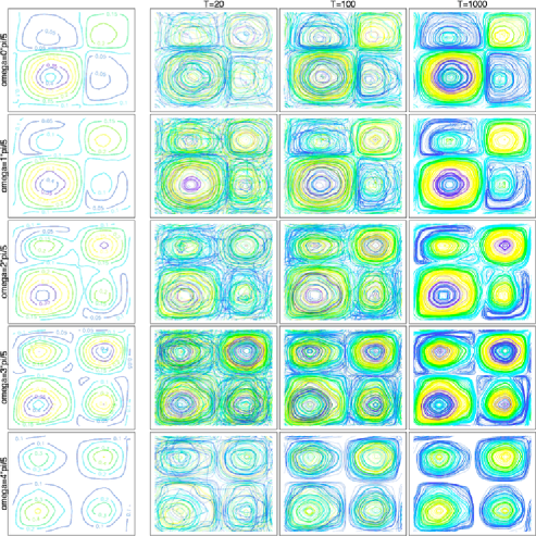
Figure 2: Contour plots for the amplitude of the true and estimated spectral density kernel when the innovation process consists of Wiener processes. Each row corresponds to a different frequency ($\omega=k\pi/5$, $k=0,1,\ldots,4$, going from top to bottom). The first column contains the contour plots of the true amplitudes of the kernel at each corresponding frequency. The rest of the columns correspond to the estimated contours for different sample sizes ($T=20,100,1000$ from left to right). Twenty estimates, corresponding to twenty replications of the process, have been superposed in order to provide a visual illustration of the variability. The contours plotted always correspond to the same level curves and use the same colour-coding in each row.

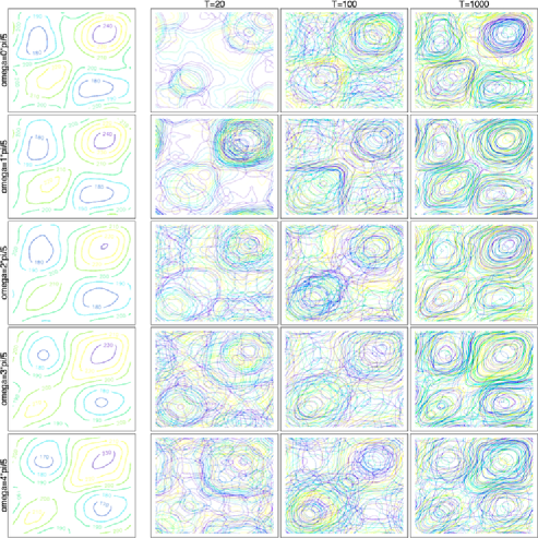
Figure 3: Contour plots for the amplitude of the true and estimated spectral density kernel when the innovation process consists of white noise processes. Each row corresponds to a different frequency ($\omega=k\pi/5$, $k=0,1,\ldots,4$, going from top to bottom). The first column contains the contour plots of the true amplitudes of the kernel at each corresponding frequency. The rest of the columns correspond to the estimated contours for different sample sizes ($T=20,100,1000$ from left to right). Twenty estimates, corresponding to twenty replications of the process, have been superposed in order to provide a visual illustration of the variability. The contours plotted always correspond to the same level curves and use the same colour-coding in each row.

In order to gain a visual appreciation of the accuracy of the estimators, we construct plots to compare the true and estimated spectral density kernels in Figures 2 and 3, for the Wiener and white noise cases, respectively. For practical purposes, we set $\alpha=2$, as for the simulation of the IMSEs. We simulated $X_{t}=A_{0}\varepsilon_{t}+A_{1}\varepsilon_{t-1}$, where $\varepsilon_{t}(\tau)$ lies on the subspace of $L^{2}([0,1],\mathbb{R})$ spanned by the basis $e_{1},\ldots,e_{100}$, and the operators $A_{0},A_{1}$ lie in the subspace spanned by $(\psi_{m}\otimes e_{k})_{m=1,\ldots,51;k=1,\ldots,100}$. Since the target parameter is a complex-valued function defined over a two-dimensional rectangle, some information loss must be incurred when representing it graphically. We chose to suppress the phase component of the spectral density kernel, plotting only its amplitude, $|\mathpzc{f}_{\omega}(\tau,\sigma)|$, for all $(\tau,\sigma)\in[0,1]^{2}$ and for selected frequencies $\omega$ (the spectral density kernel is seen to be smooth in $\omega$, so this does not entail a significant loss of information). For various choices of sample size $T$, we have replicated the realisation of the process, and the corresponding kernel density estimator for the particular frequency. Each time, we plotted the contours in superposition, in order to be able to visually appreciate the variability in the estimators: tangled contour lines where no clear systematic pattern emerges signify a region of high variability, whereas aligned contour lines that adhere to a recognisable shape represent regions of low variability. As is expected, the “smoother” the innovation process, the less variable the results appear to be, and the variability decreases for larger values of $T$.

7 Background results and technical statements

Statements and proofs of intermediate results in functional analysis and probability in function space that are required in our earlier formal derivations, can be found in the supplementary material [Panaretos and Tavakoli (2013)]. This supplement also collects some known results and facts for the reader’s ease. We include here a useful lemma that provides an easily verifiable $L^{2}$ moment condition that is sufficient for tightness to hold true. It collects arguments appearing in the proof of Bosq (2000), Theorem 2.7, and its proof can also be found in the supplementary material [Panaretos and Tavakoli (2013)].

Lemma 7.1 ((Criterion for tightness in Hilbert space)).

Let $H$ be a (real or complex) separable Hilbert space, and $X_{T}\dvtx\Omega\rightarrow H,T=1,2,\ldots,$ be a sequence of random variables. If for some complete orthonormal basis $\{e_{n}\}_{n\geq 1}$ of $H$, we have $\mathbb{E}|{\langle X_{T},e_{n}\rangle}|^{2}\leq a_{n},n=1,2,\ldots,$ for all large $T$, and $\sum_{n\geq 1}a_{n}<\infty,$ then $\{X_{T}\}_{T\geq 1}$ is tight.

References

- Adler (1990) {bbook}[mr] \bauthor\bsnmAdler, \bfnmRobert J.\binitsR. J. (\byear1990). \btitleAn Introduction to Continuity, Extrema, and Related Topics for General Gaussian Processes. \bseriesInstitute of Mathematical Statistics Lecture Notes—Monograph Series \bvolume12. \bpublisherIMS, \blocationHayward, CA. \bidmr=1088478 \bptokimsref \endbibitem
- Anderson (1994) {bbook}[mr] \bauthor\bsnmAnderson, \bfnmT. W.\binitsT. W. (\byear1994). \btitleThe Statistical Analysis of Time Series. \bpublisherWiley, \blocationNew York. \bptnotecheck year\bptokimsref \endbibitem
- Antoniadis, Paparoditis and Sapatinas (2006) {barticle}[mr] \bauthor\bsnmAntoniadis, \bfnmAnestis\binitsA., \bauthor\bsnmPaparoditis, \bfnmEfstathios\binitsE. and \bauthor\bsnmSapatinas, \bfnmTheofanis\binitsT. (\byear2006). \btitleA functional wavelet-kernel approach for time series prediction. \bjournalJ. R. Stat. Soc. Ser. B Stat. Methodol. \bvolume68 \bpages837–857. \biddoi=10.1111/j.1467-9868.2006.00569.x, issn=1369-7412, mr=2301297 \bptokimsref \endbibitem
- Antoniadis and Sapatinas (2003) {barticle}[mr] \bauthor\bsnmAntoniadis, \bfnmAnestis\binitsA. and \bauthor\bsnmSapatinas, \bfnmTheofanis\binitsT. (\byear2003). \btitleWavelet methods for continuous-time prediction using Hilbert-valued autoregressive processes. \bjournalJ. Multivariate Anal. \bvolume87 \bpages133–158. \biddoi=10.1016/S0047-259X(03)00028-9, issn=0047-259X, mr=2007265 \bptokimsref \endbibitem
- Benko, Härdle and Kneip (2009) {barticle}[mr] \bauthor\bsnmBenko, \bfnmMichal\binitsM., \bauthor\bsnmHärdle, \bfnmWolfgang\binitsW. and \bauthor\bsnmKneip, \bfnmAlois\binitsA. (\byear2009). \btitleCommon functional principal components. \bjournalAnn. Statist. \bvolume37 \bpages1–34. \biddoi=10.1214/07-AOS516, issn=0090-5364, mr=2488343 \bptokimsref \endbibitem
- Bloomfield (2000) {bbook}[mr] \bauthor\bsnmBloomfield, \bfnmPeter\binitsP. (\byear2000). \btitleFourier Analysis of Time Series: An Introduction, \bedition2nd ed. \bpublisherWiley, \blocationNew York. \biddoi=10.1002/0471722235, mr=1884963 \bptokimsref \endbibitem
- Boente, Rodriguez and Sued (2011) {bincollection}[mr] \bauthor\bsnmBoente, \bfnmGraciela\binitsG., \bauthor\bsnmRodriguez, \bfnmDaniela\binitsD. and \bauthor\bsnmSued, \bfnmMariela\binitsM. (\byear2011). \btitleTesting the equality of covariance operators. In \bbooktitleRecent Advances in Functional Data Analysis and Related Topics \bpages49–53. \bpublisherPhysica-Verlag/Springer, \baddressHeidelberg. \biddoi=10.1007/978-3-7908-2736-1_8, mr=2815560 \bptokimsref \endbibitem
- Bosq (2000) {bbook}[mr] \bauthor\bsnmBosq, \bfnmD.\binitsD. (\byear2000). \btitleLinear Processes in Function Spaces: Theory and Applications. \bseriesLecture Notes in Statistics \bvolume149. \bpublisherSpringer, \blocationNew York. \biddoi=10.1007/978-1-4612-1154-9, mr=1783138 \bptokimsref \endbibitem
- Bosq (2002) {barticle}[mr] \bauthor\bsnmBosq, \bfnmDenis\binitsD. (\byear2002). \btitleEstimation of mean and covariance operator of autoregressive processes in Banach spaces. \bjournalStat. Inference Stoch. Process. \bvolume5 \bpages287–306. \biddoi=10.1023/A:1021279131053, issn=1387-0874, mr=1943835 \bptokimsref \endbibitem
- Bosq and Blanke (2007) {bbook}[mr] \bauthor\bsnmBosq, \bfnmDenis\binitsD. and \bauthor\bsnmBlanke, \bfnmDelphine\binitsD. (\byear2007). \btitleInference and Prediction in Large Dimensions. \bpublisherWiley, \blocationChichester. \biddoi=10.1002/9780470724033, mr=2364006 \bptnotecheck year\bptokimsref \endbibitem
- Brillinger (2001) {bbook}[mr] \bauthor\bsnmBrillinger, \bfnmDavid R.\binitsD. R. (\byear2001). \btitleTime Series: Data Analysis and Theory. \bseriesClassics in Applied Mathematics \bvolume36. \bpublisherSIAM, \blocationPhiladelphia, PA. \biddoi=10.1137/1.9780898719246, mr=1853554 \bptokimsref \endbibitem
- Cardot and Sarda (2006) {bincollection}[mr] \bauthor\bsnmCardot, \bfnmHervé\binitsH. and \bauthor\bsnmSarda, \bfnmPascal\binitsP. (\byear2006). \btitleLinear regression models for functional data. In \bbooktitleThe Art of Semiparametrics \bpages49–66. \bpublisherPhysica-Verlag/Springer, \baddressHeidelberg. \biddoi=10.1007/3-7908-1701-5_4, mr=2234875 \bptokimsref \endbibitem
- Cuevas, Febrero and Fraiman (2002) {barticle}[mr] \bauthor\bsnmCuevas, \bfnmAntonio\binitsA., \bauthor\bsnmFebrero, \bfnmManuel\binitsM. and \bauthor\bsnmFraiman, \bfnmRicardo\binitsR. (\byear2002). \btitleLinear functional regression: The case of fixed design and functional response. \bjournalCanad. J. Statist. \bvolume30 \bpages285–300. \biddoi=10.2307/3315952, issn=0319-5724, mr=1926066 \bptokimsref \endbibitem
- Dauxois, Pousse and Romain (1982) {barticle}[mr] \bauthor\bsnmDauxois, \bfnmJ.\binitsJ., \bauthor\bsnmPousse, \bfnmA.\binitsA. and \bauthor\bsnmRomain, \bfnmY.\binitsY. (\byear1982). \btitleAsymptotic theory for the principal component analysis of a vector random function: Some applications to statistical inference. \bjournalJ. Multivariate Anal. \bvolume12 \bpages136–154. \biddoi=10.1016/0047-259X(82)90088-4, issn=0047-259X, mr=0650934 \bptokimsref \endbibitem
- Dehling and Sharipov (2005) {barticle}[mr] \bauthor\bsnmDehling, \bfnmHerold\binitsH. and \bauthor\bsnmSharipov, \bfnmOlimjon Sh.\binitsO. S. (\byear2005). \btitleEstimation of mean and covariance operator for Banach space valued autoregressive processes with dependent innovations. \bjournalStat. Inference Stoch. Process. \bvolume8 \bpages137–149. \biddoi=10.1007/s11203-003-0382-8, issn=1387-0874, mr=2121674 \bptokimsref \endbibitem
- Edwards (1967) {bbook}[auto:STB—2013/03/04—13:35:07] \bauthor\bsnmEdwards, \bfnmR.\binitsR. (\byear1967). \btitleFourier Series: A Modern Introduction. \bpublisherHolt, Rinehart & Winston, \blocationNew York. \bptokimsref \endbibitem
- Ferraty and Vieu (2004) {barticle}[mr] \bauthor\bsnmFerraty, \bfnmF.\binitsF. and \bauthor\bsnmVieu, \bfnmP.\binitsP. (\byear2004). \btitleNonparametric models for functional data, with application in regression, time-series prediction and curve discrimination. \bjournalJ. Nonparametr. Stat. \bvolume16 \bpages111–125. \biddoi=10.1080/10485250310001622686, issn=1048-5252, mr=2053065 \bptokimsref \endbibitem
- Ferraty and Vieu (2006) {bbook}[mr] \bauthor\bsnmFerraty, \bfnmFrédéric\binitsF. and \bauthor\bsnmVieu, \bfnmPhilippe\binitsP. (\byear2006). \btitleNonparametric Functional Data Analysis: Theory and Practice. \bpublisherSpringer, \blocationNew York. \bidmr=2229687 \bptokimsref \endbibitem
- Ferraty et al. (2011a) {bincollection}[mr] \bauthor\bsnmFerraty, \bfnmFrédéric\binitsF., \bauthor\bsnmGoia, \bfnmAldo\binitsA., \bauthor\bsnmSalinelli, \bfnmEnersto\binitsE. and \bauthor\bsnmVieu, \bfnmPhilippe\binitsP. (\byear2011a). \btitleRecent advances on functional additive regression. In \bbooktitleRecent Advances in Functional Data Analysis and Related Topics \bpages97–102. \bpublisherPhysica-Verlag/Springer, \baddressHeidelberg. \biddoi=10.1007/978-3-7908-2736-1_15, mr=2815567 \bptokimsref \endbibitem
- Ferraty et al. (2011b) {barticle}[mr] \bauthor\bsnmFerraty, \bfnmFrédéric\binitsF., \bauthor\bsnmLaksaci, \bfnmAli\binitsA., \bauthor\bsnmTadj, \bfnmAmel\binitsA. and \bauthor\bsnmVieu, \bfnmPhilippe\binitsP. (\byear2011b). \btitleKernel regression with functional response. \bjournalElectron. J. Stat. \bvolume5 \bpages159–171. \biddoi=10.1214/11-EJS600, issn=1935-7524, mr=2786486 \bptokimsref \endbibitem
- Fremdt et al. (2013) {barticle}[auto:STB—2013/03/04—13:35:07] \bauthor\bsnmFremdt, \bfnmS.\binitsS., \bauthor\bsnmSteinebach, \bfnmJ.\binitsJ., \bauthor\bsnmHorváth, \bfnmL.\binitsL. and \bauthor\bsnmKokoszka, \bfnmP.\binitsP. (\byear2013). \btitleTesting the equality of covariance operators in functional samples. \bjournalScand. J. Stat. \bvolume40 \bpages138–152. \bptokimsref \endbibitem
- Gabrys, Horváth and Kokoszka (2010) {barticle}[mr] \bauthor\bsnmGabrys, \bfnmRobertas\binitsR., \bauthor\bsnmHorváth, \bfnmLajos\binitsL. and \bauthor\bsnmKokoszka, \bfnmPiotr\binitsP. (\byear2010). \btitleTests for error correlation in the functional linear model. \bjournalJ. Amer. Statist. Assoc. \bvolume105 \bpages1113–1125. \biddoi=10.1198/jasa.2010.tm09794, issn=0162-1459, mr=2752607 \bptokimsref \endbibitem
- Gabrys and Kokoszka (2007) {barticle}[mr] \bauthor\bsnmGabrys, \bfnmRobertas\binitsR. and \bauthor\bsnmKokoszka, \bfnmPiotr\binitsP. (\byear2007). \btitlePortmanteau test of independence for functional observations. \bjournalJ. Amer. Statist. Assoc. \bvolume102 \bpages1338–1348. \biddoi=10.1198/016214507000001111, issn=0162-1459, mr=2412554 \bptokimsref \endbibitem
- Grenander (1981) {bbook}[mr] \bauthor\bsnmGrenander, \bfnmUlf\binitsU. (\byear1981). \btitleAbstract Inference. \bpublisherWiley, \blocationNew York. \bidmr=0599175 \bptokimsref \endbibitem
- Grenander and Rosenblatt (1957) {bbook}[mr] \bauthor\bsnmGrenander, \bfnmUlf\binitsU. and \bauthor\bsnmRosenblatt, \bfnmMurray\binitsM. (\byear1957). \btitleStatistical Analysis of Stationary Time Series. \bpublisherWiley, \blocationNew York. \bidmr=0084975 \bptnotecheck year\bptokimsref \endbibitem
- Hall and Hosseini-Nasab (2006) {barticle}[mr] \bauthor\bsnmHall, \bfnmPeter\binitsP. and \bauthor\bsnmHosseini-Nasab, \bfnmMohammad\binitsM. (\byear2006). \btitleOn properties of functional principal components analysis. \bjournalJ. R. Stat. Soc. Ser. B Stat. Methodol. \bvolume68 \bpages109–126. \biddoi=10.1111/j.1467-9868.2005.00535.x, issn=1369-7412, mr=2212577 \bptokimsref \endbibitem
- Hall and Vial (2006) {barticle}[mr] \bauthor\bsnmHall, \bfnmPeter\binitsP. and \bauthor\bsnmVial, \bfnmCéline\binitsC. (\byear2006). \btitleAssessing the finite dimensionality of functional data. \bjournalJ. R. Stat. Soc. Ser. B Stat. Methodol. \bvolume68 \bpages689–705. \biddoi=10.1111/j.1467-9868.2006.00562.x, issn=1369-7412, mr=2301015 \bptokimsref \endbibitem
- Hannan (1970) {bbook}[mr] \bauthor\bsnmHannan, \bfnmE. J.\binitsE. J. (\byear1970). \btitleMultiple Time Series. \bpublisherWiley, \blocationNew York. \bidmr=0279952 \bptokimsref \endbibitem
- Hörmann and Kokoszka (2010) {barticle}[mr] \bauthor\bsnmHörmann, \bfnmSiegfried\binitsS. and \bauthor\bsnmKokoszka, \bfnmPiotr\binitsP. (\byear2010). \btitleWeakly dependent functional data. \bjournalAnn. Statist. \bvolume38 \bpages1845–1884. \biddoi=10.1214/09-AOS768, issn=0090-5364, mr=2662361 \bptokimsref \endbibitem
- Horváth, Hušková and Kokoszka (2010) {barticle}[mr] \bauthor\bsnmHorváth, \bfnmLajos\binitsL., \bauthor\bsnmHušková, \bfnmMarie\binitsM. and \bauthor\bsnmKokoszka, \bfnmPiotr\binitsP. (\byear2010). \btitleTesting the stability of the functional autoregressive process. \bjournalJ. Multivariate Anal. \bvolume101 \bpages352–367. \biddoi=10.1016/j.jmva.2008.12.008, issn=0047-259X, mr=2564345 \bptokimsref \endbibitem
- Horváth and Kokoszka (2012) {bbook}[mr] \bauthor\bsnmHorváth, \bfnmLajos\binitsL. and \bauthor\bsnmKokoszka, \bfnmPiotr\binitsP. (\byear2012). \btitleInference for Functional Data with Applications. \bpublisherSpringer, \blocationNew York. \biddoi=10.1007/978-1-4614-3655-3, mr=2920735 \bptokimsref \endbibitem
- Horváth, Kokoszka and Reeder (2013) {barticle}[auto:STB—2013/03/04—13:35:07] \bauthor\bsnmHorváth, \bfnmL.\binitsL., \bauthor\bsnmKokoszka, \bfnmP.\binitsP. and \bauthor\bsnmReeder, \bfnmR.\binitsR. (\byear2013). \btitleEstimation of the mean of functional time series and a two-sample problem. \bjournalJ. R. Stat. Soc. Ser. B Stat. Methodol. \bvolume75 \bpages103–122. \bptokimsref \endbibitem
- Hunter and Nachtergaele (2001) {bbook}[mr] \bauthor\bsnmHunter, \bfnmJohn K.\binitsJ. K. and \bauthor\bsnmNachtergaele, \bfnmBruno\binitsB. (\byear2001). \btitleApplied Analysis. \bpublisherWorld Scientific, \blocationRiver Edge, NJ. \bidmr=1829589 \bptnotecheck year\bptokimsref \endbibitem
- Kadison and Ringrose (1997) {bbook}[auto:STB—2013/03/04—13:35:07] \bauthor\bsnmKadison, \bfnmR. V.\binitsR. V. and \bauthor\bsnmRingrose, \bfnmJ. R.\binitsJ. R. (\byear1997). \btitleFundamentals of the Theory of Operator Algebras. \bseriesGraduate Studies in Mathematics \bvolume15. \bpublisherAmer. Math. Soc., \blocationProvidence, RI. \bptokimsref \endbibitem
- Karhunen (1947) {barticle}[mr] \bauthor\bsnmKarhunen, \bfnmKari\binitsK. (\byear1947). \btitleÜber lineare Methoden in der Wahrscheinlichkeitsrechnung. \bjournalAnn. Acad. Sci. Fennicae. Ser. A I Math.-Phys. \bvolume1947 \bpages79. \bidmr=0023013 \bptokimsref \endbibitem
- Kolmogorov (1978) {bbook}[auto:STB—2013/03/04—13:35:07] \bauthor\bsnmKolmogorov, \bfnmA.\binitsA. (\byear1978). \btitleStationary Sequences in Hilbert Space. \bpublisherNational Translations Center [John Crerar Library], \blocationChicago. \bptokimsref \endbibitem
- Kraus and Panaretos (2012) {barticle}[auto:STB—2013/03/04—13:35:07] \bauthor\bsnmKraus, \bfnmD.\binitsD. and \bauthor\bsnmPanaretos, \bfnmV. M.\binitsV. M. (\byear2012). \btitleDisperson operators and resistant second-order functional data analysis. \bjournalBiometrika \bvolume99 \bpages813–832. \bptokimsref \endbibitem
- Laib and Louani (2010) {barticle}[mr] \bauthor\bsnmLaib, \bfnmNaâmane\binitsN. and \bauthor\bsnmLouani, \bfnmDjamal\binitsD. (\byear2010). \btitleNonparametric kernel regression estimation for functional stationary ergodic data: Asymptotic properties. \bjournalJ. Multivariate Anal. \bvolume101 \bpages2266–2281. \biddoi=10.1016/j.jmva.2010.05.010, issn=0047-259X, mr=2719861 \bptokimsref \endbibitem
- Ledoux and Talagrand (1991) {bbook}[mr] \bauthor\bsnmLedoux, \bfnmMichel\binitsM. and \bauthor\bsnmTalagrand, \bfnmMichel\binitsM. (\byear1991). \btitleProbability in Banach Spaces: Isoperimetry and Processes. \bseriesErgebnisse der Mathematik und Ihrer Grenzgebiete (3) [Results in Mathematics and Related Areas (3)] \bvolume23. \bpublisherSpringer, \blocationBerlin. \bidmr=1102015 \bptokimsref \endbibitem
- Lévy (1948) {bbook}[mr] \bauthor\bsnmLévy, \bfnmPaul\binitsP. (\byear1948). \btitleProcessus stochastiques et mouvement Brownien. Suivi d’une note de M. Loève. \bpublisherGauthier-Villars, \blocationParis. \bidmr=0029120 \bptokimsref \endbibitem
- Liu and Wu (2010) {barticle}[mr] \bauthor\bsnmLiu, \bfnmWeidong\binitsW. and \bauthor\bsnmWu, \bfnmWei Biao\binitsW. B. (\byear2010). \btitleAsymptotics of spectral density estimates. \bjournalEconometric Theory \bvolume26 \bpages1218–1245. \biddoi=10.1017/S026646660999051X, issn=0266-4666, mr=2660298 \bptokimsref \endbibitem
- Locantore et al. (1999) {barticle}[mr] \bauthor\bsnmLocantore, \bfnmN.\binitsN., \bauthor\bsnmMarron, \bfnmJ. S.\binitsJ. S., \bauthor\bsnmSimpson, \bfnmD. G.\binitsD. G., \bauthor\bsnmTripoli, \bfnmN.\binitsN., \bauthor\bsnmZhang, \bfnmJ. T.\binitsJ. T. and \bauthor\bsnmCohen, \bfnmK. L.\binitsK. L. (\byear1999). \btitleRobust principal component analysis for functional data. \bjournalTEST \bvolume8 \bpages1–73. \biddoi=10.1007/BF02595862, issn=1133-0686, mr=1707596 \bptnotecheck related\bptokimsref \endbibitem
- Mas (2000) {bmisc}[auto:STB—2013/03/04—13:35:07] \bauthor\bsnmMas, \bfnmA.\binitsA. (\byear2000). \bhowpublishedEstimation d’opérateurs de corrélation de processus linéaires fonctionnels: lois limites, déviations modérées. Ph.D. thesis, Université Paris VI. \bptokimsref \endbibitem
- Panaretos, Kraus and Maddocks (2010) {barticle}[mr] \bauthor\bsnmPanaretos, \bfnmVictor M.\binitsV. M., \bauthor\bsnmKraus, \bfnmDavid\binitsD. and \bauthor\bsnmMaddocks, \bfnmJohn H.\binitsJ. H. (\byear2010). \btitleSecond-order comparison of Gaussian random functions and the geometry of DNA minicircles. \bjournalJ. Amer. Statist. Assoc. \bvolume105 \bpages670–682. \biddoi=10.1198/jasa.2010.tm09239, issn=0162-1459, mr=2724851 \bptokimsref \endbibitem
- Panaretos and Tavakoli (2013) {bmisc}[auto:STB—2013/03/04—13:35:07] \bauthor\bsnmPanaretos, \bfnmV. M.\binitsV. M. and \bauthor\bsnmTavakoli, \bfnmS.\binitsS. (\byear2013). \bhowpublishedCramér–Karhunen–Loève representation and harmonic principal component analysis of functional time series. Stochastic Process. Appl. To appear. DOI:\doiurl10.1016/j.spa.2013.03.015, available at http://www.sciencedirect.com/science/article/pii/S0304414913000793. \bptokimsref \endbibitem
- Panaretos and Tavakoli (2013) {bmisc}[auto] \bauthor\bsnmPanaretos, \bfnmV. M.\binitsV. M. and \bauthor\bsnmTavakoli, \bfnmS.\binitsS. (\byear2013). \bhowpublishedSupplement to “Fourier analysis of stationary time series in function space.” DOI:\doiurl10.1214/13-AOS1086SUPP. \bptokimsref \endbibitem
- Peligrad and Wu (2010) {barticle}[mr] \bauthor\bsnmPeligrad, \bfnmMagda\binitsM. and \bauthor\bsnmWu, \bfnmWei Biao\binitsW. B. (\byear2010). \btitleCentral limit theorem for Fourier transforms of stationary processes. \bjournalAnn. Probab. \bvolume38 \bpages2009–2022. \biddoi=10.1214/10-AOP530, issn=0091-1798, mr=2722793 \bptokimsref \endbibitem
- Pollard (1984) {bbook}[mr] \bauthor\bsnmPollard, \bfnmDavid\binitsD. (\byear1984). \btitleConvergence of Stochastic Processes. \bpublisherSpringer, \blocationNew York. \biddoi=10.1007/978-1-4612-5254-2, mr=0762984 \bptokimsref \endbibitem
- Priestley (2001) {bbook}[auto:STB—2013/03/04—13:35:07] \bauthor\bsnmPriestley, \bfnmM. B.\binitsM. B. (\byear2001). \btitleSpectral Analysis and Time Series, Vol. I and II. \bpublisherAcademic Press, \blocationSan Diego. \bptokimsref \endbibitem
- Ramsay and Silverman (2005) {bbook}[mr] \bauthor\bsnmRamsay, \bfnmJ. O.\binitsJ. O. and \bauthor\bsnmSilverman, \bfnmB. W.\binitsB. W. (\byear2005). \btitleFunctional Data Analysis, \bedition2nd ed. \bpublisherSpringer, \blocationNew York. \bidmr=2168993 \bptokimsref \endbibitem
- Rice and Silverman (1991) {barticle}[mr] \bauthor\bsnmRice, \bfnmJohn A.\binitsJ. A. and \bauthor\bsnmSilverman, \bfnmB. W.\binitsB. W. (\byear1991). \btitleEstimating the mean and covariance structure nonparametrically when the data are curves. \bjournalJ. Roy. Statist. Soc. Ser. B \bvolume53 \bpages233–243. \bidissn=0035-9246, mr=1094283 \bptokimsref \endbibitem
- Rosenblatt (1984) {barticle}[mr] \bauthor\bsnmRosenblatt, \bfnmM.\binitsM. (\byear1984). \btitleAsymptotic normality, strong mixing and spectral density estimates. \bjournalAnn. Probab. \bvolume12 \bpages1167–1180. \bidissn=0091-1798, mr=0757774 \bptokimsref \endbibitem
- Rosenblatt (1985) {bbook}[mr] \bauthor\bsnmRosenblatt, \bfnmMurray\binitsM. (\byear1985). \btitleStationary Sequences and Random Fields. \bpublisherBirkhäuser, \blocationBoston, MA. \biddoi=10.1007/978-1-4612-5156-9, mr=0885090 \bptokimsref \endbibitem
- Sen and Klüppelberg (2010) {bmisc}[auto:STB—2013/03/04—13:35:07] \bauthor\bsnmSen, \bfnmR.\binitsR. and \bauthor\bsnmKlüppelberg, \bfnmC.\binitsC. (\byear2010). \bhowpublishedTime series of functional data. Unpublished manuscript. Available at http://citeseerx.ist.psu.edu/viewdoc/summary?doi= 10.1.1.185.2739. \bptokimsref \endbibitem
- Shao and Wu (2007) {barticle}[mr] \bauthor\bsnmShao, \bfnmXiaofeng\binitsX. and \bauthor\bsnmWu, \bfnmWei Biao\binitsW. B. (\byear2007). \btitleAsymptotic spectral theory for nonlinear time series. \bjournalAnn. Statist. \bvolume35 \bpages1773–1801. \biddoi=10.1214/009053606000001479, issn=0090-5364, mr=2351105 \bptokimsref \endbibitem
- Wand and Jones (1995) {bbook}[mr] \bauthor\bsnmWand, \bfnmM. P.\binitsM. P. and \bauthor\bsnmJones, \bfnmM. C.\binitsM. C. (\byear1995). \btitleKernel Smoothing. \bseriesMonographs on Statistics and Applied Probability \bvolume60. \bpublisherChapman & Hall, \blocationLondon. \bidmr=1319818 \bptokimsref \endbibitem
- Weidmann (1980) {bbook}[mr] \bauthor\bsnmWeidmann, \bfnmJoachim\binitsJ. (\byear1980). \btitleLinear Operators in Hilbert Spaces. \bseriesGraduate Texts in Mathematics \bvolume68. \bpublisherSpringer, \blocationNew York. \bidmr=0566954 \bptokimsref \endbibitem
- Wheeden and Zygmund (1977) {bbook}[mr] \bauthor\bsnmWheeden, \bfnmRichard L.\binitsR. L. and \bauthor\bsnmZygmund, \bfnmAntoni\binitsA. (\byear1977). \btitleMeasure and Integral: An Introduction to Real Analysis. \bseriesPure and Applied Mathematics \bvolume43. \bpublisherDekker, \blocationNew York. \bidmr=0492146 \bptokimsref \endbibitem
- Yao, Müller and Wang (2005) {barticle}[mr] \bauthor\bsnmYao, \bfnmFang\binitsF., \bauthor\bsnmMüller, \bfnmHans-Georg\binitsH.-G. and \bauthor\bsnmWang, \bfnmJane-Ling\binitsJ.-L. (\byear2005). \btitleFunctional linear regression analysis for longitudinal data. \bjournalAnn. Statist. \bvolume33 \bpages2873–2903. \biddoi=10.1214/009053605000000660, issn=0090-5364, mr=2253106 \bptokimsref \endbibitem