Planar massless fermions in Coulomb and Aharonov-Bohm potentials

Abstract

Solutions to the Dirac equation are constructed for a massless charged fermion in Coulomb and Aharonov–Bohm potentials in 2+1 dimensions. The Dirac Hamiltonian on this background is singular and needs a one-parameter self-adjoint extension, which can be given in terms of self-adjoint boundary conditions. We show that the virtual (quasistationary) bound states emerge in the presence of an attractive Coulomb potential when the so-called effective charges become overcritical and discuss a restructuring of the vacuum of the quantum electrodynamics when the virtual bound states emerge. We derive equations, which determine the energies and lifetimes of virtual bound states, find solutions of obtained equations for some values of parameters as well as analyze the local density of states as a function of energy in the presence of Coulomb and Aharonov–Bohm potentials.

.

I Introduction

Huge interest to different effects in the two-dimensional (2D) systems has appeared recently after successful fabrication of a monolayer graphite (graphene)(see netall and fine Reviews ngpng ; kupgc ). The single electron dynamics in graphene is described by a massless two-component Dirac equation ngpng ; ksn ; zji ; vpnn ; ashkl ; ifh and so massless Dirac excitations in graphene gnn can provide an interesting realization of quantum electrodynamics in 2+1 dimensions ggvo ; ggvo1 . Since, the “effective fine structure constant” in graphene is large, there appears a new possibility to study a strong-coupling version of the quantum electrodynamics (QED). The induced current in the graphene in the field of solenoid perpendicular to the plane of a sample was found to be a finite periodical function of the magnetic flux of solenoid jmpt . Coulomb impurity problems, such as the vacuum polarization and screening, in graphene were studied in vpnn ; ashkl ; tmksh . Solutions to the Dirac equation with an Aharonov–Bohm potential in 2+1 dimensions were also applied in a study of the interaction of cosmic strings with matter aw . The Dirac Hamiltonians for the above problems are essentially singular and so the supplementary definition is required in order for they to be treated as self-adjoint quantum-mechanical operators; it is necessary to indicate the Hamiltonian domain in the Hilbert space of square-integrable functions.

An important example of a singular Dirac Hamiltonian is the one in a strong Coulomb field of a point-like charge described by $4$ - potential: $A^{0}(r)=a/e_{0}r,{\bf A}=0,a>0,e_{0}>0$ (where $-e_{0}$ is the electron charge). We remind that the lowest bound state energy $E=m\sqrt{1-a^{2}}$ ($m$ is the electron mass) becomes purely imaginary for $a>1$, which implies that its interpretation as electron energy becomes meaningless, indicates that the Hamiltonian of the system is not a self-adjoint operator for $a>1$ and should be extended to become a self-adjoint operator. The latter problem are usually solving (see, fine monograph grrein ) by replacing the singular $a/e_{0}r$ potential by a Coulomb potential cut off at small distances $R$. In such a field, when $a$ increases, the energies of discrete states approach the boundary of lower energy continuum, $E=-m$, and dive into the lower continuum. Then, discrete states turn into resonances with finite lifetimes, which can be described as quasistationary states with “complex energies”. Therefore, an electron-positron pair is created from the vacuum: the positron goes to infinity and the electron is coupled to the Coulomb center. The so-called critical charge $a_{cr}$ is determined by the condition of appearance of nonzero imaginary part of the energy. For massless charged fermions in the regularized Coulomb potential, there are no discrete levels for $a<1$ due to scale invariance of the massless Dirac equation, nevertheless for $a>1$ quasistationary states emerge kupgc ; ashkl ; fgms ; skl2 ; ggg ; gs .

Here we present a physically rigorous quantum-mechanical treatment of a motion of a massless charged fermion in Coulomb and Aharonov–Bohm potentials in 2+1 dimensions. We stress that the presence of the AB potential allows us to study the influence of the particle spin on the fermion states, which is due to the interaction between the electron spin magnetic moment and the AB magnetic field. This Dirac Hamiltonian is symmetric operator so the problem arises to construct all the self-adjoint extensions of a given symmetric operator and then to choose correct self-adjoint extensions by means of physical conditions. We construct the self-adjoint radial Dirac Hamiltonians on the above background by the asymmetry form method vgt originated from von Neumann theory of self-adjoint extensions.

II Solutions of the radial Dirac Hamiltonian

The space of particle quantum states in two spatial dimensions is the Hilbert space $\mathfrak{H}=L^{2}(\mathbb{R}^{2})$ of square-integrable functions $\Psi({\bf r}),{\bf r}=(x,y)$ with the scalar product

$$(\Psi_{1},\Psi_{2})=\int\Psi_{1}^{\dagger}({\bf r})\Psi_{2}({\bf r})d{\bf r},\quad d{\bf r}=dxdy.$$ (1)

The Dirac Hamiltonian for a massless fermion of charge $e=-e_{0}<0$ in an ($A_{\mu}$) Aharonov–Bohm $A_{0}=0$, $A_{r}=0$, $A_{\varphi}=B/r$, $r=\sqrt{x^{2}+y^{2}}$, $\varphi=\arctan(y/x)$ and Coulomb $A_{0}(r)=a/e_{0}r$, $A_{r}=0$, $A_{\varphi}=0$, $a>0$ potentials, is

$$H_{D}=\sigma_{1}P_{2}-s\sigma_{2}P_{1}+\sigma_{3}U(r)-e_{0}A_{0}(r),$$ (2)

where $P_{\mu}=-i\partial_{\mu}-eA_{\mu}$ is the generalized fermion momentum operator. The Dirac $\gamma^{\mu}$-matrix algebra is known to be represented in terms of the two-dimensional Pauli matrices $\sigma_{j}$ and the parameter $s=\pm 1$ can be introduced to label two types of fermions in accordance with the signature of the two-dimensional Dirac matrices hoso and is applied to characterize two states of the fermion spin (spin “up” and “down”) crh ; khlee .

The Hamiltonian (2) should be defined as a self-adjoint operator in the Hilbert space of square-integrable two-spinors $\Psi({\bf r}),{\bf r}=(x,y)$ with the scalar product (1). The total angular momentum $J\equiv L_{z}+s\sigma_{3}/2$, where $L_{z}\equiv-i\partial/\partial\varphi$, commutes with $H_{D}$, therefore, we can consider (2) separately in each eigenspace of the operator $J$ and the total Hilbert space is a direct orthogonal sum of subspaces of $J$.

Eigenfunctions of the Hamiltonian (2) are (see, hkh ; khlee1 )

$$\Psi(t,{\bf r})=\frac{1}{\sqrt{2\pi r}}\left(\begin{array}[]{c}f_{1}(r)\\ f_{2}(r)e^{is\varphi}\end{array}\right)\exp(-iEt+il\varphi)~{},$$ (5)

where $E$ is the fermion energy, $l$ is an integer. The wave function $\Psi$ is an eigenfunction of the operator $J$ with eigenvalue $j=l+s/2$ and the doublet

$$F=\left(\begin{array}[]{c}f_{1}(r)\\ f_{2}(r)\end{array}\right)$$ (8)

satisfies the equation

$$\check{h}F=EF$$ (9)

with

$$\check{h}=is\sigma_{2}\frac{d}{dr}+\sigma_{1}\frac{l+\mu+s/2}{r}-\frac{a}{r},\quad\mu\equiv e_{0}B$$ (10)

Thus, the problem is reduced to that for the radial Hamiltonian $\check{h}$ in the Hilbert space of doublets $F(r)$ square-integrable on the half-line.

In the real physical space because of the existence of the AB magnetic field ${\bf H}=(0,\,0,\,H)=\nabla\times{\bf A}=\pi B\delta({\bf r})$ there emerges the interaction of the fermion spin magnetic moment with the AB magnetic field in the form $-seB\delta(r)/r$. The additional (spin) singular potential will reveal itself only in the Dirac equation squared. The “spin” potential is invariant under the changes $e\to-e,s\to-s$, and it hence suffices to consider only the case $e=-e_{0}<0$ and $eB\equiv-\mu<0$. Then, the potential is attractive for $s=-1$ and repulsive for $s=1$. The influence of this singular potential on the behavior of solutions at the origin, in fact, is taken into account by means of boundary conditions.

An operator, associated with the so-called differential expression $\check{h}$, we shall denote by $h$. Let $\mathfrak{H}=\mathfrak{L}^{2}(0,\infty)$ be the Hilbert space of doublets $F(r)$, $G(r)$ with the scalar product

$$(F,G)=\int\limits_{0}^{\infty}F^{\dagger}(r)G(r)dr=\int\limits_{0}^{\infty}[\bar{f}_{1}(r)g_{1}(r)+\bar{f}_{2}(r)g_{2}(r)]dr,$$

so that $\mathfrak{L}^{2}(0,\infty)=L^{2}(0,\infty)\oplus L^{2}(0,\infty)$. Here the symbol $\oplus$ denotes the direct sum. Let us just define the operator $h^{0}$ in the Hilbert space $\mathfrak{L}^{2}(0,\infty)$

$$h^{0}{:}\left\{\begin{array}[]{l}D(h^{0})={\mathfrak{D}}(0,\infty),\\ h^{0}F(r)=\check{h}F(r),\end{array}\right.$$

where ${\mathfrak{D}}(0,\infty)=D(0,\infty)\oplus D(0,\infty)$, $D(0,\infty)$ is the standard space of smooth functions on $(0,\infty)$ with the compact support

$$D(0,\infty)={f(r):f(r)\in C^{\infty},\;{\rm supp}f\subset[c,d],\;0<c<d<\infty}.$$

This allows us to avoid the problems related to $r\to\infty$.

The operator $h$ is symmetric if for any $F(r)$ and $G(r)$

$$\int\limits_{0}^{\infty}G^{\dagger}(r)hF(r)rdr=\int\limits_{0}^{\infty}[hG(r)]^{\dagger}F(r)rdr.$$ (11)

We see that $h^{0}$ is the symmetric operator. Let $h$ be the self-adjoint extension $h^{0}$ in $\mathfrak{L}^{2}(0,\infty)$ and consider the adjoint operator $h^{*}$ (10) defined by

$$h^{*}{:}\left\{\begin{array}[]{l}D(h^{*})=\left\{\begin{array}[]{l}F(r):F(r)\;\mbox{is absolutely continuous in}(0,\infty),\\ F,\;\check{h}F=G\in{\mathfrak{L}}^{2}(0,\infty),\end{array}\right.\\ h^{*}F(r)=\check{h}F(r),\end{array}\right.$$

i.e. $D(h^{0})\subset D(h^{*})$. Since the coefficient functions of (10) are real, the deficiency indices of the operator $h^{0}$ are equal so that the self-adjoint extensions of $h^{0}$ exist at any values of parameters $a,\mu$, and for each $l$. A symmetric operator $h$ is self-adjoint, if its domain $D(h)$ coincides with that of its adjoint operator $D(h^{*})$.

Integrating (11) by parts and taking into account that for any doublet $F(r)$ of $D(h^{*})$ $\lim\limits_{r\to\infty}F(r)=0$, Eq. (11) is reduced to

$$\lim_{r\to 0}G^{\dagger}(r)i\sigma_{2}F(r)=0.$$ (16)

If (16) is satisfied for any doublets from $D(h^{*})\equiv D^{*}$ then the operator $h^{*}$ is symmetric and, so, self-adjoint. This means that the operator $h^{0}$ is essentially self-adjoint, i.e., its unique self-adjoint extension is its closure $h=\bar{h}^{0}$, which coincides with the adjoint operator $h=h^{*}=h^{\dagger}$. If (16) is not satisfied then the self-adjoint operator $h=h^{\dagger}$ can be found as the narrowing of $h^{*}$ on the so-called maximum domain $D(h)\subset D(h^{*})$ vgt .

The needed solution of (9) is

$$F =e^{-x/2}r^{\gamma_{s}}A^{\prime}\left[v_{+}\Phi(a^{s},\;c_{s}\;;x)+v_{-}m_{s}\Phi(a^{s}+s,\;c_{s}\;;x)\right]$$

$$\equiv AY(r,\gamma_{s},E).$$ (17)

Here $A^{\prime}$, $A$ are constants, $x=-2i|E|r$, $a^{s}=\gamma_{s}+(1-s)/2-ie^{\prime}a$, $c_{s}=2\gamma_{s}+1$, $e^{\prime}=E/|E|$, $\gamma_{s}=\pm\sqrt{(l+\mu+s/2)^{2}-a^{2}}\equiv\gamma_{s}^{\pm}$, $m_{s}=(s\gamma-ie^{\prime}a)/\nu,\nu=l+\mu+s/2$,

$$v_{+}=\left(\begin{array}[]{c}1\\ -ie^{\prime}\end{array}\right),\quad v_{-}=\left(\begin{array}[]{c}1\\ ie^{\prime}\end{array}\right),$$ (22)

$\Phi(a,c;x)$ is the confluent hypergeometric function GR .

We denote $\gamma_{s}^{+}=\sqrt{\nu^{2}-a^{2}}\equiv\gamma$ for $a^{2}\leq\nu^{2}$ and $\gamma_{s}^{+}=i\sqrt{a^{2}-\nu^{2}}\equiv i\sigma$ for $a^{2}>\nu^{2}$. Then, for $\gamma\neq n/2$, $n=1,2,\ldots$, needed linear independent solutions are:

$$U_{1}(r;E) =Y(r,\gamma_{s},E)|_{\gamma_{s}=\gamma},$$

$$U_{2}(r;E) =Y(r,\gamma_{s},E)|_{\gamma_{s}=-\gamma}$$ (23)

with the asymptotic behavior at $r\to 0$

$$U_{1}(r;E) =r^{\gamma}u_{+}{+}O(r^{\gamma+1}),$$

$$U_{2}(r;E) =r^{-\gamma}u_{-}{+}O(r^{-\gamma+1})$$ (24)

as well as

$$V_{1}(r;E)=U_{1}(r;E)+\frac{a}{2s\gamma}\omega(E)U_{2}(r;E),$$ (25)

where $\omega(E)={\rm Wr}(U_{1},V_{1})$ is the Wronskian:

$$\omega(E)= \frac{\Gamma(2\gamma)\Gamma\left(-\gamma+(1-s)/2-ia\right)}{\Gamma(-2\gamma)\Gamma\left(\gamma+(1-s)/2-ia\right)}\times$$

$$\times(-2iE)^{-2\gamma}\frac{\nu+ia+s\gamma}{\nu+ia-s\gamma}\frac{2s\gamma}{a}.$$ (26)

The domain of the operator $h=h^{\dagger}$ is found as the narrowing of $h^{*}$ on the domain $D(h)\subset D^{*}$, so any doublet of $D(h)$ must satisfy the boundary condition (16)

$$(F^{\dagger}(r)i\sigma_{2}F(r))|_{r=0}=(\bar{f}_{1}f_{2}-\bar{f}_{2}f_{1})|_{r=0}=0.$$ (27)

Let us write $q=\sqrt{\nu^{2}-\gamma^{2}}$ and $q_{u}=\sqrt{\nu^{2}-1/4}\Leftrightarrow\gamma=1/2,\quad q_{c}=\nu\Leftrightarrow\gamma=0$. The quantity $q$ as a function of $l,a,\mu,s$ plays a role of the effective charge and $q_{c}$ is called the critical charge, which is affected by the magnetic flux and the particle spin.

III Subcritical range ($q<q_{c}$). Self-adjoint boundary conditions

By means of solutions $U_{1}(r)$ and $U_{2}(r)$ any doublet of $D^{*}$ can be represented in the form (see, vgt )

$$F(r)=c_{1}U_{1}(r)+c_{2}U_{2}(r)+I_{1}(r)+I_{2}(r),$$ (28)

where $c_{1}$ and $c_{2}$ - are some constants and $I_{1}(r)$, $I_{2}(r)$ are determined by integrals over $y$ of the tensor product $[U_{1}(r)\otimes{U}_{2}(y)]$. Asymptotic behavior of $F(r)$ at $r\to 0$ essentially depends on $\gamma$.

For $\gamma>0$ ($q<q_{u}$), $I_{1}(r)$ and $I_{2}(r)$ are khlee1

$$I_{1}(r)=O(r^{1/2}),\quad I_{2}(r)=O(r^{1/2}),\quad r\rightarrow{0}.$$ (29)

It follows that $F(r)\in{\mathfrak{L}}^{2}(0,\infty)$ implies $c_{2}=0$

$$F(r)=c_{1}U_{1}(r)+I_{1}(r)+I_{2}(r)=O(r^{1/2})\rightarrow{0},\;r\rightarrow{0}.$$ (30)

Then $F{\in}D^{*}$ and Eq. (27) is satisfied for $q\leq q_{u}$, $\gamma\geq 1/2$, which means that the initial symmetric operator $h$ is essentially self-adjoint and its unique self-adjoint extension is $h=h^{\dagger}$. Its domain $D(h)$ is the space of absolutely continuous doublets $F(r)$ regular at $r=0$ with $hF(r)$ belonging to $\mathfrak{L}^{2}(0,\infty)$.

For $0<\gamma<1/2$ ($q_{u}<q<q_{c}$) the left-hand side of (27) is $(\bar{f}_{1}f_{2}-\bar{f}_{2}f_{1})|_{r=0}=(2s\gamma/a)(\bar{c}_{1}c_{2}-\bar{c}_{2}c_{1})$, or, by means of the linear transformation $c_{1,2}\rightarrow{c_{\pm}}=c_{1}\pm{ic_{2}}$, is reduced to $(\bar{f}_{1}f_{2}-\bar{f}_{2}f_{1})|_{r=0}=-i(s\gamma/a)(|c_{+}|^{2}-|c_{-}|^{2})$. Hence, the operator $h^{*}$ is not symmetric and we need to construct the nontrivial self-adjoint extensions of $h^{0}$. Equation (27) will be satisfied for any $c_{-}$ related to $c_{+}$ by $c_{-}=e^{i\theta}c_{+}$ and $0\leq\theta\leq{2\pi}$, $0\thicksim{2\pi}$. The angle $\theta$ parameterizes the self-adjoint extensions $h_{\theta}$ of $h^{0}$. These extensions vary for different $\theta$ except for two equivalent cases $\theta=0$ and $\theta=2\pi$. We denote $\xi=\tan(\theta/2)$, then $c_{2}=-\xi{c_{1}}$, $-\infty\leq\xi\leq+\infty$, ${-\infty}\thicksim{+\infty}$.

Hence, in the range $0<\gamma<1/2$ there is one-parameter $U(1)$-family of the operators $h_{\theta}\equiv h_{\xi}$ with the domain $D_{\xi}$

$$h_{\xi}{:}\left\{\begin{array}[]{l}D_{\xi}=\left\{\begin{array}[]{l}F(r):F(r)\;\mbox{is absolutely continuous in}[0,\infty),\\ F,\check{h}F\in{\mathfrak{L}}^{2}(0,\infty),\\ F(r)=c[r^{\gamma}{u_{+}}-\xi r^{-\gamma}u_{-}]+O(r^{1/2}),\;|\xi|<\infty,\\ F(r)=cr^{-\gamma}u_{-}{+}O(r^{1/2}),\;r\rightarrow{0},\;\xi=\infty,\end{array}\right.\\ h_{\xi}F=\check{h}F,\end{array}\right.$$

where $c$ is arbitrary constant. The operator $h^{0}$ is not determined as an unique self-adjoint operator and so the additional specification of its domain, given with the real parameter $\xi$, is required in terms of the self-adjoint boundary conditions. Physically, the self-adjoint boundary conditions show that the probability current density is equal to zero at the origin.

The spectrum of the radial Hamiltonian is determined by the equation (see vgt ; khlee1 )

$$\frac{d\sigma(E)}{dE}=\frac{1}{\pi}\lim\limits_{\epsilon\rightarrow{0}}{\rm Im}\frac{1}{\omega_{\xi}(E+i\epsilon)},$$ (36)

where the generalized function $\omega_{\xi}(E+i\epsilon)$ is obtained by the analytic continuation of the corresponding Wronskian in the complex plane of $E$; on the real axis of $E$ it is just the function $\omega(E)$ determined by (26) for $\xi=0$. We note that Eq. (26) is obtained from the corresponding Wronskian for a fermion of mass $m>0$ in the limit $m\to 0$. Then, the Wronskians involve the variable $\lambda=\sqrt{m^{2}-E^{2}}$ and are characterized by two cuts $(-\infty,-m]$ and $[m,\infty)$ in the complex plane of $E$, which allows us to determine the first (physical) sheet (${\rm Re}\lambda>0$) and the second (unphysical) sheet (${\rm Re}\lambda<0$).

For $0<\gamma<1/2$ the doublet $U_{\xi}(r;E)$ should be chosen in the form

$$U_{\xi}(r;E)=U_{1}(r;E)-\xi U_{2}(r;E)$$ (37)

with asymptotic behavior at $r\to 0$ $U_{\xi}(r;E)=r^{\gamma}u_{+}-\xi r^{-\gamma}u_{-}+O(r^{-\gamma+1})$. Solution $V_{1}$ is now $V_{1}(r;E)\equiv V_{\xi}=U_{\xi}(r;E)+[a/2s\gamma]\omega_{\xi}(E)U_{2}(r;E)$ with $\omega_{\xi}(E)={\rm Wr}(U_{\xi},V_{\xi})=\omega(E)+2s\gamma\xi/a$ and $\omega(E)$ determined by (26). So $\omega_{\xi}(E)=\lim\limits_{\epsilon\rightarrow{0}}{\omega}_{\xi}(E+i\epsilon)$ and, thus, the spectral function is determined by the generalized function $F(E)=\lim\limits_{\epsilon\rightarrow{0}}{\omega}_{\xi}^{-1}(E+i\epsilon)$. At the points, at which the function ${\omega}_{\xi}(E)=\lim\limits_{\epsilon\rightarrow{0}}{\omega}_{\xi}(E+i\epsilon)$ is not equal zero $F(E)=1/\omega_{\xi}(E)$. It can be easily verified that the functions $\omega(E)$ and $\omega_{\xi}(E)$ are continuous, complex-valued and not equal to zero for real $E$; the spectral function $\sigma(E)$ exists and is absolutely continuous. Thus, the energy spectrum is continuous and the quantum system under discussion does not have bound states. Bound states would exist if $\omega_{\xi}(E)$ were real and the energy spectrum was determined by $\omega_{\xi}(E)=0$. One knows that real bound states (if they exist) are situated on the physical sheet of $\lambda$.

We shall suppose that the virtual bound (quasistationary) states “exist” on the unphysical sheet if their “energies” are determined by roots of equation $\omega_{\xi}(E)=0$. For $0<\gamma<1/2$, one can obtain for the real part of ${\rm Re}\omega_{\xi}(E)=0$

$$E=\frac{e^{\prime}}{2}\left[\frac{\Gamma(1+2\gamma)|\Gamma(-\gamma-ia)|}{|\xi|\Gamma(1-2\gamma)|\Gamma(\gamma-ia)|}\sqrt{\frac{\nu+s\gamma}{\nu-s\gamma}}\right]^{1/2\gamma}$$ (38)

and the following equation for ${\rm Im}\omega_{\xi}(E)=0$

$$\pi\left(e^{\prime}\gamma-\frac{1}{2}\right)-\frac{3+s}{4}\arctan\frac{4a\gamma}{4\gamma^{2}-(1+\nu^{2})(1-s)}+$$

$$+\sum\limits_{n=1}^{\infty}\arctan\frac{8a\gamma}{(2n+1-s)^{2}+4(a^{2}-\gamma^{2})}=(p-1)\frac{\pi}{2}.$$ (39)

Here $p=\xi/|\xi|=\pm 1$, $p=1(-1)$ for $\infty>\xi\geq 0(0\geq\xi>-\infty)$. It can be verified that for $0<\gamma<1/2$ equation (38) does not have real root for the values $a$, $\nu$, at which Eq. (39) is satisfied.

For definiteness, we shall put $\mu>0$. The case $\mu<0$ can be discussed similarly with the signs of $l$ and $s$ flipped: it is just the mirror image of the case with $\mu>0$ with respective to the $xy$-plane. The energy range near $|E|=0$ is of interest. For $\gamma\to 1/2$

$$E=e^{\prime}\frac{1-2\gamma}{2|\xi|}\frac{|\Gamma(-1/2-ia)|}{|\Gamma(1/2-ia)|}\sqrt{\frac{\nu+s/2}{\nu-s/2}},$$ (40)

hence $|E|=0$ and (39) is satisfied by $\gamma=1/2$ for $e^{\prime}=1,p=1(\pi\geq\theta\geq 0)$ and for $e^{\prime}=-1,p=-1(2\pi\geq\theta\geq\pi)$ only if $a^{2}=\nu^{2}-1/4$. There is the particle-hole symmetry in free particle case ($a$, $\mu=0$).

For $\gamma\to 0$, $|E|$ tends to $0$ as $2E\approx e^{\prime}(1/|\xi|)^{1/2\gamma}$ and (39) is satisfied by $e^{\prime}=\pm 1$, $\gamma=0$ only for $p=-1(0\geq\xi>-\infty,\;2\pi>\theta\geq\pi)$. This means that the fermion states heap up close to the point $E=0$ for $E>0$ and, conversely, for $E<0$ only when $|\xi|>1$ (see, also, vpnn ) but no fermion states will cross it as well as no virtual bound states exist while $q<q_{c}$.

IV Virtual bound (quasistationary) states

In the overcritical range $q>q_{c}(\gamma=i\sigma)$ the left-hand side of (27) is

$$(\bar{f}_{1}f_{2}-\bar{f}_{2}f_{1})|_{r=0}=-(2is\sigma/a)(|c_{1}|^{2}-|c_{2}|^{2}).$$

Thus, there is one-parameter family of the operators $h_{\theta}$ given by

$$h_{\theta}{:}\left\{\begin{array}[]{l}D_{\theta}=\left\{\begin{array}[]{l}F(r):F(r)\;\mbox{is absolutely continuous in}[0,\infty),\\ F,\check{h}F\in{\mathfrak{L}}^{2}(0,\infty),\\ F(r)=c[e^{i\theta}r^{i\sigma}u_{+}+e^{-i\theta}r^{-i\sigma}u_{-}]+O(r^{1/2}),\\ {r\rightarrow{0}},\quad 0\leq\theta\leq\pi,\quad 0\thicksim\pi,\end{array}\right.\\ h_{\theta}F=\check{h}F,\end{array}\right.$$

where $c$ is arbitrary constant. We have taken into account that $c_{2}=e^{i\theta}c_{1}$, $0\leq\theta\leq 2\pi$ is equivalent to $c_{1}=e^{i\theta}c$, $c_{2}=e^{-i\theta}c$, $0\leq\theta\leq\pi$ with replacement $\theta\to 2\pi-2\theta$. For $\gamma=i\sigma$ the doublets $U_{\theta}(r;E)$ and $V_{\theta}(r;E)$ should be chosen in the form

$$U_{\theta}(r;E)=e^{i\theta}U_{1}(r;E)+e^{-i\theta}U_{2}(r;E),$$ (46)

$$V_{\theta}(r;E)=U_{\theta}(r;E)+\frac{ia}{4s\sigma}\omega_{\theta}(E)[e^{i\theta}U_{1}(r;E)-e^{-i\theta}U_{2}(r;E)],$$

where $U_{1}(r;E)$, $U_{2}(r;E)$ are determined by (23) with $\gamma=i\sigma$, the Wronskian is

$$\omega_{\theta}(E)={\rm Wr}(U_{\theta},V_{\theta})=-\frac{4is\sigma}{a}\frac{1-\tilde{\omega}(E)e^{2i\theta}}{1+\tilde{\omega}(E)e^{2i\theta}},\quad\tilde{\omega}(E)=\frac{a}{2si\sigma}\omega(E)$$

and $\omega(E)$ is given by (26) with $\gamma=i\sigma$. One can verify again that $\omega_{\theta}(E)$ are continuous, complex-valued and is not equal to zero for real $E$, so no bound states exist. Physically, this is because there is no natural length scale in the problem to characterize bound states. Nevertheless, the virtual (resonant) bound states can emerge when $q>q_{c}$; their complex “energies” $E=|E|e^{i\tau}$ are determined by:

$$\frac{|\Gamma((1-s)/2-i(a+\sigma))|}{|\Gamma((1-s)/2-i(a-\sigma))|}\sqrt{\frac{a+s\sigma}{a-s\sigma}}e^{-\pi\sigma+2\sigma\tau}=1$$ (47)

and equation for the energy spectrum

$$2\sigma\ln(|E|/E_{0})=2\theta-\pi\left(1+2k\right)-2\sigma{\cal C}+\arctan\frac{s\sigma}{\nu}+$$

$$+\sum\limits_{n=1}^{\infty}\left(\frac{2\sigma}{n}-2\arctan\frac{2\sigma}{n}+\arctan\frac{2\sigma n}{n^{2}+\nu^{2}}\right).$$ (48)

where $k=0,1,2$, a positive constant $E_{0}$ gives an energy scale and ${\cal C}=0.57721$ is Euler’s constant. It should be emphasized that now $e^{\prime}=1$ ($e^{\prime}=-1$) also corresponds to the physical sheet (the unphysical sheet).

For $\mu>0$ the fermion energies (38) and (48) in state with $s=-1$ ($s=1$) are less than the ones with $s=1$ ($s=-1$) in the particle (hole) energy region. This feature is due to the potential describing the interaction of the fermion spin magnetic moment with the AB magnetic field which is invariant under the changes $e\to-e$, $s\to-s$. Increasing $a$ (i.e. $\sigma$) will decrease the energy and increase the number $k$. This has to do with the fact that, in reality, the so-called Dirac point is an accumulation point of infinitely many resonances vpnn .

For $\sigma\ll 1$, Eq. (47) has approximate solution $\tau\approx-(1+s)/4a+\mathrm{Im}\psi(ia)+\pi/2$, where $\psi(z)$ is the logarithmic derivative of Gamma function GR and $\tau\approx[1+\coth(\pi/2)]\pi/2\approx(1+0.04)\pi$ for $a=1/2$, $s=1$; for $\sigma\ll 1$. Equations (47) and (48) can be approximately satisfied near $|E|=0$ only when $E<0$. Indeed, for $a>\nu$, $\sigma>0$ (47) is satisfied only when $e^{\prime}=-1$, $\tau>\pi$ and the right hand side of the equation (48) is negative. Then, for $\sigma\ll 1$ the energy spectrum is determined by

$$E_{k,\theta,s}=E_{0}\cos(\tau)\exp\left[-\pi(1+2k)/2\sigma+\theta/\sigma-\right.$$

$$\left.-({\cal C}+(1-s)/2+\pi^{2}/6-(\pi\coth\pi a)/2a)\right].$$ (49)

These energies have an essential singular point at $\sigma=0$ ashkl ; kupgc ; ggg . The infinite number of quasistationary levels is related to the long-range character of the Coulomb potential ggg ; vpnn ; ashkl .

Therefore, the virtual bound states abruptly emerge in the presence of an attractive Coulomb potential at $q>q_{c}$. The imaginary part of $E_{k,\theta,s}$ define the width of virtual resonant states or the inverse lifetimes (decay rates) due to the interaction with the Coulomb center. It follows from (47) that $\sin\tau\sim 0.2\cos\tau$ (for $\sigma\ll 1$) so the width of resonant states are $\sim|E_{k,\theta,s}|$, hence, they are practically bound states. In the overcritical range the wave functions oscillate with frequency $2\sigma\ln 2|E|r$ as $r\to 0$, which is due to the asymptotic behavior of function $\Phi_{i\sigma}(a_{1}^{s})\sim e^{2i\sigma\ln 2|E|r}$ at small $x$. Such a situation is akin to the fall of a particle to the field center in the nonrelativistic quantum mechanics grrein .

In the relativistic quantum mechanics the emergence of virtual bound levels must entail a restructuring of the vacuum. If the emergent virtual level was empty, an electron-hole pair will be created: the electron from the filled valence band (the Dirac sea) occupies this virtual level with diverging lifetime and shields the center, while the emergent (in the valence band) hole is ejected to infinity. The emergent virtual level could be occupied by an electron in the adatom nkpnp ; then, no electron-hole pair will be created but the vacuum will be restructured.

V The local density of fermion states

The experimentally accessible quantity is the local density of states (LDOS) as a function of distance from the origin; the LDOS per unit area is determined by vpnn

$$N(E,r)=\sum\limits_{l=-\infty}^{\infty}|\Psi(t,{\bf r})|^{2}=\sum\limits_{l=-\infty}^{\infty}n_{l}(E,r),\quad n_{l}(E,r)=\frac{|f_{1}(r,E,l)|^{2}+|f_{2}(r,E,l)|^{2}}{2|A_{l}(E)|^{2}\pi r},$$ (50)

where $f_{1}(r,E,l)/A_{l}(E)$ and $f_{2}(r,E,l)/A_{l}(E)$ are the doublets normalized (on the half-line with measure $dr$) by imposing orthogonality on the energy scale and $A_{l}(E)$ is the normalization constant.

For $\gamma\geq 1/2,q\leq q_{u}$ the LDOS is determined by

$$N_{reg}(E,r)=\frac{e^{\pi ae^{\prime}}}{2\pi^{2}r}\sum\limits_{l^{\prime}=-\infty}^{\infty}\frac{(2|E|r)^{2\gamma}|\Gamma(\gamma+1+iae^{\prime})|^{2}}{\Gamma^{2}(2\gamma+1)}|\Phi_{\gamma}(a^{s})|^{2},$$ (51)

where the sum is taken over $l$ satisfying the inequality $\sqrt{(l+\mu+s/2)^{2}-a^{2}}\geq 1/2$, $\Phi_{\gamma}(a^{s})\equiv\Phi(\gamma+(1-s)/2-ie^{\prime}a,2\gamma+1,x)$ and $N_{reg}(E,r)$ is expressed through regular functions at $r=0$. In the limits $a=0,\mu=0$ the function $\Phi_{\gamma}(a^{s})$ is reduced to the Bessel functions of integer order and the free density of states is easily recovered from (51) to be $N(E,r)=|E|/2\pi$. We shall consider the LDOS for the (spin up) case $s=1$ and comment the LDOS with $s=-1$ since the latter can be analyzed taking into account the obvious relation

$$\gamma(\pm l,s=1,\mu,a)=\gamma(\pm l+1,s=-1,\mu,a).$$ (52)

For small effective charge, the LDOS at different distances $r$ from the origin are given in FIG. 1, for $s=1$ and FIG. 2, for $s=-1$.

For $1/2>\gamma>0(q_{u}<q<q_{c})$, the LDOS should be constructed by means of Eq. (37) by summing over $l^{\prime}$:

$$N_{\xi}(E,r)=\frac{1}{2\pi r}\sum\limits_{l^{\prime}}\frac{n^{I}_{l}-4\xi|n^{II}_{l}|\left\{\cos\left(\mathrm{Arg}[n^{II}_{l}]\right)+e^{\prime}\gamma\sin\left(\mathrm{Arg}[n^{II}_{l}]\right)/a\right\}}{A(\gamma,E)+\xi^{2}A(-\gamma,E)-2\xi B(\gamma,E)},$$ (53)

where the sum is taken over $l$ from $1/2>\sqrt{(l+\mu+s/2)^{2}-a^{2}}>0$,

$$n^{I}_{l}=\frac{2\nu(\nu+s\gamma)}{a^{2}}r^{2\gamma}|\Phi_{\gamma}(a^{s})|^{2}+\frac{2\nu(\nu-s\gamma)}{a^{2}}\xi^{2}r^{-2\gamma}|\Phi_{-\gamma}(a^{s})|^{2},$$

$$n^{II}_{l}=\Phi_{\gamma}(a^{s})\Phi^{*}_{-\gamma}(a^{s}),\quad\xi=\tan(\theta/2),\quad 0\leq\theta\leq 2\pi$$

and

$$A(\gamma,E)=\frac{2\pi e^{-\pi ae^{\prime}}\Gamma^{2}(2\gamma+1)\nu(\nu+s\gamma)}{|\Gamma(\gamma+1+iae^{\prime})|^{2}(2|E|)^{2\gamma}a^{2}},\\ B(\gamma,E)=\frac{\pi e^{-\pi ae^{\prime}}\Gamma(2\gamma+1)\Gamma(-2\gamma+1)}{|\Gamma(\gamma+1+iae^{\prime})||\Gamma(-\gamma+1+iae^{\prime})|}.$$

When $a\neq 0$ Eqs. (51) and (53) contain the energy sign $e^{\prime}$, which means that the particle-hole symmetry is lost. Writing, for example for $s=1$, $\gamma_{l=0,-1}=\sqrt{(1/2\pm\mu)^{2}-a^{2}}$, we see that the partial terms with $l=0,-1$ give different contributions to the LDOS in the presence of the magnetic flux. The peaks at positive energies for some $\theta$ in the subcritical range (see, FIG. 3 in which $s=1$) in which the LDOS exhibits is due to singular (at $r\to 0$) solutions (compare with results vpnn ). It is also seen that the attractive Coulomb potential brings locally a reduction of spectral weight in the negative energy range, the opposite happens to the positive range; the effect is strongest near the Coulomb center. This behavior of the spectrum near the Dirac point can be understood from an investigation of the quantized energies (49).

In the overcritical range $\gamma=i\sigma,\quad 0\geq\theta\geq\pi$ with using (46), one obtains

$$N_{\theta}(E,r)=\frac{1}{2\pi^{2}r}\sum\limits_{l^{\prime}}\frac{n^{I}_{l}(x)+4\nu|n^{II}_{l}(x)|\cos[2\sigma\mathrm{ln}r+2\theta+\mathrm{Arg}(n^{II}_{l}(x))]}{n^{I}_{l}(\infty)+4\nu|n^{II}_{l}(\infty)|\cos[2\theta-2\sigma\mathrm{ln}(2|E|)+g(\sigma)]},$$ (54)

where now $l^{\prime}$ denotes the sum taken over $l$ from $a^{2}>(l+\mu+s/2)^{2}$,

$$n^{I}_{l}(x)=\frac{(a+se^{\prime}\sigma)[|\Phi_{i\sigma}(a^{s})|^{2}+|(s\sigma-ae^{\prime})/\nu|^{2}|\Phi_{i\sigma}(a^{s}+s)|^{2}]}{a}+$$

$$+\frac{(a-se^{\prime}\sigma)[|\Phi_{-i\sigma}(a^{s})|^{2}+|(s\sigma+ae^{\prime})/\nu|^{2}|\Phi_{-i\sigma}(a^{s}+s)|^{2}]}{a},$$

$$n^{II}_{l}(x)=(\nu+is\sigma)\Phi_{i\sigma}(a^{s})\Phi^{*}_{-i\sigma}(a^{s})/a^{2},\quad n^{I,II}_{l}(\infty)=n^{I,II}_{l}(x)|_{x\to\infty},$$

$$g(\sigma)=\mathrm{Arg}[\Gamma^{2}(2i\sigma+1)/\Gamma(1+i\sigma+isae^{\prime})\Gamma(1-i\sigma+isae^{\prime})]+\arctan(s\sigma/\nu).$$

The total LDOS is $N(E,r)=N_{reg}(E,r)+N_{\xi}(E,r)+N_{\theta}(E,r)$.

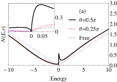
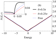
Figure 1: Total LDOS $N(E,r)=N_{reg}(E,r)+N_{\xi}(E,r)$ for $a=0.3,\mu=0.1,s=1$ and $r=0.3\;({\rm a}),r=1\;({\rm b})$; the insets are magnifications for $E\approx 0$. The free DOS for $a=0,\mu=0$ is included for comparison (dashed line).

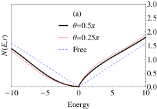
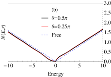
Figure 2: Total LDOS $N(E,r)=N_{reg}(E,r)+N_{\xi}(E,r)$ for $a=0.3,\mu=0.1,s=-1$ and $r=0.3\;({\rm a}),r=1\;({\rm b})$ The free DOS for $a=0,\mu=0$ is included for comparison (dashed line).

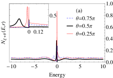
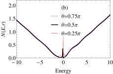
Figure 3: $N_{\xi+\theta}(E,r)=N_{\xi}(E,r)+N_{\theta}(E,r)$ with $l=0$ ($\gamma\approx 0.0035$) and $l=-1$; the inset is a magnification for $E\approx 0$ $({\rm a})$. Total LDOS $N(E,r)=N_{reg}(E,r)+N_{\xi}(E,r)+N_{\theta}(E,r)$ $({\rm b})$. On all panels: $a=0.59999$, $\mu=0.1$, $r=1$.

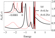
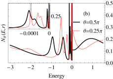
Figure 4: LDOS $N_{\theta}(E,r)$ with $l=-2,-1,0$ for $a=1.5,\mu=0.1$ ($\sigma\approx 0.539,1.446,1.375$) and $r=0.3\;({\rm a}),r=1\;({\rm b})$; the insets are magnifications for $E\approx 0$.

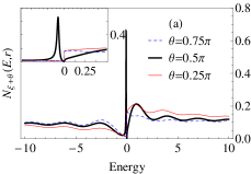
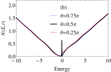
Figure 5: LDOS $N_{\xi+\theta}(E,r)=N_{\xi}(E,r)+N_{\theta}(E,r)$ for $l=0$ ($\gamma\approx 0.3162$) and $l=-1$ ($\sigma\approx 0.003$); the inset is a magnification for $E\approx 0$ $({\rm a})$. Total LDOS $N(E,r)=N_{reg}(E,r)+N_{\xi}(E,r)+N_{\theta}(E,r)$ $({\rm b})$. On all panels $a=0.45001$, $\mu=0.05$, $r=1$.

It should be commented: Since the summing range over $l$ for $s=-1$ is changed as compared to the one for $s=1$, little peaks in FIG. 2 absent. Families of the curves for the LDOS with $s=-1$ are qualitatively like to the ones given in FIGs. 3, 4 at the same values of $a,\mu,\xi,\theta$ except to the shift $l\to l+1$. Importantly, the LDOS exhibits resonances of the width $\sim|E_{k,\theta,s}|$ at the negative energies (49), which decay away from the impurity (see, FIG. 4 for $s=1$). Strong resonances appear in the vicinity of the Dirac point and signal the presence of the quasistationary states while at positive energies the LDOS exhibits periodically decaying oscillations (see, vpnn ; ashkl ). Increasing the effective charge will cause the resonances to migrate downwards in energy and their number to increase. This is because, in reality, the Dirac point is an accumulation point of infinitely many resonances vpnn .

FIG. 5 shows there is indeed the single resonance in the hole region when $\sigma\to 0$ at $\theta=\pi/2$ and only for $s=1$, which is in good accord with (49).

It should be noted that the local and total density of states in the pure Aharonov–Bohm potential with half-integers $\mu$ in graphene are calculated in ssladd . It was shown in ssladd that: 1) the peak of the LDOS, due to the divergent as $1/\sqrt{r}$ at the origin zero mode solution of the Dirac equation, should be observed at the Fermi level in graphene without gap in the quasiparticle spectrum; 2) when the energy is increased the LDOS very quickly reduces to the free density of states. These results can be obtained from Eqs. (51) and (53) putting in them $a=0,l=0,\mu=1/2$. Exact solutions to the Dirac equation in the pure Aharonov Bohm potential in 2+1 dimensions was found and discussed in khl10 for fermion bound states with the particle spin taken into account.

References

(1) K. S. Novoselov et al., Science, 306, 666 (2004).
(2) A.H. Castro Neto, F. Guinea, N.M. Peres, K.S. Novoselov,
and A.K. Geim, Rev. Mod. Phys., 81 109 (2009).
(3) V. N. Kotov, B. Uchoa, V. M. Pereira, F. Guinea and A. H. Castro Neto, Rev. Mod. Phys. 84, 1067 (2012).
(4) K.S. Novoselov et al, Nature, 438, 197 (2005).
(5) Z. Jiang, Y. Zhang, H.L. Stormer, and P. Kim,
Phys. Rev. Lett., 99 106802 (2007).
(6) V. M. Pereira, J. Nilsson, and A.H. Castro Neto,
Phys. Rev. Lett., 99 166802 (2007).