A Rank Minrelation - Majrelation Coefficient

Abstract

Improving the detection of relevant variables using a new bivariate measure could importantly impact variable selection and large network inference methods. In this paper, we propose a new statistical coefficient that we call the rank minrelation coefficient. We define a minrelation of $X$ to $Y$ (or equivalently a majrelation of $Y$ to $X$) as a measure that estimate $p(X\leq Y)$ when $X$ and $Y$ are continuous random variables. The approach is similar to Lin’s concordance coefficient that rather focuses on estimating $p(X=Y)$. In other words, if a variable $X$ exhibits a minrelation to $Y$ then, as $X$ increases, $Y$ is likely to increases too. However, on the contrary to concordance or correlation, the minrelation is not symmetric. More explicitly, if $X$ decreases, little can be said on $Y$ values (except that the uncertainty on $Y$ actually increases). In this paper, we formally define this new kind of bivariate dependencies and propose a new statistical coefficient in order to detect those dependencies. We show through several key examples that this new coefficient has many interesting properties in order to select relevant variables, in particular when compared to correlation.

1 Introduction

When it comes to selecting relevant variables (relevance as defined in (Kojadinovic, 2005)), many filter methods try to find the subset of variables ($X_{S}$) that is the most predictive to the target variable ($Y$) (Guyon & Elisseeff, 2003). Some of these efficient filter methods (such as ranking (Duch et al., 2003), mRMR (Peng et al., 2005), FCBF (Yu & Liu, 2004)) select a subset by identifying relevant variables based only on bivariate measures. However, the fact that the set $X_{S}$ is predictive to $Y$ do not ensure that its component variables $X_{i\in S}$ are relevant to $Y$ (Meyer et al., 2008). Improving the detection of relevant variables using a bivariate measure could importantly impact large network inference methods that rely heavily on bivariate measures (such as correlation networks (Butte & Kohane, 2000) or Aracne (Margolin et al., 2006)). The objective of this paper is precisely to define a new statistical coefficient that improves the detection of relevant variables using only a bivariate measure. We will see that our new coefficient implicitly focuses on the little studied issue of heteroscedasticity. Let us first provide some examples:

1. When the price of aluminum increases the prices of cars is likely to increase too. However, if the price of aluminum drops, the price of cars might stay high because of other components or some technological and economical considerations (i.e. other relevant variables). However, if the price of cars become really low, then it is likely that the price of their components, including aluminum, are considered as low too (i.e. relatively to their average values).

2. An increase in the level of adrenaline leads to an increased heart rate, but a low level of adrenaline do not prevent a high heart rate (because of other relevant variables) and a high heart rate do not mean a high adrenaline level. However, a low level of adrenaline is likely to be observed in a person having a low heart rate (w.r.t. to his/her usual heart rate).

3. Let $Y=X_{1}.X_{2}$ with $X_{1}\in[0,1]$, and $X_{2}\in[0,1]$. In such case, a low $X_{1}$ implies a low $Y$ but a high $X_{1}$ has little information on $Y$ (because a low $X_{2}$ automatically means a low $Y$ whatever the value of $X_{1}$). However, a high $Y$ (w.r.t. its average) automatically implies a high $X_{1}$.

In those examples, where variable dependencies are not quite correlations, looking for correlations might be fastidious because in order to observe joint variations, it might require that no other effect impacts the measured variables or that all those effects cancel each other. It worth noting that the joint distribution we are focusing on, illustrated by example 3 and also Fig. (1), has been identified in (D. Sahoo & Plevritis, 2008) as the distribution observed in variables exhibiting an implication relationship (a probabilistic version of it). However, (D. Sahoo & Plevritis, 2008) rely on discretization (in a maximum of three classes) to detect these dependencies whereas we will define a coefficient adapted to continuous variables, in Section 2. Assumptions will be discussed in 3. Properties of the new coefficient are stressed in Section4. In section 5, preliminary experiments show the competitivity of this new coefficient for variable selection w.r.t. correlation.

2 Minrelation

In this section, we will define the minrelation of $X$ to $Y$ as an estimate $\hat{p}(X\leq Y)$ of $p(X\leq Y)$ for continuous random variables.
Respectively, the majrelation of $X$ to $Y$ will be defined as the estimate $\hat{p}(X\geq Y)$ of $p(X\geq Y)$.

For example, let $m$ samples of $X\in[-0.5,0.5]$ and $Y\in[-0.5,0.5]$ be drawn such that $\forall(x_{i},y_{i}),x_{i}\leq y_{i},i\in\{1,...,m\}$, see Fig. (1). In such case, we say there is a perfect minrelation of $X$ to $Y$ (or equivalently a perfect majrelation of $Y$ to $X$), i.e. $\hat{p}(X\leq Y)=1$. In a linear model, the variance of $Y|X$ would decrease as $X$ increases and symmetrically, the variance of $X|Y$ decreases as $Y$ decreases. In other words, heteroscedasticity is a major component of a minrelation.

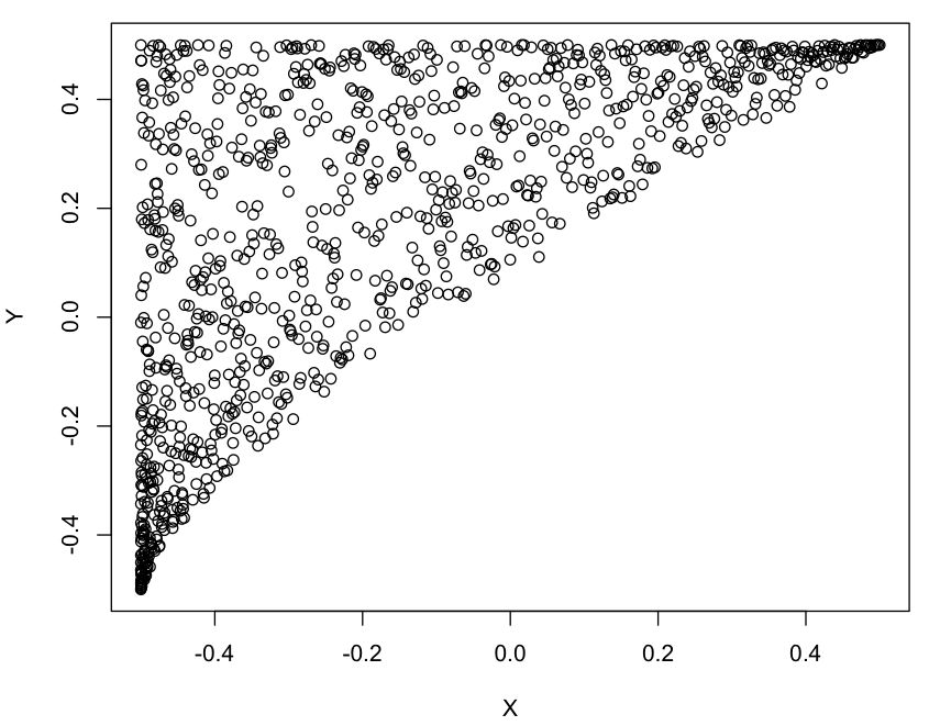
Figure 1: Typical plot of a minrelation between $X$ and $Y$. For a linear model, the variance of $Y|X$ decreases as $X$ increases and symmetrically the variance of $X|Y$ decreases as $Y$ decreases

Let us now relax the constraint and assume that $\exists j\in\{1,...,m\},x_{j}>y_{j}$. In that case, a simple way to estimate $p(X\leq Y)$ is to count the sample points $i$ that are concordant ($C$) with $x_{i}\leq y_{i}$,

$$\hat{p}(X\leq Y)=\frac{\sum_{i}I(x_{i}\leq y_{i})}{m}$$

with $I$ being the indicator function. Similarly, we can count the sample points that are discordant ($D$) with it:

$$\hat{p}(X\leq Y)=1-\frac{\sum_{i}I(x_{i}>y_{i})}{m}$$

In order to create a coefficient that range between -1 and +1, we can compute

$$\frac{C-D}{C+D}=\frac{\sum_{i}I(x_{i}\leq y_{i})-\sum_{i}I(x_{i}>y_{i})}{m}$$ (1)

The formula above focuses on the trade-off between $\hat{p}(X\leq Y)$ and $\hat{p}(Y\leq X)$. The problem with the proposed coefficient lies in the case where the joint distribution is symmetric. Ideally a high concordance (i.e. $\hat{p}(X=Y)$ close to 1) should lead to a high minrelation of $X$ to $Y$ (i.e. $\hat{p}(X\leq Y)$ close to 1) together with a high minrelation of $Y$ to $X$ (i.e. $\hat{p}(Y\leq X)$ close to 1). However, in this case, highly concordant variables and independent variables would both lead to a minrelation coefficient close to zero.

Note that there are four possible minrelations/majrelations

1. $\hat{p}(X\leq Y)$ equivalently $\hat{p}(-Y\leq-X)$

2. $\hat{p}(X\leq-Y)$ equivalently $\hat{p}(Y\leq-X)$

3. $\hat{p}(-X\leq Y)$ equivalently $\hat{p}(-Y\leq X)$

4. $\hat{p}(-X\leq-Y)$ equivalently $\hat{p}(Y\leq X)$

As a result, we rather propose another coefficient, that we denote by $\iota(X,Y)$, and which focuses on the trade-off between $\hat{p}(X\leq Y)$ and $\hat{p}(X\leq-Y)$, i.e.,

$$\iota(X,Y)=\frac{\sum_{i}I(x_{i}<-y_{i})-\sum_{i}I(x_{i}>y_{i})}{\sum_{i}I(x_{i}<-y_{i})+\sum_{i}I(x_{i}>y_{i})}$$ (2)

As a result, when the distribution is close to Fig. (1), $\iota$ is close to +1. However, when the distribution is close to Fig. (2), $\iota$ is close to -1.

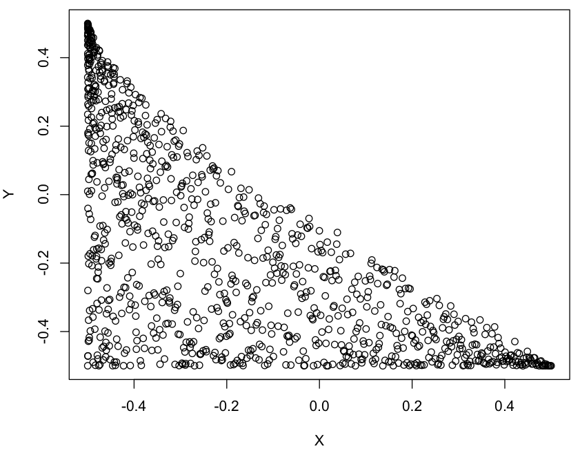
Figure 2: Typical plot of a minrelation between $X$ and $-Y$.

Although formula (2) can be applied to continuous random variables, it penalizes equally a point close to the diagonal $y=x$ and one far from it. Not only the agreement between which side of the diagonal falls each realization $(x_{i},y_{i})$, but the agreement between their relative distance to the diagonal, should matter. Hence, similarly to the concordance coefficient, we adopt here squared distance to the diagonal (Lin, 1989).

Hence, the higher the sum of the squared distances of the data points $i$ in discordance with the relation ($x_{i}\leq y_{i}$), the lower $\hat{p}(X\leq Y$). As a result, iota becomes

$$\frac{\sum_{i}I(x_{i}<-y_{i})(x_{i}+y_{i})^{2}-\sum_{i}I(x_{i}>y_{i})(x_{i}-y_{i})^{2}}{\sum_{i}I(x_{i}<-y_{i})(x_{i}+y_{i})^{2}+\sum_{i}I(x_{i}>y_{i})(x_{i}-y_{i})^{2}}$$ (3)

Although this formula looks less simple than the concordance coefficient, its computation is as straightforward.

3 Assumptions

We have implicitly assumed that $X$ and $Y$ are centered and normalized, but the question that arise now is: how should we center and normalize those variables? In other words, how can we compare variables with very different ranges of values (such as aluminum prices and car prices or adrenaline level and heart rate,…)?

The concordance coefficient applied to centered and normalized variables boils down to Pearson’s correlation. One strategy that has been adopted for normalizing variables in correlations consists in mapping marginals to ranks. For example, let

$$\bar{X}=\frac{r(X)}{m}$$ (4)

$$\bar{Y}=\frac{r(Y)}{m}$$ (5)

with $r$ the function that return the rank (in increasing order) of $x_{i}$ (resp. $y_{i}$) in the samples of $X$ (resp. in $Y$). In such case, where data are converted into ranks, the marginals are uniform distributions. As a result, when the concordance coefficient is applied on variable that have been first converted to ranks, it fits Spearman’s rank correlation.

However, a minrelation automatically implies that at least one marginal is asymmetric (unless in the particular case of a correlation). Obviously applying the minrelation coefficient on uniform distributions such as rank data will lead to wrong results because it is impossible to have $\forall i\in\{1,...,m\},\ r(x_{i})\leq r(y_{i})$ unless $\forall i\in\{1,...,m\},\ r(x_{i})=r(y_{i})$. Table (1) illustrates this phenomenon for binary variables where $p(x_{0},y_{1})>0$ automatically implies non-symmetrical marginals. In fact, both in Fig. (1) and in Table (1), we can see that the distribution of $X$ is a decreasing triangular distribution and that the distribution of $Y$ is increasing triangular.

$p(X\leq Y)$	$x_{0}$	$x_{1}$	$p(Y)$
$y_{0}$	0.33	0	0.33
$y_{1}$	0.33	0.33	0.66
$p(X)$	0.66	0.33	1

$p(X\leq-Y)$	$x_{0}$	$x_{1}$	$p(Y)$
$y_{0}$	0.33	0.33	0.66
$y_{1}$	0.33	0	0.33
$p(X)$	0.66	0.33	1

Table 1: Examples of minrelation between binary variables. The first table is analogous to Fig. (1) and the second one is analogous to Fig. (2).

Fortunately, we can map the data to a decreasing triangular distribution by weighting linearly the uniform distribution. In such case, the smallest rank should have the lowest weight and the highest rank should have the highest. In other words, the weight $w_{i}$ of each sample is precisely its ranking $r(x_{i})$.

This leads to

$$\grave{X}=\frac{r(X)^{2}}{m^{2}}-0.5$$ (6)

in order to have a centered decreasing triangular distribution, and

$$\acute{Y}=0.5-\frac{r(-Y)^{2}}{m^{2}}$$ (7)

in order to obtain an increasing triangular distribution (that mirrors $X$). Note that $r(-Y)$ is the ranks of $Y$ in decreasing order (instead of the increasing one).

This transformation not only map the range of values of $X$ and $Y$ to the interval $[-0.5,0.5]$ but also map $E[\grave{X}]$ to $-0.1666$ and $E[\acute{Y}]$ to 0.1666 that are precisely the values observed in the symmetric joint distribution illustrated in Table (1) and also in Fig. (1).

If we consider the estimation of $\hat{p}(X\leq-Y)$ (instead of $\hat{p}(X\leq Y)$, see Table (1)), we should rather use $\grave{Y}$ instead of $\acute{Y}$, in order to have a decreasing triangular distribution instead of an increasing one, with

$$\grave{Y}=\frac{r(Y)^{2}}{m^{2}}-0.5$$ (8)

Hence, we can define $\iota(X,Y)$, the rank minrelation coefficient, as the minrelation coefficient but applied on the variables converted to increasing (resp. decreasing) squared ranks. This is done by plugging $\grave{X}$, $\acute{Y}$ and $\grave{Y}$ in eq. 3. The rank minrelation coefficient $\iota(X,Y)$ becomes

$$\frac{\sum_{i}I(-\grave{x}_{i}<\grave{y}_{i})(\grave{x}_{i}+\grave{y}_{i})^{2}-\sum_{i}I(\grave{x}_{i}>\acute{y}_{i})(\grave{x}_{i}-\acute{y}_{i})^{2}}{\sum_{i}I(-\grave{x}_{i}<\grave{y}_{i})(\grave{x}_{i}+\grave{y}_{i})^{2}+\sum_{i}I(\grave{x}_{i}>\acute{y}_{i})(\grave{x}_{i}-\acute{y}_{i})^{2}}$$ (9)

4 Properties

This new coefficient benefits from the following properties

1. $-1\leq\iota(X,Y)\leq 1$

2. if $\forall(x_{i},y_{i}),x_{i}\leq y_{i}$ then $\iota(X,Y)=1$ (similarly if $\forall(x_{i},y_{i}),y_{i}\leq x_{i}$ then $\iota(Y,X)=1$)

3. if $X$ and $Y$ are independent, then $\iota(X,Y)=\iota(Y,X)=0$

4. if $\rho(X,Y)=1$ then $\iota(X,Y)=1$ and $\iota(Y,X)=1$

5. if $\rho(X,Y)=-1$ then $\iota(X,Y)=-1$ and $\iota(Y,X)=-1$

Hence, high correlation implies minrelated variables but high minrelations can happen with poorly correlated variables.
Moreover, thanks to the squared ranks conversion discussed earlier the joint distribution of $X$ and $Y$ becomes symmetric w.r.t. the diagonal $y=-x$, which leads to $\iota(X,Y)\simeq\iota(-Y,-X)$.
Obviously, there is a similar coefficient benefitting from the same properties: $\iota_{2}(X,Y)$ focusing on the trade-off between $\hat{p}(X\leq Y)$ and $\hat{p}(-X\leq Y)$ (instead of $\hat{p}(X\leq-Y)$).

In fact, $\iota(X,Y)=\iota_{2}(-Y,-X)$ and reciprocally $\iota_{2}(X,Y)=\iota(-Y,-X)$. Hence, $\iota(X,Y)$ and $\iota_{2}(X,Y)$ return close values once data have been converted to squared ranks.

However, if $X$ and $Y$ joint distribution is not symmetric w.r.t. the diagonal $y=-x$, these coefficients would actually answer different questions. For example, let us assume that increasing the dosage of a medication increases the probability of getting cured, i.e. $p(high\ dose,cured)$ is close to 1. In such case, $\iota(dose,cure)$ sort of compares $p(high\ dose,cured)$ with $\hat{p}(high\ dose,not\ cured)$ whereas $\iota_{2}(dose,cure)$ sort of compares $p(high\ dose,cured)$ with $\hat{p}(low\ dose,cured)$ (and hopefully $\iota_{2}<\iota$, being cured with a low dose is more likely than not being cured with a high dose).

5 Experiments

The goal of this section is to show the usefulness of the new rank minrelation coefficient $\iota$ in data analysis (when compared to Spearman’s $\rho$). We first demonstrate $\iota$ competitiveness on toy examples, then on artificial and real datasets by plugging it into the well-known ranking variable selection method (because it is based on pairwise similarity measure).

5.1 Multiplication

As mentioned in the introduction, one of the easiest way of generating minrelation consists in defining $B$ and $C$ as independent and uniformly distributed variables (in the positive range) and let $A=B.C$ because it results that $\hat{p}(A\leq B)=1$ and $\hat{p}(A\leq C)=1$ (after $A,B$ and $C$ are converted to squared ranks). We report in Table (2) the average value of minrelation and correlation coefficients over 1000 runs of the above setting where each variable is constituted of 1000 samples.

$X$	$A$	$A$	$B$
$Y$	$B$	$C$	$C$
$\rho(X,Y)$	0.66	0.66	0.00
$\iota(X,Y)=-\iota(X,-Y)$	0.99	0.99	0.00
$\iota(-Y,X)=-\iota(-Y,-X)$	-0.99	-0.99	0.00
$\iota(-X,Y)=-\iota(-X,-Y)$	-0.79	-0.79	0.00
$\iota(Y,X)=-\iota(Y,-X)$	0.77	0.77	0.00

Table 2: Correlation coefficient $\rho$ and minrelation coefficient $\iota$ where ($A,B$) and ($A,C$) have minrelation dependencies and ($B,C$) are independent (results are averaged over 1000 repetitions).

We observe that $\iota(X,Y)\simeq\iota(-Y,-X)$ and $\iota(Y,X)\simeq\iota(-X,-Y)$ exhibit quite close values as it is expected with the mapping of samples to squared ranks.

5.2 Linear dependencies

Let’s take another toy example with variables having linear dependencies. Let $A=3B+2C+D$ with $B$, $C$ and $D$ independent and normally distributed variables $N(0,1)$. The averaged results of 1000 runs with each variables having 1000 samples are reported in Table (3).

$X$	$A$	$A$	$A$
$Y$	$B$	$C$	$D$
$\rho(X,Y)$	0.79	0.52	0.26
$\iota(X,Y)$	0.98	0.81	0.46
$\iota(-Y,X)$	-0.98	-0.81	-0.46
$\iota(-X,Y)$	-0.98	-0.81	-0.46
$\iota(Y,X)$	0.98	0.81	0.46

Table 3: Correlation coefficient $\rho$ and minrelation coefficient $\iota$ where ($A,B$), ($A,C$) and ($A,D$) are all having a linear dependency (results are averaged over 1000 repetitions).

As expected, when the dependency between two variables is symmetric (i.e. in a linear setting), we observe close values for $\iota(X,Y)\simeq\iota(Y,X)$.

5.3 Multiplication together with linear dependencies

Let

$$\begin{array}[]{c}G=A+E\\ A=BCD\end{array}$$ (10)

and observe (in Table (4)) which of $G$ and the independent and uniformly distributed variables $B,C,D$ are more relevant in order to predict $A$ using both correlation and minrelation coefficients knowing that $E$ is a normally distributed variable $N(0,0.15)$ denoting the noise.

$X$	$A$	$A$	$A$	$A$	$A$
$Y$	$B$	$C$	$D$	$E$	$G$
$\rho(X,Y)$	0.53	0.53	0.53	0.00	0.57
$\rho(-X,Y)$	-0.53	-0.53	-0.53	0.00	-0.57
$\iota(X,Y)$	0.97	0.97	0.97	0.00	0.92
$\iota(-Y,X)$	-0.98	-0.98	-0.98	0.00	-0.87
$\iota(-X,Y)$	-0.69	-0.69	-0.69	0.00	-0.78
$\iota(Y,X)$	0.64	0.64	0.64	0.00	0.85

Table 4: Correlation coefficient $\rho$ and minrelation coefficient $\iota$ averaged over 1000 repetitions of the example given in Eq. (10).

Interestingly $\rho$ would rank variable $G$ first (higher correlation with $A$) whereas $\iota(X,Y)$ would rank it after $B,C,D$. However, if we look at $\iota(-X,Y)$ we can observe the same ranking than for $\rho$. The minrelation coefficient kind of splits the correlation signal into two parts: one coming from $(x_{i}\leq y_{i})$ and another coming from $(x_{i}\leq-y_{i})$. Hence, in the following, when we are not interested by the directionality of the minrelation, but rather by the ordering of relevance provided by each criterion (correlation vs minrelation), we will report $\rho^{2}$ and $\max\iota^{2}$ the maximum over the four possible values of $\iota$ (squared in order to avoid negative values).

5.4 Artificial dataset

The question that arise at this point is: is $\max\iota^{2}$ able to discriminate between relevant and irrelevant variables better than $\rho^{2}$? In order to answer this question, we make use of a synthetically generated dataset where relevant and irrelevant variables are known. In this experiment, we compare the performances of variables ranking by using $\rho^{2}$ and $\max\iota^{2}$ on our artificial datasets. We consider a ranking strategy superior if the average position of the relevant variables using that criterion is lower than for the other criterion. The rationale being that a better selection criterion should return a lower average position (i.e. relevant variables should be ranked first).

As artificial datasets, we adopt the 10 datasets of 100 variables coming from the DREAM4 challenge (i.e. KO1…KO5, MF1…MF5) where the goal was to identify predictor variables for each variables of the dataset (it is a network inference task) (Marbach et al., 2009). However, in this case, we focus only on the few variables per dataset that have more than 10 predictors. This minimal number of predictors ensure some stability in the results reported. Indeed, if one predictor variable happens to be badly ranked by chance there are at least 9 others that could compensate (if the criterion is indeed superior). The number of target variables (i.e. ranking tasks), wins and losses of each criterion for each dataset are reported in Table (5).

DATASET	targets	rank-$\rho^{2}$ wins	rank-$\iota^{2}$ wins
KO1	5	0	5
KO2	6	2	4
KO3	3	0	3
KO4	5	2	3
KO5	6	2	4
MF1	5	2	3
MF2	6	2	4
MF3	3	0	3
MF4	5	2	3
MF5	6	3	3
Tot	50	15	35

Table 5: Correlation coefficient $\rho^{2}$ vs minrelation coefficient $\max\iota^{2}$ in ranking strategies on target variables having more than 10 predictors in the 10 datasets of the DREAM4 competition. Column 1 indicates the dataset, column 2 indicates the number of variables having more than 10 predictors in that dataset and columns 3 and 4 reports the wins and losses of the two ranking methods on those target variables. A method wins if the average position of the predictors in the ranking is lower than for the other method.

We observe that $\max\iota^{2}$ exhibits results that are more than twice better than $\rho^{2}$ on a task that consists in identifying the known set of predictors of target variables in ten artificial datasets.

5.5 Real datasets

In the previous task, the variable to be selected were known in advance. It is usually not the case in real datasets. In order to compare $\rho$ and $\iota$ coefficients on real data, we evaluate the prediction accuracy of different learning algorithms (i.e. linear model, random forest and radial SVM) using as input variables the best ranked ones using $\rho^{2}$ and $\max\iota^{2}$. We assume here that a better criterion leads to a better ranking of variables which in turn leads to better prediction performances of a model built on these top ranked variables. We carried out an experimental session based on four regression datasets publicly available (Torgo, ). For computational reasons, we have limited the number of samples per dataset to 600 (randomly sampled). The name of the datasets together with the number of variables and number of samples are reported in Table (6).

dataset	name	$n$	$m$
1	Ailerons	35	600
2	Pol	26	600
3	Triazines	58	186
4	Wisconsin	32	194

Table 6: Regression datasets, together with their number of variables $n$ and number of samples $m$, used as benchmark.

In order to eliminate a possible variable selection bias, each dataset is first divided into two equal parts, one for ranking variables and one for evaluating those rankings. The evaluation of a ranking method is given by the mean squared error returned by a 10-fold cross-validation of a linear regression (R lm function), a SVM with radial kernel (R package e1071) and a random forest (R package randomForest). In order to avoid the bias related to the size of the feature set, we average the performance over all the feature sets size (that range from 2 to 10 for each dataset) (Bontempi & Meyer, 2010). Table (7) reports the wins and losses on the four datasets for each learning algorithm as well as per datasets.

rank-$\iota^{2}$ vs rank-$\rho^{2}$	wins	loss
Linear model	2	2
Random forest	2	2
SVM radial	2	2
total	6	6

rank-$\max\iota^{2}$ vs rank-$\rho^{2}$	wins	loss
Ailerons	0	3
Pol	0	3
Triazines	3	0
Wisconsin	3	0

Table 7: Comparison of ranking strategies based on $\rho^{2}(X,Y)$ and $\max\iota^{2}(X,Y)$. Wins and losses are defined by the lower 10-fold-cross-validated mean squared error returned by a linear regression, a radial SVM and a random forest averaged over subset sizes ranging from 2 to 10, for each of the four datasets.

We observe here that $\max\iota^{2}$ outperform $\rho^{2}$ on two datasets and underperform $\rho^{2}$ on the two others, those results are independent of the learning strategy used.

6 Conclusion

The goal of this paper has been to introduce a new measure of bivariate dependency called a minrelation. We defined a new statistical rank coefficient to determine if two continuous variables are minrelated (or respectively majrelated). Finally, we showed the usefulness of the minrelation coefficient on toy examples as well as on artificial and real datasets. Indeed, $\max\iota^{2}$ appears to be a competitive criterion w.r.t. Spearman’s $\rho^{2}$ for ranking variables. We deem that competitive results with Spearman’s correlation makes this coefficient an appealing new tool for the toolbox of any data analyst. Furthermore, we believe that specific selection strategies that take into account the directionality of the minrelation will hold bigger promises. However, further research should focus on that topic as well as on the limitations of this new measure (i.e. sample statistic, linearity assumptions or even spurious case of high iota values).

References

- Bontempi & Meyer (2010) Bontempi, G. and Meyer, P. E. Causal filter selection in microarray data. In International Conference On Machine Learning (ICML), 2010.
- Butte & Kohane (2000) Butte, A. J. and Kohane, I. S. Mutual information relevance networks: Functional genomic clustering using pairwise entropy measurments. Pacific Symposium on Biocomputing, 5:415–426, 2000.
- D. Sahoo & Plevritis (2008) D. Sahoo, D. L. Dill, A. J. Gentles R. Tibshirani and Plevritis, S. K. Boolean implication networks derived from large scale, whole genome microarray datasets. Genome Biology, 2008.
- Duch et al. (2003) Duch, W., Winiarski, T., Biesiada, J., and Kachel, A. Feature selection and ranking filters. In International Conference on Artificial Neural Networks (ICANN) and International Conference on Neural Information Processing (ICONIP), pp. 251–254, June 2003.
- Guyon & Elisseeff (2003) Guyon, I. and Elisseeff, A. An introduction to variable and feature selection. Journal of Machine Learning Research, 3:1157–1182, 2003.
- Kojadinovic (2005) Kojadinovic, I. Relevance measures for subset variable selection in regression problems based on k-additive mutual information. Computational Statistics and Data Analysis, 49, 2005.
- Lin (1989) Lin, L I-K. A concordance correlation coefficient to evaluate reproducibility. Biometrics, 1989.
- Marbach et al. (2009) Marbach, D., Schaffter, T., Mattiussi, C., and Floreano, D. Generating realistic in silico gene networks for performance assessment of reverse engineering methods. Journal of Computational Biology, 2009.
- Margolin et al. (2006) Margolin, A. A., Nemenman, I., Basso, K., Wiggins, C., Stolovitzky, G., Favera, R. Dalla, and Califano, A. ARACNE: an algorithm for the reconstruction of gene regulatory networks in a mammalian cellular context. BMC Bioinformatics, 7, 2006.
- Meyer et al. (2008) Meyer, P. E., Schretter, C., and Bontempi, G. Information-theoretic feature selection using variable complementarity. IEEE Journal of Special Topics in Signal Processing, 2(3), 2008.
- Peng et al. (2005) Peng, H., Long, F., and Ding, C. Feature selection based on mutual information: criteria of max-dependency, max-relevance, and min-redundancy. IEEE Transactions on Pattern Analysis and Machine Intelligence, 27(8):1226–1238, 2005.
- (12) Torgo, L. URL http://www.liaad.up.pt/~ltorgo/Regression/DataSets.html.
- Yu & Liu (2004) Yu, L. and Liu, H. Efficient feature selection via analysis of relevance and redundancy. Journal of Machine Learning Research, 5:1205–1224, 2004.