Bulk asymptotics for polyanalytic correlation kernels
Abstract.
For a weight function and a positive scaling parameter , we study reproducing kernels of the polynomial spaces
equipped with the inner product from the space . Here denotes a suitably normalized area measure on . For a point belonging to the interior of certain compact set and satisfying , we define the rescaled coordinates
The following universality result is proved in the case :
as while for any fixed , uniformly for in compact subsets of . The notation stands for the associated Laguerre polynomial with parameter and degree . This generalizes a result of Ameur, Hedenmalm and Makarov concerning analytic polynomials to bianalytic polynomials. We also discuss how to generalize the result to . Our methods include a simplification of a Bergman kernel expansion algorithm of Berman, Berndtsson and Sjöstrand in the one compex variable setting, and extension to the context of polyanalytic functions. We also study off-diagonal behaviour of the kernels .
Key words and phrases:
Polyanalytic function, determinantal point process, Landau level, Bergman kernel1. Introduction
1.1. Notation
We will write and for the boundary and the interior of a subset of the complex plane . By we mean the characteristic function of the set . We let
be the normalized area measure in , and use the standard Wirtinger derivatives
Will will often omit the subscripts if there is no risk of confusion. We write , and it can be observed that this equals to one quarter of the usual Laplacian. We write for the open unit disk, and more generally for the disk with center and radius . Given a Lebesgue measurable function , we denote by the space of measurable functions which are square-integrable with respect to the measure .
1.2. Spaces of polyanalytic polynomials
Let be a continuous function satisfying
| (1.1) |
for two positive numbers and . This function will be referred to as the weight. We set
and
The space is a finite dimensional, and thus closed, subspace of . We see that when , the growth condition on implies that contains the whole .
Notice that consists of analytic polynomials of degree at most . For a more general , functions in the spaces will be called -analytic polynomials.
By a -analytic function, we mean a continuous function that satisfies the equation in the sense of distribution theory. A function which is -analytic for some is called polyanalytic. Obviously, -analytic polynomials form a subclass of -analytic functions. It is also easy to see that a -analytic function can be written as
| (1.2) |
for some analytic functions . The decomposition provides a correspondance between -analytic functions and vector-valued analytic functions; this connection is explained in [22] in more detail.
The space possesses the reproducing kernel
where is any orthonormal basis for . It is well-known that does not depend on the choice of the basis and that the reproducing property
holds for all .
1.3. Determinantal point processes
Assuming , which implies that is -dimensional, we use to define the following probability distribution on :
| (1.3) |
where
| (1.4) |
This is a particular instance of a so called determinantal point process. That is a probability measure follows from standard arguments (see any book on random matrices, e.g., [17], [29]); this depends only on the fact that is a kernel of a projection to a -dimensional subspace of . It is customary to identify all the copies of the complex plane and permutations of the points , and think the process as a random configuration of unlabelled points in .
For , let us define the -point intensity functions by
It is a well-known fact about determinantal point processes that all the intensity functions are easily expressed with the kernel :
The one-point intensity is particularly important, since integrating it over a set gives the expected number of points in .
The intensity functions are often called correlation functions in the literature, and the weighted kernel is referred to as the correlation kernel of the process.
1.4. Weighted potential theory
To discuss previous results on analytic polynomial kernels, we need to recall some facts from weighted potential theory. Let us assume that the weight is -regular in and satisfies the growth condition (1.1). We define and to be the sets
The equilibrium weight is defined as the largest subharmonic function in which is everywhere and has the growth bound
| (1.5) |
The function is then subharmonic and it follows from general theory for obstacle problems that it is regular (see [19]). There is also an elementary proof of this fact due to Berman [7]. The coincidence set of the obstacle problem is
This is a compact set and because is subharmonic, we have . It is known that is harmonic on . The set is a central object in weighted potential theory as it arises as the support of the unique solution to the energy minimization problem
where
| (1.6) |
The infimum is taken over all compactly supported Borel probability measures. Existence and uniqueness in this problem is due to Frostman. For more details, see [33]. Note that the functional (1.6) coincides with the standard logarithmic energy in the special case . The solution to energy minimization problem can be written as (see [19] or the earlier preprint [18])
| (1.7) |
The measure will be referred to as the equilibrium measure.
1.5. Bergman kernels for analytic polynomials
Kernels and associated probability densities were studied by Ameur, Hedenmalm and Makarov in [3], [4] and [5]. There are three possible interpretations for these point processes: in terms of Coulomb gas, free fermions or eigenvalues of random normal matrices. For more details, we refer the reader to [37].
As while , Hedenmalm and Makarov ([18], [19]) showed, building on the work of Johansson [24], that
| (1.8) |
in the weak-* sense of measures for all fixed .111This result is just a special case of their theorem, which holds for Coulomb gas models in arbitrary temperatures. Here, the notation stands for the ’th tensor power of the measure . As the authors showed in [19], this result can be used to show that for any bounded continuous function , we have the convergence
| (1.9) |
in distribution. Recalling (1.7), the intuitive interpretation of this is that the points from the determinantal process defined via tend to accumulate on with density as while . The set was called droplet for this reason.
Let us write bulk for the interior of the set . The results of [4] show that for a bulk point and a -tuple picked from the density
the local blow-up process at with coordinates
converges to the Ginibre process, as while . If we write for the -point intensity of the blow-up process, this means that
| (1.10) |
as while , for all and . Notice that the kernel appearing in the determinant on the right hand side is the reproducing kernel of the Bargmann-Fock space.
This fact could be interpreted as a universality result in the spirit of random matrix theory and related fields. In general, universality means that there exists a scaling limit which does not depend on particularities of the model (see [14] for more discussion). In our setting, this is reflected by the fact that the the limiting process is the same for all weights .
One can also formulate a universality result more directly in terms of the kernel . To do this, let us define the Berezin density centered at as
The main theorem in [3] was as follows:
Theorem 1.1 (Ameur, Hedenmalm, Makarov).
Fix and suppose that is real-analytic in some neighborhood of . Then
where the convergence holds in .
It should be mentioned that Berman [8] proved a similar result independently, also in a higher-dimensional setting.
Our main result will be a generalization of a slight reformulation of theorem 1.1 to the context of more general polyanalytic polynomial kernels .
1.6. Polyanalytic Ginibre ensembles
In a joint paper with Hedenmalm [21], we studied kernels with the weight and called the associated determinantal point processes Polyanalytic Ginibre ensembles. As we explained in this paper, these point processes describe systems of free (i.e. non-interacting) electrons in in a constant magnetic field of strength perpendicular to the plane, so that each of the first Landau levels contains particles. This model has also been studied in physics literature, see Dunne [15].
The analysis was in terms of the Berezin density, which was defined as in the case :
In the macroscopic lenght scales, we showed that,
as while . Here stands for the Dirac point mass at and for the harmonic measure at with respect to the domain . Notice that both limits are clearly independent of .
For microscopic length scales in the bulk , we obtained
| (1.11) |
where is the associated Laguerre polynomial with parameter and degree .
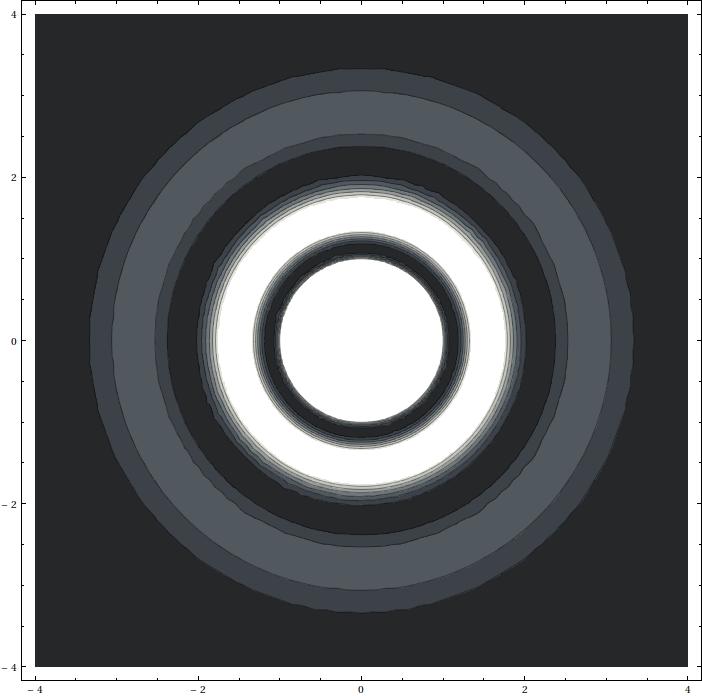
It might be interesting to recall that the Laguerre polynomial has zeros on the positive real axis. In terms of the points process, this means that around each point from the process, there are rings around , the radii of which are of the order of magnitude , so that there is no repulsion between and points on those rings in the limit as . So, one would expect the electrons to accumulate on those circles around any given electron. It should be emphasized that this phenomenon is not present in the analytic case .
We want to mention here that in [21], we also studied the Berezin kernels near the edge . We will not discuss such issues in this paper, and will only refer the interested reader to the original article.
1.7. Main results
Our aim is to generalize the results from polyanalytic Ginibre ensembles to more general weights . For simplicity, we mostly work with , but the proof methods should work for any . We start by analyzing the one point function . In section 3, it is shown in that this expression tends to zero for in an exponential rate as . This means that the points tend to accumulate on as in the analytic case .
Within , the following theorem presents more detailed information. It states that the bulk scaling limits obtained for polyanalytic Ginibre ensembles are universal.
Theorem 1.2.
Set . Fix and . Assume that is -smooth, satisfies the growth condition (1.1) and is real-analytic in a neighborhood of . Then, there exists a number such that for all , we have
| (1.12) |
as and . The convergence is uniform on compact sets of .
One can check that with the weight , the theorem is a slight reformulation of (1.11).
Basic structure of our argument will be the same as in [3]. There, the authors relied on two main techniques: algorithm of Berman-Berndtsson-Sjöstrand [9] to compute asymptotic expansions for Bergman kernels, and Hörmander’s -estimates. First, we will simplify the method of Berman-Berndtsson-Sjöstrand (in the one complex variable context only) and then extend it to polyanalytic functions. In a joint paper with Hedenmalm [22], we already showed how to obtain asymptotic expansions in the polyanalytic setting, but the approach we will take here will be more elementary and also computationally simpler.
Whereas in [3] certain estimates for the -operator are used, we need similar results for the operators with . As a consequence, we also obtain an off-diagonal decay estimate for bianalytic Bergman kernels, which, informally speaking, says that correlations are short range in . Comparing with the similar result in [3], one sees that the decay is essentially as strong as in the case . Again, we present a proof for the case , but the method should generalize to any .
Theorem 1.3.
Suppose that is -smooth. Fix a compact set in the interior of and constant . Set
Then, there exist positive constants and such that for any and , it holds
where we assume and . The constants and only depend on and .
One can of course ask what happens if the point is allowed to be outside . The answer will be provided in section 3, where we show that even stronger decay holds as .
It is possible that this off-diagonal decay estimate, or a variant of it, could also be used in other contexts to extend known results about analytic functions to polyanalytic functions. We should mention at least the work of Ortega-Cerdà and Ameur [6] concerning Fekete points as well as that of Ortega-Cerdà and Seip [32] on description of sampling and interpolation sets. The latter topic in spaces of polyanalytic functions is related to time frequency analysis (see Abreu [1]).
It would also be natural to study asymptotics of near the edge of the droplet but this question remains open even in the case .
1.8. Further questions: letting tend to infinity
It is also possible to let all the parameters and tend to infinity in our model. We explained already in [21] that the rescaled Berezin transform
converges to the limit if we first let while and then let afterwards. Here, is the standard Bessel function. Because of theorem 1.2, a similar result also holds when the weight is more general. Interestingly, this Bessel kernel could be viewed as a two-dimensional analogue of the sine kernel from Hermitian random matrix theory: the latter is the Fourier transform of a charateristic function of an interval while the former is the Fourier transform of a characteristic function of a disk.
It would interesting to study the asymptotics for as and go tend to infinity simultaneously. To get a very symmetric model, one could set , require that and then let tend to infinity. It seems likely that the above Bessel kernel would also arise here in the limit.
1.9. Further questions: fluctuations
In [4] and [5], fluctuation field of the random normal matrix model was shown to converge to Gaussian free field, in the first paper with the restriction that the test function is supported in the interior of . The methods of the first paper should apply to the polyanalytic setting, given the technology we develop in the present paper. The argument of [5], where the case of more general test functions was treated using so called Ward identities, seems harder to generalize.
2. Construction of local polyanalytic Bergman kernels
In this section, we present an algorithm to compute asymptotic expansions for polyanalytic Bergman kernels near the diagonal. For analytic functions, this is a well-studied topic in several complex variables literature see e.g. [11], [38], [34], [31]. The algorithm we present here is based on the work of Berman, Berndtsson and Sjöstrand [9], whose method relies on a certain technique from microlocal analysis (for an detailed exposition in the one complex variables setting, see [3]). Here we will show that at least in the one-dimensional case, this technique can be dispensed with. In particular, we get an alternative way to obtain results of Ameur, Hedenmalm and Makarov in the case . We then show how to extend this modified algorithm to polyanalytic functions. This provides a simplification of the method of [22], which was based on the original microlocal analysis technique.
We take an arbitrary and assume that is real-analytic in a neighborhood of . We will also pick such that the following conditions are satisfied:
-
(1)
is real-analytic in and on .
-
(2)
There exists a local polarization of in , i.e. a function which is analytic in the first and anti-analytic in the second variable, and satisfies .
-
(3)
For , we have and ; these conditions are made possible by condition . Here is the phase function which is defined below.
- (4)
We define the phase function as
Notice that is analytic in the first variable and real-analytic in the second. It can be analytically continued to the diagonal, and we have . More generally,
| (2.3) |
This leads to the following Taylor expansion, which we will need repeatedly:
| (2.4) |
where
We fix to be a smooth and non-negative cut-off function which equals on the interval and is supported on . We then define ; this function will then be supported on and equal on .
We will write for the subspace of -analytic functions in :
| (2.5) |
Clearly, the spaces are closed subspaces of . We will use the notation for the norm in the spaces , and .
We start by proving a lemma that will be frequently used in the sequel.
Lemma 2.1.
Let and be -analytic in the first variable and real-analytic in the second. We also assume that there exists and a positive integer such that
for all and . Then, given integers and satisfying and , there exists such that
| (2.6) |
for any and . The number and the constant of the error term are independent of and .
Proof.
Let us start with . By (2.2), we have
| (2.7) |
for some positive constants and . This shows the desired statement for the case .
For , we integrate by parts:
| (2.8) |
The statement follows after carrying out the differentiation and analyzing each term in the resulting sum as in the case . ∎
Next, we will prove an approximate reproducing identity for polyanalytic functions. For the case , this was already done in [22]. Here we present the argument for general .
Proposition 2.2.
There exists , independent of , such that for all and , we have
| (2.9) |
where
| (2.10) |
The constant of the error term in (2.9) is independent of and .
Proof.
We will use the fundamental solution of the operator (recall that our reference measure is the usual area measure divided by , so there is no need for that normalization here). Because of lemma 2.1 and -analyticity of , we have
| (2.11) |
for some .
Denoting by the Dirac point mass at , we get
| (2.12) |
where
| (2.13) |
Applying Leibniz rule in the sense of distribution theory shows that
| (2.14) |
So actually, the singularity in (2.13) cancels and is -analytic in and real-analytic in . ∎
A function which is -analytic in the first variable and real-analytic in the second will be called a local -analytic reproducing kernel if for any and , we have
| (2.15) |
where the constant of the error term can depend on , and but not on and . Clearly, proposition 2.2 shows that satisfies this condition. We define a local reproducing kernel similarly, just by replacing the factor in the error term by . If a local reproducing kernel with any error term is -analytic in (i.e. satisfies ), it will be called a local -analytic Bergman kernel.
In [22], we presented an algorithm producing local -analytic Bergman kernels for arbitrary , based on a microlocal analysis technique of Berman-Berndtsson-Sjöstrand [9] in the analytic case . We will next show that when , Taylor expansion and partial integration is enough. After this we show in the case , how this approach can be extended to more general polyanalytic functions. Later, in section 5, we will show that when , local bianalytic Bergman kernels actually provide a near-diagonal approximation of the kernel as .
2.1. Computation of local analytic Bergman kernels
The aim is to show how to compute local analytic Bergman kernels in the form
| (2.16) |
where all the coefficient functions 1,j are analytic in and . We denote by a function on which is analytic in and real-analytic in but whose exact form is not of interest to us. The number will denote a positive number that can change at each step.
Let and . We check from (2.10) that
| (2.17) |
Then, recalling proposition 2.2 and the Taylor expansion 2.4, we compute
| (2.18) |
where for the last equality, we needed an application of lemma 2.1. Here and later in computations of this nature, the choice of and the error constant is independent of , and .
We Taylor expand using (2.4), and continue the analysis:
| (2.19) |
For the third equality, lemma 2.1 was again used. The fact that we get a factor in last error term is a consequence of a small computation which we include here for the convenience of the reader. Let be -smooth and assume
for a constant . Then, using (2.2) and Cauchy-Schwarz inequality,
| (2.20) |
The conclusion is that
is a local analytic Bergman kernel . It is possible to continue in the same way and compute local Bergman kernels for any positive integer ; in order to do this, one just has to use higher order Taylor expansions of . Notice that the local Bergman kernels provided by this process are indeed conjugate analytic in ; this follows from the fact that the coefficient functions in the Taylor expansion (2.4) have this property.
Remark 2.3.
In the computation of local Bergman kernels, we do not necessarily need to require that : it is enough to assume that is analytic in and then replace by in the error terms.
2.2. Local bianalytic Bergman kernels
We will now explain how to extend the above method to a more general polyanalytic setting. We focus on the case . The functions satisfying will be called bianalytic. The intention is to show how to compute local bianalytic Bergman kernels in the form
| (2.21) |
where and all the coefficient functions are bianalytic in and .
Proceeding as in the case , we will expand the kernel in powers of so that the coefficients are bianalytic in . The following proposition will replace the partial integration that was performed in the analytic setting.
Proposition 2.4.
Let be a -smooth function. Then, there exists such that for any and , we have
| (2.22) |
The constant of the error term is independent of , and .
Proof.
The proof involves only partial integration.
| (2.23) |
where we used lemma 2.1 to get the last equality.
We leave the first integral in the last expression of (2.23) as such and continue with the analysis of the second.
| (2.24) |
where the third and the fifth equality depended on lemma 2.1. After carrying out the differentiations in the last integrand, the assertion follows from combining (2.23) with (2.24). ∎
We will now illustrate how the result can be used by computing two first terms of the expansion (2.21). We let stand for a function defined on which is bianalytic in the first variable and real-analytic in the second.
We see from (2.10) that
| (2.25) |
By Taylor expanding this expression with (2.4), we get
| (2.26) |
We require the coefficients in (2.21) to be bianalytic in and , which means in particular that they may not contain the factor to any degree higher than . Only the last three terms in (2.26) contain , so they are the only ones which require further analysis. For the term with , proposition 2.4 shows that
| (2.27) |
As we are only interested in the coefficients for and , we conclude that this term is negligible for our purposes. Note that the extra factor in the error term comes from the computation similar to (2.20). For the term with , two applications of proposition 2.4 are needed to show this:
| (2.28) |
We now set
and analyze the corresponding term in (2.26) with the proposition 2.4.
| (2.29) |
where
| (2.30) |
We expand in powers in :
| (2.31) |
We implement this into (2.29) and see by the same argument as in (2.27) that the term with is negligible We now put everything together within (2.26):
| (2.32) |
where
| (2.33) |
and
| (2.34) |
We conclude that
| (2.35) |
is a local bianalytic Bergman kernel .
We have also computed the third term:
| (2.36) |
where
| (2.37) |
The rather long computations are presented in the appendix.
3. Some estimates for the one-point function
In this section, we provide an apriori bound for the one point function
for and show that for we have convergence to zero with a rate that is exponential in .
In [3], analogous results were shown for kernels relying heavily on the fact that is subharmonic whenever is an analytic function. This is no longer true when is more general polyanalytic function, so we must use a different strategy.
Let us recall the following result, which is just proposition 8.1 of [22] in slightly altered form. Later, in lemma 4.2, we will show how a more general version of this result follows from proposition 4.1 of that paper.
Lemma 3.1.
For any bianalytic function and , we have
| (3.1) |
and
| (3.2) |
where
As an implication, we get two useful estimates for the kernel . Namely, taking for some fixed and using
we get the following estimate for the one-point function on :
| (3.3) |
where
Combining (3.3) with Cauchy-Schwarz inequality gives
| (3.4) |
We now apply the lemma 3.1 to provide an analogue of lemma 3.5 in [3]. We will need a simple weighted maximum principle for analytic polynomials provided by lemma 3.4 of the same paper (see also theorem III.2.1 in [33]). The proof is based on using the definition of and an application of maximum principle.
Lemma 3.2.
Suppose and . Let be an analytic polynomial of degree satisfying
Then
Proposition 3.3.
Suppose and . Then, there exists a constant depending only on such that for all and , it holds
Proof.
We take which minimizes the quantity
Let be the value of this expression corresponding to the optimal choice of . We write for analytic and . According to (3.2),
and
| (3.5) |
where
We can now apply lemma 3.2 to get
| (3.6) |
and
| (3.7) |
The statement of the proposition follows from putting (3.6) and (3.7) together:
| (3.8) |
where the constant only depends on and . ∎
From this result, we deduce
| (3.9) |
and because
we get
| (3.10) |
for all . Notice that this estimate is only interesting for , because for , we already have a better estimate in (3.3). We conclude that the one-point function decays exponentially to zero for a fixed as . Moreover, the growth conditions (1.1) and (1.5) imply that for any neighborhood of , we have
Finally, we want to record the the following off-diagonal analogue of (3.10):
| (3.11) |
In particular, for fixed and , we have again exponential decay to whenever one of the two points is in . This should be compared with the off-diagonal damping theorem 1.3, which deals with the case when both and belong to .
4. Hörmander-type estimates for
The purpose of this section is to prove theorem 4.5, which is an estimate for a solution of the equation , where a certain growth condition is imposed on the solution near infinity. This result will be used in section 6 to prove an off-diagonal decay estimate for bianalytic Bergman kernels.
We will assume that . We can always arrange this by adding a sufficiently big constant to . This just means that the corresponding reproducing kernel will be multiplied by a constant and so the problem remains essentially unchanged.
We start by fixing and setting
We have ; this is because is strictly subharmonic in the interior of . We choose two positive numbers and so that
| (4.1) |
this is possible because of the assumption and the growth condition
Notice that this implies immediately . We will also need to assume that .
We define
The definitions are exactly as in [3]. Intuitively, we would like to think to be equal to ; it however turns out that two correction terms involving the constants and are needed. The purpose of the logarithmic correction term is that now the weight becomes strictly subharmonic in the whole plane:
| (4.2) |
for a.e. and . The effect of substracting the term is
| (4.3) |
We also see that
| (4.4) |
on .
We fix and suppose that . We will work with a function which is -smooth on , zero on , constant on and satisfies the properties
| (4.5) | |||
| (4.6) | |||
| (4.7) |
for . The role of these conditions will become clear in the proof of theorem 4.5. A consequence of the estimate (4.5) is that
| (4.8) |
for a.e. . We also have
| (4.9) |
for a.e. .
Our argument is based on iterating the elementary one-dimensional version of Hörmander’s -estimate. This result states that for and satisfying a.e., there exists a solution to the equation
| (4.10) |
satisfying
provided that the right hand side is finite. It is also known that there exists a unique norm-minimal solution to (4.10). Namely, given any solution to the equation, can be written as
where denotes the projection to the subspace of analytic functions within .
Theorem 4.1.
Let be supported on and let satisfy the conditions above. Then, there exists a solution to the equation
satisfying
| (4.11) |
for all , where is a positive constant depending only on the parameters , and .
Proof.
Let us consider the equation
where is some function to be specified in a moment.
According to Hörmander’s result and (4.9), there exists a solution to the equation with the norm control
| (4.12) |
We would like to proceed by using Hörmander’s estimate again with the weight . But this is not possible, because the function is not -smooth. We proceed by replacing it with another function which is smooth enough. Building on (4.8) and (4.9), we estimate
where is any -smooth function satisfying
and
for . It will be convenient to make the change of variables , so that we can rewrite
We define another function by , and set
and
It remains to define on the interval . We set
where
The motivation for the definition of is that it solves the equation . We are here assuming that , where is so large that
and for all such . Notice that this definition of implies that on the annulus we have
For the remaining interval , the choice of is rather insignifigant. We can namely choose any decreasing function so that the resulting function defined on the whole real line becomes and whose second derivative is not smaller than .
With this construction of , we now see from (4.8) and (4.9) that
for and
for . In any case, is strictly subharmonic a.e. in the whole complex plane (we use here the assumption from the beginning of this section).
We can now apply Hörmander’s estimate the second time. We take to be thel solution of
which is norm-minimal in . We can now continue from (4.12):
| (4.13) |
and the proof is complete. ∎
We will now prove a generalization of lemma 3.1.
Lemma 4.2.
Take , and let be a -smooth real-valued function on . Then, for any bianalytic function , we have
| (4.14) |
and
| (4.15) |
where
Proof.
We assume without loss of generality. In [22], it was proved that for a bianalytic function on and a subharmonic function satisfying
it holds
| (4.16) |
where denotes the Green’s potential of the measure :
We will set and for . We have and
An application of (4.16) gives
| (4.17) |
which proves the first inequality. The second inequality follows the same way from
| (4.18) |
which also was proved in [22]. ∎
In the following lemma and later, we will use the notation for the largest integer smaller than or equal to a real number .
Lemma 4.3.
Let and be analytic functions, and suppose that
Then, and are polynomials of degree .
Proof.
From lemma 4.2, we get
where
Using (4.2), we see that
| (4.19) |
where
The last equality followed from harmonicity of in . By (4.19), we have
for all . This, together with the growth condition
| (4.20) |
shows that is a polynomial of degree . For , we first estimate
We use (4.14) with for the first term:
We get
| (4.21) |
The desired assertion for now follows from the growth condition (4.20) and that is a polynomial of degree ∎
We now turn to a definition of certain subspaces of , where is some real-valued -smooth weight function on . We assume that so that all constant functions belong to the space. Let us first fix some notation:
and
The spaces in question are
| (4.22) |
We see immediately that these spaces are not in general closed in . An important fact however is that
| (4.23) |
and is always closed in . This makes it possible to speak about -minimal solutions to -equations.
We will make use of the fundamental solution of the operator and denote the associated solution operator by :
for a compactly supported -function . We also write for the orthogonal projection from to .
Because , we have by (4.23) that
is the unique -minimal solution to the equation
This solution is characterized among the solutions in the class by the condition
which should hold for all .
The following lemma is an adaption of lemma 4.2 in [3] to our bianalytic context.
Lemma 4.4.
For any compactly supported function , the equation
has a solution in . The -minimal solution is of class when .
Proof.
The function solves the equation and satisfies as . Therefore, it belongs to the class . The -minimal solution can be written as
for some bianalytic function . Because we assume that is -smooth and constant in , the spaces and equal as sets, and therefore, by (4.3) and lemma 4.3, we get the inclusion
Hence, , and also . Because is bounded and as , we see that . The assertion is now proved. ∎
Theorem 4.5.
Fix a number such that and let be supported on and equal to on . Assume
where is as in proposition 4.1. Let be a -smooth function which is supported on , zero on and satisfies the conditions (4.5), (4.6) and (4.7). Then, the -minimal solution to the equation satisfies
| (4.24) |
In the special case , the conditions and on are not needed.
Proof.
The norm-minimality condition for can be rephrased as
| (4.25) |
This is because and are equal as sets. Because is supported on a compact set, we have . Therefore, is the -minimal solution to the equation
| (4.26) |
Let be the -minimal solution of the problem (4.26), the existence of which is guaranteed by lemma 4.4. We deduce from the same lemma that , and consequently . Hence
| (4.27) | |||
| (4.28) |
For the last inequality here, we applied (4.3). The proposition 4.1 gives
| (4.29) |
We proceed to estimate the three terms in this expression. For the first term, we use (4.7):
| (4.30) |
Let us turn to the second term in (4.29). The condition on means that is bianalytic in this disk. We will employ the estimate (4.15) for this function, with the weight . We first check that
where we used , which is a direct consequence of (4.5). We get with (4.6)
| (4.31) |
The third term, we only want to replace by :
| (4.32) |
Now, combining (4.27), (4.29), (4.30), (4.31) and (4.32) gives,
| (4.33) |
from which the assertion of the proposition follows immediately.
Notice that the condition on was only used in (4.31). If , this assumption is clearly not needed. For the same reason, it is unnecessary to require that . ∎
5. Local blow-up for bianalytic Bergman kernels in the bulk
We are now ready to present the proof the theorem 1.2. The main ingredients of the argument are the construction of local bianalytic Bergman kernels in section 2.2 and the estimate for -operator in theorem 4.5. The structure of the proof is the same as in [22]; the main difference is that there it was enough to apply a simpler -estimate.
Proof of theorem 1.2.
We pick a point and let and be as in section 2. We require addionally that
Recall that we constructed a local bianalytic Bergman kernel in the form
| (5.1) |
Let us define the associated integral operator as
We write , with a similar notation for kernels . It is easily verified that
where denotes the projection within to the subspace .
Our first step is to make the splitting
| (5.2) |
For the first term on the right hand side, we use that is a local bianalytic Bergman kernel . This fact can be rephrased as
| (5.3) |
where the last inequality is a consequence of (3.3). Here, and later in the proof, with refers to a constant that can only depend on and .
We turn to the second term in (5.2). By (4.23), the function
is the -minimal solution to the equation
| (5.4) |
The support of this function is contained in , so we can apply theorem 4.5 in the special case . First, we record the estimate
which follows directly from the definition of . Here is a constant depending only on and .
Assuming that and , we obtain
| (5.5) |
We now make the assumption that , and apply (3.1):
| (5.6) |
Notice that the use of (3.1) was justified given our extra assumption for , because is bianalytic for all .
We have by (5.5) and (5.6) that
| (5.7) |
Putting (5.3) and (5.7) together, we get
| (5.8) |
This implies that
| (5.9) |
Now, we take
where is restricted to be in some compact subset of and is assumed to be so big that .
Using the explicit form for , we compute
| (5.10) |
where for the last equality, the Taylor expansion
was applied. Furthermore, by (2.1),
| (5.11) |
Remark 5.1.
The formula (5.8) provides justification for the claim that local bianalytic kernels approximate the kernel in the bulk (in the presence of appropriate weight factors, of course). By using a local kernel with more terms, one would obtain a better approximation.
6. An off-diagonal estimate for bianalytic Bergman kernels
Proof of theorem 1.3.
We fix and use the same definitions for the parameters as in section 4.
We also take arbitrary , and require
We then set
and see that
| (6.1) |
The two last conditions clearly imply the assumptions and that were made in the section 4. Furthermore, we will also require that and
| (6.2) |
where and is so big that the theorem 4.5 holds. By making bigger if needed, we see that the assumptions and (which were made in the statement of the theorem) actually imply (6.2).
We choose a smooth cut-off function that satisfies on , on and in the annulus . We can arrange it so that
| (6.3) |
and
| (6.4) |
for some absolute constants and .
We consider the equation
The -minimal solution can be written as
Because , we have
| (6.5) |
Because in , we can apply the inequality 3.1 to get
| (6.6) |
Here and later, is a any function which satisfies the hypotheses required by theorem 4.5. In particular, for the last inequality we use that in .
We are now ready to apply theorem 4.5.
| (6.7) |
where the constant only depends on the parameters and . We analyze the two terms separately. For the first one, we estimate
| (6.8) |
From (3.2), we get
| (6.9) |
for any . Furthermore, by (3.3),
After applying (6.3) to the second factor of (6.8), we can conclude
| (6.10) |
for a constant depending only on and .
We now move to the second term of the last expression in (6.8).
| (6.11) |
For the second factor, we use that
where we used (6.1). The first factor in (6.11) is analyzed with (3.1) and (3.3):
| (6.12) |
for any .
Summarizing the discussion so far, we have
| (6.13) |
for a constant depending only on and . This leads to
| (6.14) |
We can use the estimate (3.1) to deduce
| (6.15) |
with depending only on and . To get a good off-diagonal estimate for , it remains to choose a function such that the conditions of the section 4 are satisfied and that is small. We present one possible way to choose in the end of this section. Here, we only need to know that this choice of only depends on the distance , and we have
whenever . Here, is a constant which depends only on and . By a simple computation, we get
We have now obtained the estimate
for a constant depending only on the parameters and . Recall that this was proven under the assumption
| (6.16) |
We now investigate what happens when this condition does not hold. Let us recall the estimate (3.4):
This and the negation of (6.16) imply that
holds with
We have now showed the conclusion of the theorem 1.3 for a fixed in the interior of . The constants and depend only on and . The number may additionally depend on .
Finally, it is clear from the proof that we can find and which work uniformly over any in a given compact set in the interior of . In fact, and are the only parameters that depend on , and they can be replaced by
and
where
The theorem is now proved. ∎
We now give one possible construction for the function that was used in the theorem. This will be done under the assumption , which was also made in the proof.
We set
where is a constant to be specified later, and
| (6.17) |
One can quickly verify that this function is -smooth and the derivatives satisfy for all and for all almost every . Now, we compute the derivatives of which are relevant from the point of view of the conditions (4.5), (4.6) and (4.7):
| (6.18) | |||
| (6.19) | |||
| (6.20) |
We can assume , because otherwise. It is then easily checked that absolute value of the first of these derivatives is uniformly bounded by for all . The two others are bounded by almost everywhere. Now, allowing to depend on the parameters and , we can fix it to be so small that the conditions (4.5), (4.6) and (4.7) will be satisfied.
7. Remarks on the case
In this section, we aim to explain how one could prove theorem 1.2 for more general . The main issue here is to identify those terms in the local -analytic Bergman kernel which are the most dominant after the blow-up
around .
Let us define functions by
The functions are analytic in and , and . We can now rewrite (LABEL:Rqmformula) as
| (7.2) |
We say that a term is of order , if we can write
| (7.3) |
where is analytic in , real-analytic in and cannot be divided by or so that the divided function would also satisfy these two properties. We also use the notation
We define the order of a finite sum of such terms to be the maximum of the orders of the individual terms.
The formula (7.2) shows that all terms in are of order , and the order terms are those for which . The order terms can be written more compactly as
where is the associated Laguerre polynomial with parameter and degree . The remaining terms are of order .
We will need a generalization of the proposition 2.4.
Proposition 7.1.
For any -smooth function , there exists such that for any and we have
| (7.4) |
for certain functions which are analytic in and and can be written as a rational functions of -derivatives of . The number can depend on , , and .
Proof.
Set . We compute using lemma 2.1
| (7.5) |
The second integral will then be left as such and the first integral will be analyzed again in the same way after setting . The process stops when . ∎
The algorithm to compute local -analytic Bergman kernels involves Taylor expanding in powers of and using this proposition. The proposition will only be applied to functions which can be written in the form (7.3). We then have
and therefore
In other words, applying the proposition 7.1 to a term of the form cannot increase the order.
Suppose that we are after a local -analytic Bergman kernel , which will be in the form
| (7.6) |
Proceeding as in the case , the first step is to Taylor expand in powers of with (2.4). One gets the presentation
| (7.7) | ||||
| (7.8) |
where the functions are -analytic in and are -analytic in and real-analytic in . Applying the previous proposition times shows that the terms containing functions contribute and can therefore be neglected for the purpose at hand.
Taylor expansion of the order terms of yields
| (7.9) |
On the other hand, the terms which remain from the Taylor expansion of order terms of also are of order . We can therefore write
| (7.10) |
The order terms on the right hand side are analytic in and , so they will be left intact in the subsequent steps of the algorithm. The process continues by applying prosition 7.1 to those terms in (7.7) that contain for (the other ones are either negligible or -analytic in ) and then Taylor expanding the result in powers of again. Then one ends up with a presentation of the form (7.7) again, but now the highest possible power for the parameter is .
A crucial point is that further steps of the algorithm cannot produce any new order terms. This follows from two facts. The first one is that if one Taylor expands a term , where is some function which is -analytic in and real-analytic , in powers of , then each of the resulting terms has order which is less or equal to the order of . The second fact is that the application of proposition 7.1 cannot increase the order. Therefore, when the algorithm is finished (i.e. when all terms that are not -analytic in are of the form for ), we have produced a local poly-Bergman kernel , so that
| (7.11) |
Let us now put
and apply the Taylor expansions
and
| (7.12) |
which hold uniformly for in any given compact subset of when is so big that . We get
| (7.13) |
where the result holds uniformly for all in any given compact subset of .
To show that the same result holds when the local polyanalytic Bergman kernel is replaced by , one should proceed as in section 5. One would also need to generalize the proposition 4.5 to solutions of -equations for general (the special case would suffice here). We expect this to be a straightforward but rather laborious task.
The reader may have noticed that apart from the construction of local polyanalytic Bergman kernels, the lemma 3.1 has been a crucial ingredient in our arguments. The proof method presented in [22] should work also for more general -analytic functions, but argument would become rather cumbersome. Therefore, it might be of value to quickly sketch another way of proving similar statements which easily works for any . We fix a point and consider the Riesz decomposition
where is a harmonic function and is the Green’s potential of in the disk . One can then find an analytic function such that , and we get
for some constant . Using this fact, one can easily make a reduction to the case . The desired inequalities in this unweighted case could be worked out with the work of Koshelev [25], who idenfied explicit reproducing kernels for polyanalytic Bergman spaces on the unit disk with constant weight.
8. Appendix: the third term of the bianalytic Bergman kernel
We will here compute the third term of the local bianalytic Bergman kernel. The Taylor expansion 2.4, lemma 2.1 and proposition 2.4 will be casually used without further notice. We start as before by Taylor expanding (2.12).
| (8.1) |
where
| (8.2) |
Only these last three terms require further analysis. We analyze first:
| (8.3) |
We turn to the term with .
| (8.4) |
where
| (8.5) |
and
| (8.6) |
We continue by analyzing (8.4) by with proposition 2.4.
| (8.7) |
The first term is negligible for our purposes. The second term equals
| (8.8) |
We now turn to the term in (8.1).
| (8.9) |
where
| (8.10) |
and
| (8.11) |
We continue with the term .
| (8.12) |
The first term is negligible, and the second term equals
| (8.13) |
This concludes the analysis of from (8.1). We combine everything together within (8.1) to get the third term (i.e. constant order contribution) for the bianalytic Bergman kernel. We omit the laborious summation.
where
| (8.14) |
Acknowledgements
The author would like to thank Håkan Hedenmalm for helpful suggestions, and Bo Berndtsson for a useful discussion at CRM in Barcelona.
References
- [1] L. Abreu, Sampling and interpolation in Bargmann-Fock spaces of polyanalytic functions, Appl. Comp. Harm. Anal. 29 (2010), 287–302.
- [2] G. W. Anderson, A. Guionnet, O. Zeitouni, An introduction to random matrices. Cambridge Studies in Advanced Mathematics, 118. Cambridge University Press, Cambridge, 2010.
- [3] Y. Ameur, H. Hedenmalm, N. Makarov, Berezin transform in polynomial Bergman spaces, Comm. Pure Appl. Math. 63 (2010), no. 12, 1533–1584.
- [4] Y. Ameur, H. Hedenmalm, N. Makarov, Fluctuations of eigenvalues of random normal matrices, Duke Mathematical Journal 159 (2011), 31–81.
- [5] Y. Ameur, H. Hedenmalm, N. Makarov, Random normal matrices and Ward identities, preprint at arXiv:1109.5941.
- [6] Y. Ameur, J. Ortega-Cerdà, Beurling-Landau densities of weighted Fekete sets and correlation kernel estimates, J. Funct. Anal. 263 (2012), no. 7, 1825–1861.
- [7] R.Berman, Bergman kernels for weighted polynomials and weighted equilibrium measures of , Indiana University Mathematics Journal 58 (2009), issue 4.
- [8] R. Berman, Determinantal point processes and fermions on complex manifolds: Bulk universality, preprint at arXiv:0811.3341.
- [9] R. Berman, B. Berndtsson, J. Sjöstrand, A direct approach to Bergman kernel asymptotics for positive line bundles, Arkiv för matematik 46 (2008), no. 2, 197–217.
- [10] A. Borodin, Determinantal Point Processes. arXiv:0911.1153v1.
- [11] D. Catlin, The Bergman kernel and a theorem of Tian, Analysis and geometry in several complex variables, (Katata, 1997), 1999, 1–23.
- [12] P. Deift, Orthogonal polynomials and random matrices: a Riemann-Hilbert approach. Courant Lecture Notes in Mathematics, 3. New York University, Courant Institute of Mathematical Sciences, New York; American Mathematical Society, Providence, RI, 1999.
- [13] P. Deift, D. Gioev, Random matrix theory: invariant ensembles and universality. Courant Lecture Notes in Mathematics, 18. Courant Institute of Mathematical Sciences, New York; American Mathematical Society, Providence, RI, 2009.
- [14] Deift, P., Universality for mathematical and physical systems, Congress of Mathematicians. Vol. I, 125–152, Eur. Math. Soc., Zürich, 2007.
- [15] G.V. Dunne, International Journal of Modern Physics B, vol. 8 (1994), 1625–1638.
- [16] M. Engliŝ, The asymptotics of a Laplace integral on a Kähler manifold, J. Reine Angew. Math. 528 (2000), 1–39.
- [17] P.J. Forrester, Log-gases and random matrices. London Mathematical Society Monograph Series, 34. Princeton University Press, Princeton, NJ, 2010.
- [18] H. Hedenmalm, N. Makarov, Quantum Hele-Shaw flow. arXiv: math/0411437.
- [19] H. Hedenmalm, N. Makarov, Coulomb gas ensembles and Laplacian growth. Proc. London Math. Soc., to appear.
- [20] H. Hedenmalm, S. Shimorin, Hele-Shaw flow on hyperbolic surfaces. J. Math. Pures Appl. (9) 81 (2002), no. 3, 187–222.
- [21] A. Haimi, H. Hedenmalm, The Polyanalytic Ginibre Ensembles, preprint at arXiv:1106.2975.
- [22] A. Haimi, H. Hedenmalm , Asymptotic expansion of Polyanalytic Bergman kernels, preprint.
- [23] J. B. Hough, M. Krishnapur, Y. Peres, B. Virág, Determinantal processes and independence. Probab. Surv. 3 (2006), 206–229.
- [24] K. Johansson, On fluctuations of eigenvalues of random Hermitian matrices, Duke Math. J. 91 (1998), no.1, 151–204.
- [25] A. D. Koshelev, The kernel function of a Hilbert space of functions that are polyanalytic in the disc, Dokl. Akad. Nauk SSSR 232 (1977), no. 2, 277–279
- [26] D. Kinderlehrer, G. Stampacchia, An introduction to variational inequalities and their applications. Pure and Applied Mathematics, 88. Academic Press, 1980.
- [27] N. Lindholm, Sampling in weighted spaces of entire functions in and estimates of the Bergman kernel, J. Funct. Anal 182 (2001), 390–426.
- [28] O. Macchi, The coincidence approach to stochastic point processes. Advances in Appl. Probability 7 (1975), 83–122.
- [29] M. L. Mehta, Random matrices. Third edition. Pure and Applied Mathematics (Amsterdam), 142. Elsevier/Academic Press, Amsterdam, 2004.
- [30] Z. Mouayn, New formulae representing magnetic Berezin transforms as functions of the Laplacian on , preprint at arXiv:1101.0379.
- [31] X. Ma, G. Marinescu, Holomorphic Morse inequalities and Bergman kernels. Birkhäuser Verlag AG, Basel, 2007.
- [32] J. Ortega-Cerdà, K. Seip, Beurling-type density theorems for weighted spaces of entire functions, J. Analyse Mathematique 75 (1998), 247–266.
- [33] E. B. Saff, V. Totik, Logarithmic potentials with external fields. Grundlehren der mathematischen Wissenschaften, 316. Springer, Berlin, 1997
- [34] G. Tian, On a set of polarized Kähler metrics on algebraic manifolds, J. Diff. Geom. 32 (1990), 99–130.
- [35] N. L. Vasilevski, Poly-Fock spaces Oper. Theory Adv. Appl. 117 (2000), 371–386.
- [36] S.-T. Yau, Nonlinear analysis in geometry, L’Enseignement Math. 33 (1987), 109–158
- [37] A. Zabrodin, Matrix models and growth processes: from viscous flows to the quantum Hall effect. Applications of random matrices in physics, 261–318, NATO Sci. Ser. II Math. Phys. Chem., 221, Springer, Dordrecht, 2006. arXiv:hep-th/0412219v1.
- [38] S. Zelditch, Szegö kernel and a theorem of Tian, Internat. Math. Res. Notices6 (1998), 317–331.