Entanglement Classification of Restricted Greenberger-Horne-Zeilinger Symmetric States in Four-Qubit System

Abstract

Similar to the three-qubit Greenberger-Horne-Zeilinger (GHZ) symmetry we explore the four-qubit GHZ symmetry group and its subgroup called restricted GHZ symmetry group. While the set of symmetric states under the whole group transformation is represented by three real parameters, the set of symmetric states under the subgroup transformation is represented by two real parameters. After comparing the symmetric states for whole and subgroup, the entanglement is examined for the latter set. It is shown that the set has only two SLOCC classes, $L_{abc_{2}}$ and $G_{abcd}$. Extension to the multi-qubit system is briefly discussed.

I Introduction

Quantum entanglementhorodecki09 is the most important notion in quantum technology (QT) and quantum information theory (QIT). As shown for last two decades it plays a crucial role in quantum teleportationteleportation , superdense codingsuperdense , quantum cloningclon , and quantum cryptographycryptography . It is also quantum entanglement, which makes the quantum computer outperform the classical onetext ; computer . Thus, in order to develop QT and QIT it is essential to understand how to quantify and how to characterize the multipartite entanglement.

Since the quantum entanglement is a non-local property of given multipartite quantum state, it should be invariant under the local unitary (LU) transformations, i.e. the unitary operations acted independently on each of the subsystems. If $\lvert\psi\rangle$ and $\lvert\varphi\rangle$ are in the same category in LU, one state can be obtained with certainty from the other one by means of local operations assisted classical communication (LOCC)bennet00 ; vidal00 . This implies that $\lvert\psi\rangle$ and $\lvert\varphi\rangle$ can be used, respectively, to implement the same task of QIT with equal probability of successful performance of the task. However, the classification of entanglement through LU generates infinite equivalence classes even in the simplest bipartite systems.

In order to escape this difficulty the classification through stochastic local operations and classical communication (SLOCC) was suggested in Ref.bennet00 . If $\lvert\psi\rangle$ and $\lvert\varphi\rangle$ are in the same SLOCC class, one state can be converted into the other state with nonzero probability by means of LOCC. This fact implies that $\lvert\psi\rangle$ and $\lvert\varphi\rangle$ can be used, respectively, to implement the same task of QIT although the probability of success for this task is different. Mathematically, if two $n$-party states $\lvert\psi\rangle$ and $\lvert\varphi\rangle$ are in the same SLOCC class, they are related to each other by $\lvert\psi\rangle=A_{1}\otimes A_{2}\otimes\cdots\otimes A_{n}\lvert\varphi\rangle$ with $\{A_{j}\}$ being arbitrary invertible local operators. However, it is more useful to restrict ourselves to SLOCC transformation where all $\{A_{j}\}$ belong to SL($2$, $C$), the group of $2\times 2$ complex matrices having determinant equal to $1$.

The SLOCC classification was first examined in the three-qubit pure-state systemdur00 . It was shown that the whole system consists of six inequivalent SLOCC classes, i.e., fully separable (S), three bi-separable (B), W, and Greenberger-Horne-Zeilinger (GHZ) classes. Moreover, it is possible to know which class an arbitrary state $\lvert\psi\rangle$ belongs by computing the residual entanglementckw and concurrencesconcurrence1 for its partially reduced states. Similarly, the entanglement of whole three-qubit mixed states consists of S, B, W, and GHZ typesthreeM . It was shown that these classes satisfy a linear hierarchy S $\subset$ B $\subset$ W $\subset$ GHZ.

Generally, a given QIT task requires a particular type of entanglement. In addition, the effect of environment generally converts the pure state prepared for the QIT task into the mixed state. Therefore, it is important to distinguish the entanglement of mixtures to perform the QIT task successfully. However, it is notoriously difficult problem to know which type of entanglement is contained in the given multipartite mixed state. Even for three-qubit state it is very difficult problem because analytical computation of the residual entanglement for arbitrary mixed states is generally impossible so far.

Recently, classification of the entanglement classes for three-qubit mixed states has been significantly progressed. In Ref.elts12-1 the GHZ symmetry was examined in three-qubit system. This is a symmetry that GHZ states $\lvert\mbox{GHZ}_{3}\rangle_{\pm}=(1/\sqrt{2})(\lvert 000\rangle\pm\lvert 111\rangle)$ have up to the global phase and is expressed as a symmetry under (i) qubit permutations, (ii) simultaneous flips, (iii) qubit rotations about the $z$-axis. The whole GHZ-symmetric states can be parametrized by two real parameters, say $x$ and $y$. Authors in Ref. elts12-1 succeeded in classifying the entanglement of the GHZ-symmetric states completely. This complete classification makes it possible to compute the three-tangle analytically for the whole GHZ-symmetric statessiewert12-1 and to construct the class-specific optimal witnesseselts12-2 . It also makes it possible to obtain lower bound of three-tangle for arbitrary $3$-qubit mixed stateelts13-1 . More recently, the SLOCC classification of the extended GHZ-symmetric states was discussedjung13-1 . Extended GHZ symmetry is the GHZ symmetry without qubit permutation symmetry. It is larger symmetry group than usual GHZ symmetry group, and is parametrized by four real parameters.

The purpose of this paper is to extend the analysis of Ref.elts12-1 to four-qubit system. Four-qubit GHZ states (or $4$-cat statesbennet00 , in honor of Schrödinger’s cat) are defined as

$$\lvert\mbox{GHZ}_{4}\rangle_{\pm}=\frac{1}{\sqrt{2}}(\lvert 0000\rangle\pm\lvert 1111\rangle).$$ (1)

Like a $3$-qubit GHZ symmetry we define a $4$-qubit GHZ symmetry as a symmetry which $\lvert\mbox{GHZ}_{4}\rangle_{\pm}$ have up to the global phase. Straightforward generalization, which is (i) qubit permutations, (ii) simultaneous flips (i.e., application of $\sigma_{x}\otimes\sigma_{x}\otimes\sigma_{x}\otimes\sigma_{x}$), (iii) qubit rotations about the $z$-axis of the form

$$U(\phi_{1},\phi_{2},\phi_{3})=e^{i\phi_{1}\sigma_{z}}\otimes e^{i\phi_{2}\sigma_{z}}\otimes e^{i\phi_{3}\sigma_{z}}\otimes e^{-i(\phi_{1}+\phi_{2}+\phi_{3})\sigma_{z}},$$ (2)

is obviously a symmetry of $\lvert\mbox{GHZ}_{4}\rangle_{\pm}$. Thus, we will call this symmetry as $4$-qubit GHZ symmetry. As will be shown later the $4$-qubit GHZ-symmetric states are represented by three real parameters while $3$-qubit states contain only two. Thus, it is more difficult to analyze the entanglement classification in $4$-qubit GHZ-symmetric case than that in $3$-qubit case. Furthermore, if number of qubit increases, we need real parameters more and more to represent the GHZ-symmetric states. Therefore, classification of the entanglement for the GHZ-symmetric states becomes a formidable task in the higher-qubit system. In this reason it is advisable to restrict the GHZ-symmetry to reduce the number of real parameters. This can be achieved by modifying (ii) into (ii) simultaneous and any pair flips without changing (i) and (iii). In four qubit-system this modification can be stated as an invariance under the application of $\sigma_{x}\otimes\sigma_{x}\otimes\openone\otimes\openone$, $\sigma_{x}\otimes\openone\otimes\sigma_{x}\otimes\openone$, $\sigma_{x}\otimes\openone\otimes\openone\otimes\sigma_{x}$, $\openone\otimes\sigma_{x}\otimes\sigma_{x}\otimes\openone$, $\openone\otimes\sigma_{x}\otimes\openone\otimes\sigma_{x}$, $\openone\otimes\openone\otimes\sigma_{x}\otimes\sigma_{x}$, and $\sigma_{x}\otimes\sigma_{x}\otimes\sigma_{x}\otimes\sigma_{x}$. The simplest pure state which has the modified symmetry (ii) is

$$\lvert\psi\rangle_{ABCD}=\frac{1}{2\sqrt{2}}(\lvert 0000\rangle+\lvert 1100\rangle+\lvert 1010\rangle+\lvert 1001\rangle+\lvert 0110\rangle+\lvert 0101\rangle+\lvert 0011\rangle+\lvert 1111\rangle).$$ (3)

It is easy to show that $\lvert\psi\rangle_{ABCD}$ is symmetric under the flips of $(A,B)$, $(A,C)$, $(A,D)$, $(B,C)$, $(B,D)$, $(C,D)$, or $(A,B,C,D)$ parties. Obviously, $\lvert\mbox{GHZ}_{4}\rangle_{\pm}$ do not have this modified symmetry. Of course, the states, which have this modified symmetry, are also GHZ-symmetric. Therefore, we call this modified symmetry as restricted GHZ (RGHZ) symmetry. As will be shown, the RGHZ-symmetric states are represented by two real parameters like the $3$-qubit case.

This paper is organized as follows. In section II the general forms of the GHZ- and RGHZ-symmetric states are derived, respectively. It is shown that while the GHZ-symmetric states are represented by three real parameters, the RGHZ-symmetric states are represented by two real parameters. In section III we classify the entanglement of the RGHZ-symmetric states. It is shown that entanglement of the RGHZ-symmetric states is either $L_{abc_{2}}$ or $G_{abcd}$. In section IV a brief conclusion is given.

II GHZ-symmetric and RGHZ-symmetric states

In this section we will derive the general forms of the GHZ-symmetric and RGHZ-symmetric states and compare them with each other.

II.1 GHZ-symmetric states

It is not difficult to show that the general form of the GHZ-symmetric states is

$$\hskip 71.13188pt\rho_{4}^{\mbox{\scriptsize{GHZ}}}=\tilde{x}\left[\lvert 0000\rangle\langle 1111\lvert+\lvert 1111\rangle\langle 0000\lvert\right]$$ (4)

$$+\mbox{diag}\left(\tilde{\alpha}_{1},\tilde{\alpha}_{2},\tilde{\alpha}_{2},\tilde{\alpha}_{3},\tilde{\alpha}_{2},\tilde{\alpha}_{3},\tilde{\alpha}_{3},\tilde{\alpha}_{2},\tilde{\alpha}_{2},\tilde{\alpha}_{3},\tilde{\alpha}_{3},\tilde{\alpha}_{2},\tilde{\alpha}_{3},\tilde{\alpha}_{2},\tilde{\alpha}_{2},\tilde{\alpha}_{1}\right)$$

where $\tilde{x}$, $\tilde{\alpha}_{1}$, $\tilde{\alpha}_{2}$ and $\tilde{\alpha}_{3}$ are real numbers satisfying $\tilde{\alpha}_{1}+4\tilde{\alpha}_{2}+3\tilde{\alpha}_{3}=\frac{1}{2}$. Unlike the three-qubit case, $\rho_{4}^{\mbox{\scriptsize{GHZ}}}$ is represented by three real parameters.

Now, we define following two real parameters $\tilde{y}$, $\tilde{z}$, as

$$\tilde{y}={\cal N}_{1}\left[\tilde{\alpha}_{1}+(\sqrt{10}+3)\tilde{\alpha}_{2}\right]$$ (5)

$$\tilde{z}={\cal N}_{2}\left[(\sqrt{10}+3)\tilde{\alpha}_{1}-\tilde{\alpha}_{2}\right]$$

where

$${\cal N}_{1}=\sqrt{\frac{2}{3}-\frac{2}{15}\sqrt{10}}\approx 0.495\hskip 28.45274pt{\cal N}_{2}=\sqrt{\frac{14}{3}-\frac{22}{15}\sqrt{10}}\approx 0.169.$$ (6)

Then, it is straightforward to show that the Hilbert-Schmidt metric of $\rho_{4}^{\mbox{\scriptsize{GHZ}}}$ is equal to the Euclidean metric, i.e.,

$$d^{2}\left[\rho_{4}^{\mbox{\scriptsize{GHZ}}}(\tilde{\alpha}_{1},\tilde{\alpha}_{2},\tilde{\alpha}_{3},\tilde{x}),\rho_{4}^{\mbox{\scriptsize{GHZ}}}(\tilde{\alpha}_{1}^{\prime},\tilde{\alpha}_{2}^{\prime},\tilde{\alpha}_{3}^{\prime},\tilde{x}^{\prime})\right]=(\tilde{x}-\tilde{x}^{\prime})^{2}+(\tilde{y}-\tilde{y}^{\prime})^{2}+(\tilde{z}-\tilde{z}^{\prime})^{2}$$ (7)

where $d^{2}(A,B)=\frac{1}{2}\mbox{tr}(A-B)^{\dagger}(A-B)$. The three real parameters $\tilde{x}$, $\tilde{y}$, and $\tilde{z}$ can be represented as

$$\tilde{x}=\frac{1}{2}\left[{}_{+}\langle\mbox{GHZ}_{4}\lvert\rho_{4}^{\mbox{\scriptsize{GHZ}}}\lvert\mbox{GHZ}_{4}\rangle_{+}-_{-}\langle\mbox{GHZ}_{4}\lvert\rho_{4}^{\mbox{\scriptsize{GHZ}}}\lvert\mbox{GHZ}_{4}\rangle_{-}\right]$$

$$\tilde{y}=\frac{{\cal N}_{1}}{2}\bigg{[}\hskip 0.28436pt_{+}\langle\mbox{GHZ}_{4}\lvert\rho_{4}^{\mbox{\scriptsize{GHZ}}}\lvert\mbox{GHZ}_{4}\rangle_{+}+_{-}\langle\mbox{GHZ}_{4}\lvert\rho_{4}^{\mbox{\scriptsize{GHZ}}}\lvert\mbox{GHZ}_{4}\rangle_{-}$$

$$\hskip 199.16928pt+2(\sqrt{10}+3)\langle\Phi\lvert\rho_{4}^{\mbox{\scriptsize{GHZ}}}\lvert\Phi\rangle\bigg{]}$$ (8)

$$\tilde{z}=\frac{{\cal N}_{2}}{2}\bigg{[}\hskip 0.28436pt(\sqrt{10}+3)_{+}\langle\mbox{GHZ}_{4}\lvert\rho_{4}^{\mbox{\scriptsize{GHZ}}}\lvert\mbox{GHZ}_{4}\rangle_{+}$$

$$\hskip 85.35826pt+(\sqrt{10}+3)_{-}\langle\mbox{GHZ}_{4}\lvert\rho_{4}^{\mbox{\scriptsize{GHZ}}}\lvert\mbox{GHZ}_{4}\rangle_{-}-2\langle\Phi\lvert\rho_{4}^{\mbox{\scriptsize{GHZ}}}\lvert\Phi\rangle\bigg{]}$$

where $\lvert\Phi\rangle$ is either $\lvert\Phi^{+}\rangle=(\lvert 0001\rangle+\lvert 1110\rangle)/\sqrt{2}$ or $\lvert\Phi^{-}\rangle=(\lvert 0001\rangle-\lvert 1110\rangle)/\sqrt{2}$.

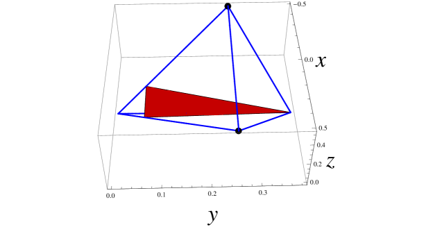
Figure 1: (Color online) Each point in tetrahedron is correspondent to the GHZ-symmetric state. Two black dots represent the $4$-qubit GHZ state $\lvert\mbox{GHZ}_{4}\rangle_{\pm}$. The surface of triangle in the tetrahedron is the place where the RGHZ-symmetric states reside. (b) Each point in triangle is correspondent to the RGHZ-symmetric state. This triangle is equivalent to the triangle in Fig. 1(a). Thus, RGHZ symmetric states have very small portion and are of zero measure in the whole set of the GHZ-symmetric states.

In order for $\rho_{4}^{\mbox{\scriptsize{GHZ}}}$ to be a physical state the parameters should be restricted to

$$0\leq\tilde{\alpha}_{2}\leq\frac{1}{8}\hskip 28.45274pt0\leq\tilde{\alpha}_{3}\leq\frac{1}{6}\hskip 28.45274pt0\leq\tilde{\alpha}_{1}\leq\frac{1}{2}$$ (9)

and

$$\tilde{\alpha}_{1}\geq\pm\tilde{x}.$$ (10)

This physical conditions imply that any GHZ-symmetric physical state is represented as a point inside a tetrahedron shown in Fig. 1(a). In this figure two black dots represent $\lvert\mbox{GHZ}_{4}\rangle_{\pm}$, respectively. It is worthwhile noting that the sign of $x$ does not change the character of entanglement because $\rho_{4}^{\mbox{\scriptsize{GHZ}}}(-\tilde{x},\tilde{y},\tilde{z})=u\rho_{4}^{\mbox{\scriptsize{GHZ}}}(\tilde{x},\tilde{y},\tilde{z})u^{\dagger}$, where $u=i\sigma_{x}\otimes\sigma_{y}\otimes\sigma_{y}\otimes\sigma_{y}$.

II.2 RGHZ-symmetric states

It is straightforward to show that the general form of RGHZ-symmetric states is

$$\hskip 71.13188pt\rho_{4}^{\mbox{\scriptsize{RGHZ}}}=x\left[\lvert 0000\rangle\langle 1111\lvert+\lvert 1111\rangle\langle 0000\lvert\right]$$ (11)

$$+\mbox{diag}\left(\alpha_{1},\alpha_{2},\alpha_{2},\alpha_{1},\alpha_{2},\alpha_{1},\alpha_{1},\alpha_{2},\alpha_{2},\alpha_{1},\alpha_{1},\alpha_{2},\alpha_{1},\alpha_{2},\alpha_{2},\alpha_{1}\right)$$

with $\alpha_{1}=\frac{1}{16}+\frac{y}{2\sqrt{2}}$ and $\alpha_{2}=\frac{1}{16}-\frac{y}{2\sqrt{2}}$. The parameters $x$ and $y$ are chosen such that the Euclidean metric in the $(x,y)$ plane coincides with the Hilbert-Schmidt metric $d^{2}(A,B)=\frac{1}{2}\mbox{tr}(A-B)^{\dagger}(A-B)$ again. The parameters can be represented as

$$x=\frac{1}{2}\left[{}_{+}\langle\mbox{GHZ}_{4}\lvert\rho_{4}^{\mbox{\scriptsize{RGHZ}}}\lvert\mbox{GHZ}_{4}\rangle_{+}-_{-}\langle\mbox{GHZ}_{4}\lvert\rho_{4}^{\mbox{\scriptsize{RGHZ}}}\lvert\mbox{GHZ}_{4}\rangle_{-}\right]$$

$$y=\sqrt{2}\left[{}_{+}\langle\mbox{GHZ}_{4}\lvert\rho_{4}^{\mbox{\scriptsize{RGHZ}}}\lvert\mbox{GHZ}_{4}\rangle_{+}+_{-}\langle\mbox{GHZ}_{4}\lvert\rho_{4}^{\mbox{\scriptsize{RGHZ}}}\lvert\mbox{GHZ}_{4}\rangle_{-}-\frac{1}{8}\right].$$

It is also worthwhile noting that the sign of $x$ does not change the entanglement because $\rho_{4}^{\mbox{\scriptsize RGHZ}}(-x,y)=u\rho_{4}^{\mbox{\scriptsize RGHZ}}(x,y)u^{\dagger}$. This is evident from the fact that the RGHZ-symmetric state is also GHZ-symmetric.

Since $\rho_{4}^{\mbox{\scriptsize RGHZ}}$ is a quantum state, it should be a positive operator, which restricts the parameters as

$$y\geq\pm 2\sqrt{2}x-\frac{\sqrt{2}}{8}\hskip 56.9055pt|x|\leq\frac{1}{8}.$$ (13)

Thus any RGHZ-symmetric physical state is represented as a point in a triangle depicted in Fig. 1(b).

It is easy to show that $\rho_{4}^{\mbox{\scriptsize{GHZ}}}$ is RGHZ-symmetric if and only if $\tilde{x}=x$, $\tilde{\alpha}_{2}=\alpha_{2}$, and $\tilde{\alpha_{1}}=\tilde{\alpha}_{3}=\alpha_{1}$ or equivalently

$$\tilde{y}={\cal N}_{1}\left[\frac{\sqrt{10}+4}{16}-\frac{\sqrt{10}+2}{2\sqrt{2}}y\right]\hskip 28.45274pt\tilde{z}={\cal N}_{2}\left[\frac{\sqrt{10}+2}{16}+\frac{\sqrt{10}+4}{2\sqrt{2}}y\right].$$ (14)

Using this relation it is possible to know where the RGHZ-symmetric states reside in the tetrahedron in Fig. 1(a). In this figure the red triangle is equivalent one of Fig. 1(b). Thus, the states on this triangle are RGHZ-symmetric. From Fig. 1(a) one can realize that the RGHZ-symmetric states have very small portion and are of zero measure in the entire set of GHZ-symmetric states.

III SLOCC Classification of RGHZ-symmetric States

The SLOCC classification of the $4$-qubit pure-state system was first discussed in fourP-1 by making use of the Jordan block structure of some complex symmetric matrix. Subsequently, same issue was explored in several more papers using different approachesfourP-2 . Unlike, however, two- and three-qubit cases, the results of Ref.fourP-1 ; fourP-2 seem to be contradictory to each other. This means that still our understanding on the $4$-qubit entanglement is incomplete.

In this paper we adopt the results of fourP-1 , where there are following nine inequivalent SLOCC classes;

$$G_{abcd} = \frac{a+d}{2}(|0000\rangle+|1111\rangle)+\frac{a-d}{2}(|0011\rangle+|1100\rangle)$$

$$\hskip 2.84544pt+\frac{b+c}{2}(|0101\rangle+|1010\rangle)+\frac{b-c}{2}(|0110\rangle+|1001\rangle)$$

$$L_{abc_{2}} = \frac{a+b}{2}(|0000\rangle+|1111\rangle)+\frac{a-b}{2}(|0011\rangle+|1100\rangle)$$

$$\hskip 14.22636pt+c(|0101\rangle+|1010\rangle)+|0110\rangle$$

$$L_{a_{2}b_{2}} = a(|0000\rangle+|1111\rangle)+b(|0101\rangle+|1010\rangle)+|0110\rangle+|0011\rangle$$

$$L_{ab_{3}} = a(|0000\rangle+|1111\rangle)+\frac{a+b}{2}(|0101\rangle+|1010\rangle)$$

$$\hskip 2.84544pt+\frac{a-b}{2}(|0110\rangle+|1001\rangle)+\frac{i}{\sqrt{2}}(|0001\rangle+|0010\rangle+|0111\rangle+|1011\rangle)$$

$$L_{a_{4}} = a(|0000\rangle+|0101\rangle+|1010\rangle+|1111\rangle)+(i|0001\rangle+|0110\rangle-i|1011\rangle)$$

$$L_{a_{2}0_{3\oplus\bar{1}}} = a(|0000\rangle+|1111\rangle)+(|0011\rangle+|0101\rangle+|0110\rangle)$$

$$L_{0_{5\oplus\bar{3}}} = |0000\rangle+|0101\rangle+|1000\rangle+|1110\rangle$$

$$L_{0_{7\oplus\bar{1}}} = |0000\rangle+|1011\rangle+|1101\rangle+|1110\rangle$$

$$L_{0_{3\oplus\bar{1}}0_{3\oplus\bar{1}}} = |0000\rangle+|0111\rangle,$$

where $a$, $b$, $c$, and $d$ are complex parameters with nonnegative real part. In Eq. (III) $G_{abcd}$ is special in a sense that its all local states are completely mixed. In other words, $G_{abcd}$ is a set of normal statesverst03 .

III.1 $L_{abc_{2}}$

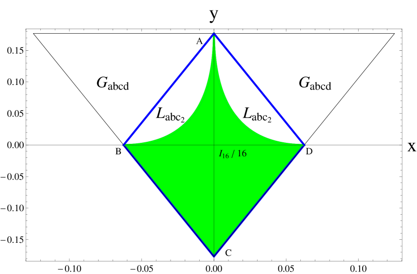
Figure 2: (Color online) The SLOCC classification of RGHZ-symmetric states $\rho_{4}^{\mbox{\scriptsize{RGHZ}}}$. In the polygon ABCD states of $L_{abc_{2}}$ reside. Theorem 2 implies that there is no one-qubit tensor product three-qubit entangled states in the GHZL-symmetric states. This fact implies that the RGHZ symmetry exclude $L_{a_{2}0_{3\oplus\bar{1}}}$, $L_{0_{3\oplus\bar{1}}0_{3\oplus\bar{1}}}$, and $L_{a_{2}b_{2}}$. Theorem 3 implies that there are states of $G_{abcd}$ outside the polygon ABCD.

In this subsection we examine a question where the states of $L_{abc_{2}}$ reside in the triangle in Fig. 1(b). Before proceeding further, it is important to note that there is a correspondence between four-qubit pure states and RGHZ-symmetric states. Let $\lvert\psi\rangle$ be a four-qubit pure state. Then, the corresponding RGHZ-symmetric state $\rho_{4}^{\mbox{\scriptsize{RGHZ}}}(\psi)$ can be written as

$$\rho_{4}^{\mbox{\scriptsize{RGHZ}}}(\psi)=\int U\lvert\psi\rangle\langle\psi\lvert U^{\dagger},$$ (16)

where the integral is understood to cover the entire RGHZ symmetry group, i.e., unitaries $U(\phi_{1},\phi_{2},\phi_{3})$ in Eq. (2) and averaging over the discrete symmetries. For example, if $\lvert\psi\rangle=\sum_{i,j,k,l=0}^{1}\psi_{ijkl}\lvert ijkl\rangle$, $\rho_{4}^{\mbox{\scriptsize{RGHZ}}}(\psi)$ becomes Eq. (11) with

$$x=\frac{1}{4}\mbox{Re}\bigg{[}\psi_{0000}\psi_{1111}^{*}+\psi_{0011}\psi_{1100}^{*}+\psi_{0101}\psi_{1010}^{*}+\psi_{0110}\psi_{1001}^{*}\bigg{]}$$ (17)

$$\alpha_{1}\equiv\frac{1}{16}+\frac{y}{2\sqrt{2}}=\frac{1}{8}\bigg{[}|\psi_{0000}|^{2}+|\psi_{1111}|^{2}+|\psi_{0011}|^{2}+|\psi_{0101}|^{2}$$

$$\hskip 113.81102pt+|\psi_{0110}|^{2}+|\psi_{1001}|^{2}+|\psi_{1010}|^{2}+|\psi_{1100}|^{2}\bigg{]}.$$

Now, we are ready to discuss the main issue of this subsection.

Theorem 1. The RGHZ-symmetric states of $L_{abc_{2}}$-class reside in the polygon ABCD in Fig. 2.

Proof. First we note that when $a=b=c=0$, $L_{abc_{2}}$ reduces to the fully separable state $\lvert 0110\rangle$. Since LU is a particular case of SLOCC, this fact implies that all fully separable states are in the $L_{abc_{2}}$. Let $\lvert\psi^{sep}\rangle=(u_{1}\otimes u_{2}\otimes u_{3}\otimes u_{4})\lvert 0000\rangle$, where

$$u_{j}=\left(\begin{array}[]{cc}A_{j}&-C_{j}^{*}\\ C_{j}&A_{j}^{*}\end{array}\right)\hskip 28.45274pt\mbox{with}\hskip 5.69046pt|A_{j}|^{2}+|C_{j}|^{2}=1.$$ (20)

Then, it is easy to derive the parameters $x$ and $y$ of $\rho_{4}^{\mbox{\scriptsize{RGHZ}}}(\psi^{sep})$ easily using Eq. (17). Our method for proof is as follows. Applying the Lagrange multiplier method we maximize $x$ with given $y$. Then, it is possible to derive a boundary $x_{\max}=x_{\max}(y)$ in the $(x,y)$ plane. If a region inside the boundary is convex, this is the region where the $L_{abc_{2}}$-class states reside. If it is not convex, we have to choose the convex hull of it for the residential region.

From a symmetry it is evident that the maximum of $x$ occurs when $A_{1}=A_{2}=A_{3}=A_{4}\equiv A$. Then the constraint of $y$ yields $A^{2}=\frac{1}{2}\left(1\pm 2^{5/8}y^{1/4}\right)$, which gives

$$x_{max}=\frac{1}{16}\left(1-2^{\frac{5}{4}}y^{\frac{1}{2}}\right)^{2}.$$ (21)

Since the sign of $x_{max}$ does not change the entanglement class, the region represented by green color in Fig. 2 is derived. Since it is not convex, we have to choose a convex hull, which is a polygon ABCD in Fig. 2. This completes the proof.

Although we start with fully separable state, this does not guarantee that all states in the polygon ABCD are fully separable because $L_{abc_{2}}$ has $4$-way entangled states as well as fully separable states. The only fact we can assert is that all $L_{abc_{2}}$-class RGHZ-symmetric states reside in the polygon ABCD.

III.2 $L_{a_{2}0_{3\oplus\bar{1}}},L_{0_{3\oplus\bar{1}}0_{3\oplus\bar{1}}},\cdots$

In this subsection we will show that the RGHZ symmetry excludes all SLOCC classes except $G_{abcd}$.

Theorem 2. There is no one-qubit product GHZ state in the RGHZ-symmetric states.

Proof. Let $\lvert\psi^{GHZ}\rangle=(G_{1}\otimes G_{2}\otimes G_{3}\otimes G_{4})\lvert 0\rangle\otimes(\lvert 000\rangle+\lvert 111\rangle)$, where

$$G_{j}=\left(\begin{array}[]{cc}A_{j}&B_{j}\\ C_{j}&D_{j}\end{array}\right).$$ (24)

Then, it is easy to compute $x$ and $y$ of $\rho_{4}^{\mbox{\scriptsize{RGHZ}}}(\psi^{GHZ})$ using Eq. (17). Now, we want to maximize $x$ with given $y$ and $\langle\psi^{GHZ}\lvert\psi^{GHZ}\rangle=1$. From symmetry of the Lagrange multiplier equations it is evident that the maximum of $x$ occurs when $A_{2}=A_{3}=A_{4}=B_{2}=B_{3}=B_{4}\equiv a$ and $C_{2}=C_{3}=C_{4}=D_{2}=D_{3}=D_{4}\equiv c$. Then, we define $x^{\Lambda}=x+\Lambda_{0}\Theta_{0}+\Lambda_{1}\Theta_{1}$, where $\Lambda_{0}$ and $\Lambda_{1}$ are Lagrange multiplier constants, and

$$x=4A_{1}C_{1}a^{3}c^{3}$$ (25)

$$\Theta_{0}=4(A_{1}^{2}+C_{1}^{2})(a^{2}+c^{2})^{2}-1$$

$$\Theta_{1}=4\left[A_{1}^{2}a^{2}(a^{4}+3c^{4})+C_{1}^{2}c^{2}(3a^{4}+c^{4})-2\alpha_{1}\right].$$

Now, we want to maximize $x$ under the constraints $\Theta_{0}=\Theta_{1}=0$.

First, we solve the two constraints, whose solutions are

$$A_{1}^{2}=\frac{8\alpha_{1}(u_{1}+u_{2})-u_{2}}{u_{1}^{2}-u_{2}^{2}}\hskip 56.9055ptC_{1}^{2}=\frac{u_{1}-8\alpha_{1}(u_{1}+u_{2})}{u_{1}^{2}-u_{2}^{2}},$$ (26)

where $u_{1}=4a^{2}(a^{4}+3c^{4})$ and $u_{2}=4c^{2}(3a^{4}+c^{4})$. From $\frac{\partial x^{\Lambda}}{\partial A_{1}}=\frac{\partial x^{\Lambda}}{\partial C_{1}}=0$ one can express the Lagrange multiplier constants as

$$\Lambda_{0}=-\frac{A_{1}^{2}u_{1}-C_{1}^{2}u_{2}}{A_{1}C_{1}}\frac{2a^{3}c^{3}}{u_{1}^{2}-u_{2}^{2}}\hskip 56.9055pt\Lambda_{1}=\frac{A_{1}^{2}-C_{1}^{2}}{A_{1}C_{1}}\frac{2a^{3}c^{3}}{u_{1}-u_{2}}.$$ (27)

Combining Eqs. (26), (27), and $\frac{\partial x^{\Lambda}}{\partial a}=\frac{\partial x^{\Lambda}}{\partial c}=0$, we obtain

$$8\alpha_{1}(z^{2}+1)^{4}=z^{8}+6z^{4}+1,$$ (28)

where $z=\frac{a}{c}$. Then, the maximum of $x$ with given $y$ becomes

$$x_{max}=\frac{z^{3}\sqrt{8\alpha_{1}(1-8\alpha_{1})(1+z^{2})^{6}-z^{2}(3+z^{4})(1+3z^{4})}}{(z^{4}-1)^{3}}.$$ (29)

Using Eq. (28) and performing long and tedious calculation, one can show that the right-hand side of Eq. (29) reduces to $\frac{1}{16}\left(1-\sqrt{16\alpha_{1}-1}\right)^{2}$, which results in the identical equation with Eq. (21). This implies that there is no one-qubit product three-qubit GHZ state in the RGHZ-symmetric states. This completes the proof.

From this theorem one can conclude that there is no $L_{0_{3\oplus\bar{1}}0_{3\oplus\bar{1}}}$ in the RGHZ-symmetric states, because this class involves one-qubit product GHZ-state. Since it is well-known that the three-qubit states consist of fully separable (S), bi-separable (B), W, and GHZ states, and they satisfy a linear hierarchy S $\subset$ B $\subset$ W $\subset$ GHZ, theorem 2 also implies that there is no one-qubit product W state in the RGHZ-symmetric states. Thus, RGHZ symmetry excludes $L_{a_{2}0_{3\oplus\bar{1}}}$ too because this class contains one-qubit product W state when $a=0$. This theorem also implies that there is no one-qubit product one-qubit product B state, which excludes $L_{a_{2}b_{2}}$. Similarly, one can exclude all classes except $G_{abcd}$-class.

III.3 $G_{abcd}$

Now, we want to discuss the entanglement classes of remaining RGHZ-symmetric states. In order to conjecture the classes quickly, let us consider the following double bi-separable state

$$\lvert\psi^{BB}\rangle=\frac{1}{\sqrt{2}}\left(\lvert 00\rangle+\lvert 11\rangle\right)\otimes\frac{1}{\sqrt{2}}\left(\lvert 00\rangle+\lvert 11\rangle\right).$$ (30)

Such a state belongs to $G_{abcd}$ with $(a=1,b=c=d=0)$ or $a=b=c=d$. Then, Eq. (17) shows that the parameters of $\rho_{4}^{\mbox{\scriptsize{GHZL}}}(\psi^{BB})$ are $x=1/8$ and $y=\sqrt{2}/8$, which correspond to the right-upper corner of the triangle in Fig. 2. Since mixing can result only in the same or a lower entanglement class, the entanglement class of this corner state should be $G_{abcd}$ or its sub-classes. However, the sub-class of this state should be a class, where fully separable states belong, and those states are confined in $ABCD$. Therefore, the corner should be $G_{abcd}$. This fact strongly suggests that all remaining states in Fig. 2 are $G_{abcd}$. The following theorem shows that our conjecture is correct.

Theorem 3. All remaining RGHZ-symmetric states in Fig. 2 are $G_{abcd}$-class.

Proof. Let $\lvert\psi^{BB}\rangle=(G_{1}\otimes G_{2}\otimes G_{3}\otimes G_{4})(\lvert 00\rangle+\lvert 11\rangle)\otimes(\lvert 00\rangle+\lvert 11\rangle)$, where $G_{j}$ is given in Eq. (24). Then, it is easy to compute the parameters $x$ and $y$ of $\rho_{4}^{\mbox{\scriptsize{GHZL}}}(\psi^{BB})$ using Eq. (17). Similar to the previous theorems we want to maximize $x$ with given $y$. From a symmetry of Lagrange multiplier equations it is evident that the maximum of $x$ occurs when

$$A_{1}=A_{2}\equiv a_{1}\hskip 42.67912ptA_{3}=A_{4}\equiv a_{3}$$ (31)

$$B_{1}=B_{2}\equiv b_{1}\hskip 42.67912ptB_{3}=B_{4}\equiv b_{3}$$

$$C_{1}=C_{2}\equiv c_{1}\hskip 42.67912ptC_{3}=C_{4}\equiv c_{3}$$

$$D_{1}=D_{2}\equiv d_{1}\hskip 42.67912ptD_{3}=D_{4}\equiv d_{3}.$$

For later convenience we define $\mu_{1}=a_{1}^{2}+b_{1}^{2}$, $\mu_{2}=a_{3}^{2}+b_{3}^{2}$, $\mu_{3}=c_{1}^{2}+d_{1}^{2}$, $\mu_{4}=c_{3}^{2}+d_{3}^{2}$, $\nu_{1}=a_{1}c_{1}+b_{1}d_{1}$, and $\nu_{2}=a_{3}c_{3}+b_{3}d_{3}$.

In order to apply the Lagrange multiplier method we define $x^{\Lambda}=x+\Lambda_{0}\Theta_{0}+\Lambda_{1}\Theta_{1}$, where

$$x=\frac{1}{2}\left(\mu_{1}\mu_{2}\mu_{3}\mu_{4}+\nu_{1}^{2}\nu_{2}^{2}\right)$$ (32)

$$\Theta_{0}=(\mu_{1}^{2}+2\nu_{1}^{2}+\mu_{3}^{2})(\mu_{2}^{2}+2\nu_{2}^{2}+\mu_{4}^{2})-1$$

$$\Theta_{1}=(\mu_{1}^{2}+\mu_{3}^{2})(\mu_{2}^{2}+\mu_{4}^{2})+4\nu_{1}^{2}\nu_{2}^{2}-8\alpha_{1}.$$

The constraints $\Theta_{0}=0$ and $\Theta_{1}=0$ come from $\langle\psi^{BB}\lvert\psi^{BB}\rangle=1$ and Eq. (17), respectively.

Now, we have eight equations $\frac{\partial x^{\Lambda}}{\partial\mu_{i}}=0\hskip 5.69046pt(i=1,2,3,4)$, $\frac{\partial x^{\Lambda}}{\partial\nu_{i}}=0\hskip 5.69046pt(i=1,2)$, and $\Theta_{0}=\Theta_{1}=0$. Analyzing those equations, one can show that the maximum of $x$ occurs when $\mu_{1}=\mu_{3}$ and $\mu_{2}=\mu_{4}$. Then, the constraint $\Theta_{1}=0$ implies

$$x_{max}=\frac{1}{16}+\frac{y}{2\sqrt{2}},$$ (33)

which corresponds to the right side of the triangle in Fig. 2. This fact implies that the whole RGHZ-symmetric states are $G_{abcd}$ or its sub-class. Since $L_{abc_{2}}$ are confined in the polygon ABCD and the remaining classes except $G_{abcd}$ are already excluded, the states outside the polygon ABCD should be $G_{abcd}$-class, which completes the proof.

Although we start with a double bi-separable state, this fact does not implies that all states outside the polygon are double bi-separable because $G_{abcd}$ contains $4$-way entangled states as well as double bi-separable states. The only fact we can say is that all states outside the polygon ABCD are $G_{abcd}$-class.

IV conclusion

In this paper the GHZ and RGHZ symmetries in four-qubit system are examined. It is shown that the whole RGHZ-symmetric states involve only two SLOCC classes, $L_{abc_{2}}$ and $G_{abcd}$. Following Ref. elts12-2 we can use our result to construct the optimal witness $\mathcal{W}_{\mathrm{G_{abcd}\setminus L_{abc_{2}}}}$, which can detect the $G_{abcd}$-class optimally from a set of $L_{abc_{2}}$ plus $G_{abcd}$ states.

As remarked earlier if we choose GHZ symmetry, the symmetric states are represented by three real parameters as Eq. (4) shows. Probably, these symmetric states involve more kinds of the four-qubit SLOCC classes. The SLOCC classification of Eq. (4) will be explored in the future.

Another interesting extension of present paper is to generalize our analysis to any $2n$-qubit system. Then, our modification of symmetry should be changed into ‘any one-pair, two-pair, $\cdots$, and $n$-pair flips’. This would drastically reduce the number of free parameters in the set of symmetric states. This strongly restricted symmetry may shed light on the SLOCC classification of the multipartite states.

Acknowledgement: This work was supported by the Kyungnam University Foundation Grant, 2013.

References

• (1) R. Horodecki, P. Horodecki, M. Horodecki, and K. Horodecki, Quantum Entanglement, Rev. Mod. Phys. 81 (2009) 865 [quant-ph/0702225] and references therein.
• (2) C. H. Bennett, G. Brassard, C. CrΒ΄epeau, R. Jozsa, A. Peres and W. K. Wootters, Teleporting an Unknown Quantum State via Dual Classical and Einstein-Podolsky-Rosen Channles, Phys.Rev. Lett. 70 (1993) 1895.
• (3) C. H. Bennett and S. J. Wiesner, Communication via one- and two-particle operators on Einstein-Podolsky-Rosen states, Phys. Rev. Lett. 69 (1992) 2881.
• (4) V. Scarani, S. Lblisdir, N. Gisin and A. Acin, Quantum cloning, Rev. Mod. Phys. 77 (2005) 1225 [quant-ph/0511088] and references therein.
• (5) A. K. Ekert, Quantum Cryptography Based on Bell’s Theorem, Phys. Rev. Lett. 67 (1991) 661.
• (6) M. A. Nielsen and I. L. Chuang, Quantum Computation and Quantum Information (Cambridge University Press, Cambridge, England, 2000).
• (7) G. Vidal, Efficient classical simulation of slightly entangled quantum computations, Phys. Rev. Lett. 91 (2003) 147902 [quant-ph/0301063].
• (8) C. H. Bennett, S. Popescu, D. Rohrlich, J. A. Smolin, and A. V. Thapliyal, Exact and asymptotic measures of multipartite pure-state entanglement, Phys. Rev. A 63 (2000) 012307 [quant-ph/9908073].
• (9) G. Vidal, Entanglement monotones, J. Mod. Opt. 47 (2000) 355 [quant-ph/9807077].
• (10) W. DΓΌr, G. Vidal and J. I. Cirac, Three qubits can be entangled in two inequivalent ways, Phys.Rev. A 62 (2000) 062314.
• (11) V. Coffman, J. Kundu and W. K. Wootters, Distributed entanglement, Phys. Rev. A 61 (2000) 052306 [quant-ph/9907047].
• (12) W. K. Wootters, Entanglement of Formation of an Arbitrary State of Two Qubits, Phys. Rev. Lett. 80 (1998) 2245 [quant-ph/9709029].
• (13) A. AcΓ­n, D. Bruß, M. Lewenstein, and A. Sanpera, Classification of Mixed Three-Qubit States, Phys. Rev. Lett. 87 (2001) 040401.
• (14) R. Lohmayer, A. Osterloh, J. Siewert and A. Uhlmann, Entangled Three-Qubit States without Concurrence and Three-Tangle, Phys. Rev. Lett. 97 (2006) 260502 [quant-ph/0606071]; C. Eltschka, A. Osterloh, J. Siewert and A. Uhlmann, Three-tangle for mixtures of generalized GHZ and generalized W states, New J. Phys. 10 (2008) 043014 [arXiv:0711.4477 (quant-ph)]; E. Jung, M. R. Hwang, D. K. Park and J. W. Son, Three-tangle for Rank-$3$ Mixed States: Mixture of Greenberger-Horne-Zeilinger, W and flipped W states, Phys. Rev. A 79 (2009) 024306 [arXiv:0810.5403 (quant-ph)]; E. Jung, D. K. Park, and J. W. Son, Three-tangle does not properly quantify tripartite entanglement for Greenberger-Horne-Zeilinger-type state, Phys. Rev. A 80 (2009) 010301(R) [arXiv:0901.2620 (quant-ph)]; E. Jung, M. R. Hwang, D. K. Park, and S. Tamaryan, Three-Party Entanglement in Tripartite Teleportation Scheme through Noisy Channels, Quant. Inf. Comput. 10 (2010) 0377 [arXiv:0904.2807 (quant-ph)].
• (15) C. Eltschka and J. Siewert, Entanglement of Three-Qubit Greenberger-Horne-Zeilinger-Symmetric States, Phys. Rev. Lett. 108 (2012) 020502 [arXiv:1304.6095 (quant-ph)].
• (16) J. Siewert and C. Eltschka, Quantifying Tripartite Entanglement of Three-Qubit Generalized Werner States, Phys. Rev. Lett. 108 (2012) 230502.
• (17) C. Eltschka and J. Siewert, Optimal witnesses for three-qubit entanglement from Greenberger-Horne-Zeilinger symmetry, Quant. Inf. Comput. 13 (2013) 0210 (2013) [arXiv:1204.5451 (quant-ph)].
• (18) C. Eltschka and J. Siewert, Practical method to obtain a lower bound to the three-tangle, Phys. Rev. A 89 (2014) 022312 [arXiv:1310.8311 (quant-ph)].
• (19) Eylee Jung and DaeKil Park, Entanglement Classification of relaxed Greenberger-Horne-Zeilinger-Symmetric States, Quant. Inf. Comput. 14 (2014) 0937 [arXiv:1303.3712 (quant-ph)].
• (20) A. Osterloh and J. Siewert, Entanglement monotones and maximally entangled states in multipartite qubit systems, Quant. Inf. Comput. 4 (2006) 0531 [quant-ph/0506073].
• (21) F. Verstraete, J. Dehaene, B. De Moor, and H. Verschelde, Four qubits can be entangled in nine different ways, Phys. Rev. A 65 (2002) 052112 [quant-ph/0109033].
• (22) L. Lamata, J. LeΓ³n, D. Salgado, and E. Solano, Inductive entanglement of four qubits under stochastic local operations and classical communication, Phys. Rev. A 75 (2007) 022318 [quant-ph/0603243]; Y. Cao and A. M. Wang, Discussion of the entanglement classification of a 4-qubit pure state, Eur. Phys. J. D 44 (2007) 159; O. Chterental and D. Z. DjokovΓ­c, in Linear Algebra Research Advances, edited by G. D. Ling (Nova Science Publishers, Inc., Hauppauge, NY, 2007), Chap. 4, pp. 133-167; D. Li, X. Li, H. Huang, and X. Li, SLOCC Classification for Nine Families of Four-Qubits, Quant. Inf. Comput. 9 (2009) 0778 [arXiv:0712.1876 (quant-ph)]; S. J. Akhtarshenas and M. G. Ghahi, Entangled graphs: A classification of four-qubit entanglement, arXiv:1003.2762 (quant-ph); L. Borsten, D. Dahanayake, M. J. Duff, A. Marrani, and W. Rubens, Four-Qubit Entanglement Classification from String Theory, Phys. Rev. Lett. 105 (2010) 100507 [arXiv:1005.4915 (hep-th)].
• (23) F. Verstraete, J. Dehaene, and D. De Moor, Normal forms and entanglement measures for multipartite quantum states, Phys. Rev. A 68 (2003) 012103 [quant-ph/0105090].