Stochastic extension of the Lanczos method for nuclear shell-model calculations with variational Monte Carlo method

Abstract

We propose a new variational Monte Carlo (VMC) approach based on the Krylov subspace for large-scale shell-model calculations. A random walker in the VMC is formulated with the $M$-scheme representation, and samples a small number of configurations from a whole Hilbert space stochastically. This VMC framework is demonstrated in the shell-model calculations of ⁴⁸Cr and ⁶⁰Zn, and we discuss its relation to a small number of Lanczos iterations. By utilizing the wave function obtained by the conventional particle-hole-excitation truncation as an initial state, this VMC approach provides us with a sequence of systematically improved results.

I Introduction

Large-scale shell model calculations in the nuclear structure study are performed by solving an eigenvalue problem of a large-dimension sparse matrix. The Krylov-subspace method is one of the best tools, and practically the only solution to solve the problem efficiently krylov . The Krylov subspace is spanned by a starting vector $v$ and the product of the first $p$ powers of the Hamiltonian matrix $H$, namely $\{v,Hv,H^{2}v,\cdot\cdot\cdot,H^{p}v\}$. An eigenvalue of the Hamiltonian matrix in Krylov subspace is called the Ritz value, and it is known to converge in a small number of iterations to the largest (or smallest) eigenvalue, since $H^{p}v$ with large $p$ is dominated by the eigenvectors which have the large absolute eigenvalue. In the Krylov-subspace method, the converged Ritz value becomes a good approximation to the exact eigenvalue. Since the construction of the Krylov subspace requires only the matrix-vector product, the Krylov-subspace method has been extensively used and developed to solve an eigenvalue problem of a huge sparse matrix.

In the case of nuclear shell-model calculations, the Hamiltonian matrix in $M$-scheme basis is very sparse since the Hamiltonian consists of one-body and two-body interactions. The needed dimension of the Hamiltonian matrix is often quite huge, therefore, the Krylov-subspace iteration algorithm is quite efficient. The Lanczos algorithm, one of the most famous Krylov subspace algorithms, was introduced in 70’s, lanczos ; lanczos-sebe ; M-lanczos and has been widely used in shell-model calculations. Nowadays, it is implemented to take advantage of massively parallel computations mfdn .

Nevertheless, the application is still hampered by the exponential growth of the dimension of the Hilbert space. The size of a state vector surpasses the capacity of memory and the truncation of the model space is required. The most naive truncation is to assume a Fermi level for single-particle occupation and to restrict the number of particle-hole excitation across the Fermi level up to $t$ particles. It is called the $t$-particle $t$-hole truncation and frequently used in practical calculations. As $t$ increases, the eigenstate in the truncated subspace approaches the true eigenstate rather gradually. However, the significance of the large $t$ component remains and is difficult to estimate (e.g. horoi_ni56 ) due to the limitation of computational resources.

On the other hand, much effort has been paid to circumvent this problem by introducing the Markov Chain Monte Carlo (MCMC) in the context of quantum Monte Carlo smmc ; rombouts . However, the notorious “sign problem” prohibits to use realistic shell-model interaction practically.

In the present work, to estimate the omitted contribution of $t$-particle $t$-hole truncation for the exact shell-model energy in full Hilbert space we introduce the variational Monte Carlo (VMC) approach into the shell-model calculations, and show that this VMC can overcome the limitation of the truncation scheme without treating the basis vectors of the full Hilbert space explicitly.

II Formulation

We describe the form of a trial wave function of this VMC approach. At the beginning, we calculate the lowest eigenstate in the $t$-particle $t$-hole truncated subspace, $|\psi^{t}\rangle$. Then, we introduced the VMC approach combined with the Krylov-subspace method with $|\psi^{t}\rangle$ being a starting vector to improve the approximation systematically.

The Ritz vector, or the approximated eigenvector on the Krylov subspace is taken as a trial wave function such as

$$|\Psi({\bf c})\rangle=\left(\sum_{q=0}^{p}c_{q}H^{q}\right)|\psi^{t}\rangle$$ (1)

where $H$ is the Hamiltonian and ${\bf c}=\{c_{0},c_{1},c_{2},...,c_{p}\}$ is a set of variational parameters, which are determined by minimizing the energy expectation value. The $|\psi^{t}\rangle$ is represented by a linear combination of the $M$-scheme basis states, that is, $|m\rangle=c^{\dagger}_{m_{1}}c^{\dagger}_{m_{2}}...c^{\dagger}_{m_{A}}|-\rangle$ where $c^{\dagger}_{m}$ is a creation operator of the single-particle state, $m$, and $|-\rangle$ stands for an inert core.

The energy expectation value of the trial wave function is written by inserting the complete set of the $M$-scheme subspace, $1=\sum_{m\in\{M^{\pi}\}}|m\rangle\langle m|$, where $|m\rangle$ has a fixed $z$-component of angular momentum $M$ and parity $\pi$, such as

$$E({\bf c}) = \frac{\langle\Psi|H|\Psi\rangle}{\langle\Psi|\Psi\rangle}=\frac{\sum_{m\in\{M^{\pi}\}}|\langle m|\Psi\rangle|^{2}\frac{\langle m|H|\Psi\rangle}{\langle m|\Psi\rangle}}{\sum_{m\in\{M^{\pi}\}}|\langle m|\Psi\rangle|^{2}}.$$ (2)

Since the number of $M$-scheme states rapidly increase as a function of the particle number and the size of the single-particle space, the practical summation of $|m\rangle$ in Eq.(2) often becomes difficult to perform. Therefore, we apply the Monte Carlo technique to this summation and calculate the energy expectation value $E({\bf c})$ stochastically. The Monte Carlo random walker of $m$ state is formulated in the $M$-scheme basis obeying the probability proportional to $|\langle m|\Psi({\bf c})\rangle|^{2}$. The complete set of $|m\rangle$ is represented by the $N$ samples of the random walkers as

$$E({\bf c}) \sim \frac{1}{N}\sum_{m\in{\rm M.C.}}E_{\rm local}(m,{\bf c})$$ (3)

with the local energy

$$E_{\rm local}(m,{\bf c})=\frac{\langle m|H|\Psi({\bf c})\rangle}{\langle m|\Psi({\bf c})\rangle}$$ (4)

and the sampling density

$$\rho_{\bf c}(m)=\frac{|\langle m|\Psi({\bf c})\rangle|^{2}}{|\sum_{m^{\prime}}\langle m^{\prime}|\Psi({\bf c})\rangle|^{2}}.$$ (5)

The $\sum_{m\in{\rm M.C.}}$ denotes the summation of $N$ samples, $m$, which are generated by the $M$-scheme random walker with the probability density $\rho_{\bf c}(m)$.

In order to compute the $E({\bf c})$ in Eq.(3) stochastically, we briefly describe the MCMC process to generate a random walker in $M$-scheme basis states. It was first introduced in Ref. vmcsm .

The transition of the random walker is controlled by the Metropolis algorithm. The candidate of the transition is created by two-particle two-hole operator like $|m^{\prime}\rangle=c^{\dagger}_{i}c^{\dagger}_{j}c_{k}c_{l}|m\rangle$ with $c^{\dagger}_{i}$ being the creation operator of a single-particle state $i$. The indices, $i,j,k,$ and $l$, are restricted so that $|m\rangle$ and $|m^{\prime}\rangle$ having the same $z$-component of angular momentum and parity. Whether or not a random walker $|m\rangle$ moves to $|m^{\prime}\rangle$ depends on the ratio $p_{\bf c}(m^{\prime})=\rho(m^{\prime})/\rho(m)$ as

$$p_{\bf c}(m^{\prime})=\left|\frac{\langle m^{\prime}|\Psi({\bf c})\rangle}{\langle m|\Psi({\bf c})\rangle}\right|^{2}.$$ (6)

If $p_{\bf c}(m^{\prime})\geq 1$, the walker $|m\rangle$ always moves to $|m^{\prime}\rangle$. If $p_{\bf c}(m^{\prime})<1$, according to the $p_{\bf c}(m^{\prime})$, we determine whether or not the walker $|m\rangle$ moves to $|m^{\prime}\rangle$. This procedure satisfies the detailed balance condition and ergodicity.

The $M$-scheme walker is automatically restricted to good $M$, parity, $z$-component of isospin subspace because the initial wave function $|\psi^{t}\rangle$ is already an eigenstate of these quantum numbers, and the sampling density not having suitable values of $M$ and parity becomes zero. In addition, because the $|\psi^{t}\rangle$ is an eigenstate of the total angular momentum $J^{2}$ and the Hamiltonian commutes with the $J^{2}$, the expectation value of $J^{2}$ of the resultant state in Eq.(1) is the same as that of the $|\psi^{t}\rangle$ without statistical error. Therefore, unlike the formulation of the VMC in Ref.vmcsm , we do not need angular-momentum projection which is represented by three-dimensional integral over the Euler angles and causes a time-consuming numerical computation.

In practical calculations, we implemented a cache algorithm for efficient computation. Namely, we store any calculated matrix elements $\langle m|H^{q}|\psi^{t}\rangle$ with $0\leq q\leq p$ in memory, and reuse them if needed. This prescription shortens the computational time drastically, however it requires a large amount of memory in compensation. This is a trade off between the computational time and the memory usage, and the introduction of an efficient cache algorithm would ease this problem.

Here, we discuss the relation with the power method powerlanczos ; genlanczos , which has a simple form of the trial wave function and has been used widely. In the power method, the wave function is approximated by

$$|\Psi(\Lambda)\rangle=(\Lambda-H)^{p}|\psi^{t}\rangle,$$ (7)

with a constant value $\Lambda$. This wave function is equal to Eq.(1) if c is taken as a set of binomial coefficients. Since the VMC has a larger variational space than the power method with the same $p$, the VMC provides a better approximation. Equation(7) is extended to $\prod_{q=1}^{p}(\Lambda_{q}-H)|\psi^{t}\rangle$, which is equivalent to Eq.(1). The optimization of the variational parameters requires negligible computational cost compared to that of calculation without variation by utilizing the reweighting method discussed below.

For the energy minimization with respect to the variational parameters ${\bf c}$, the Nelder-Mead downhill simplex method is utilized num_recipe . In this method, the energy functional is minimized by morphing the polytope consisting of $p+1$ vertexes in the $p$-dimension parameter space. No other information of the energy functional is required, e.g. energy gradient. Thus we have to obtain the energy expectation values with many sets of samples with various ${\bf c}$’s. We describe the reweighting method reweighting to determine the best variational parameters with a single set of samples for a certain set of ${\bf c}$.

We suppose that a set of Monte Carlo samples and $E({\bf c_{0}})$ has already been obtained with appropriate initial parameters ${\bf c_{0}}$. Then, we calculate the energy expectation value $E({\bf c^{\prime}})$ where ${\bf c^{\prime}}$ is close enough to ${\bf c_{0}}$. The $E({\bf c^{\prime}})$ is written as

$$E({\bf c^{\prime}}) = \frac{\sum_{m\in\{M^{\pi}\}}|\langle m|\Psi({\bf c_{0}})\rangle|^{2}\left|\frac{\langle m|\Psi({\bf c^{\prime}})\rangle}{\langle m|\Psi({\bf c_{0}})\rangle}\right|^{2}\frac{\langle m|H|\Psi({\bf c^{\prime}})\rangle}{\langle m|\Psi({\bf c^{\prime}})\rangle}}{\sum_{m\in\{M^{\pi}\}}|\langle m|\Psi({\bf c_{0}})\rangle|^{2}\left|\frac{\langle m|\Psi({\bf c^{\prime}})\rangle}{\langle m|\Psi({\bf c_{0}})\rangle}\right|^{2}.}$$ (8)

By using the random walker of $\rho_{\bf c_{0}}(m)$, it is evaluated stochastically using

$$E({\bf c^{\prime}}) \sim \frac{\frac{1}{N}\sum_{m\in{\rm M.C.}}R(m,{\bf c^{\prime},c_{0}})E_{\rm local}(m,{\bf c^{\prime}})}{\frac{1}{N}\sum_{m\in{\rm M.C.}}R(m,{\bf c^{\prime},c_{0}})}$$ (9)

with the reweighting factor

$$R(m,{\bf c^{\prime},c_{0}})=\left|\frac{\langle m|\Psi({\bf c^{\prime}})\rangle}{\langle m|\Psi({\bf c_{0}})\rangle}\right|^{2}.$$ (10)

Note that $\sum_{m\in{\rm M.C.}}$ in Eq.(8) denotes the Monte Carlo summation of the $M$-scheme random walkers, of which the sampling density is $\rho_{\bf c_{0}}(m)$, not $\rho_{\bf c^{\prime}}(m)$. In practice, when we evaluate the $E({\bf c_{0}})$ we generate a set of samples with the density distribution $\rho_{\bf c^{\prime}}(m)$ and keep all the computed matrix elements, $\langle m|H^{q}|\psi^{t}\rangle$. By reusing this random walker and the matrix elements, we do not need additional computations to compute the $E({\bf c^{\prime}})$.

III Numerical results

To present the feasibility of the present method, we demonstrate the shell-model calculation of ⁴⁸Cr in $pf$ shell as an example. Figure 1 shows the energy expectation values of the ground-state energy of the ⁴⁸Cr with GXPF1A interaction gxpf1a . Its $M$-scheme dimension is 1,963,461. We generate 48 random walkers utilizing the Metropolis algorithm. For each walker, after we run 1000 steps as burn-in process, a random walker moves 10000 steps in the $M$-scheme space. The variational parameters $\bf c$ in Eq.(1) were determined to minimize the energy by the Nelder-Mead method and the reweighting technique discussed as before.

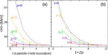
Figure 1: (Color online) Energy expectation values of the $J^{\pi}=0^{+}$ trial wave functions of ⁴⁸Cr in $pf$ shell. (a) the blue, green, purple, and red error bars denote the VMC results with $p=0,1,2,3,$ and $4$, respectively. (b) the blue, green, purple, and red error bars denote the VMC results with $t=0,1,2,3,$ and $4$ as functions of $t+2p$. The lines denote the results of the corresponding $p$-iteration Lanczos method.

Figure 1 also shows the Ritz value of the Lanczos method with $p$-step iterations and $|\psi^{t}\rangle$ being the initial vector. The $p$ and $t$ in Fig.1(a) denote the power $p$ and the number of particle-hole truncation of the wave function $|\psi^{t}\rangle$ in Eq.(1). The exact shell-model energy is $-99.578$MeV, which is almost reached at $p=3,4$ and $t\geq 3$. If the variational parameters of the VMC were determined without statistical error, this trial wave function would equal the wave function obtained by the Lanczos method with $p$-iterations. More generally, this is a Monte Carlo formulation of Krylov subspace technique because the trial wave function is a linear combination of $H^{q}|\psi\rangle$ terms with $0\leq q\leq N$. The VMC results (error bars) agree quite well with those of Lanczos method (lines), which means that the Nelder-Mead optimization with reweighting works quite well. While the energy of the initial state $|\psi^{t}\rangle$, or $p=0$ error bars in Fig.1(a), does not converge well as a function of $t$, the VMC values of $p=3,4$ converges well even for the small $t$.

Since the Hamiltonian only contains two-body interactions, $H^{p}|\psi^{t}\rangle$ is considered to be a state in $(t+2p)$-particle $(t+2p)$-hole truncated subspace. Figure 1(b) shows the energy as a function of $t+2p$. The left ends of these lines on Fig.1(b) correspond to the exact solution with $t$-particle $t$-hole truncation, and therefore the variational lower bound of the truncated subspace. With increasing $p$, the energy converges well and close to the Lanczos value.

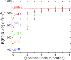
Figure 2: (Color online) B(E2;$0^{+}\rightarrow 2^{+}$) transition probabilities of ⁴⁸Cr provided by the VMC calculations against truncation scheme $t$. The “exact” value is obtained by $t=8$ Lanczos shell-model calculation.

Physical observables other than the energy, e.g. moments and transition probabilities, are also obtained in a similar manner to Ref.vmcsm . Figure 2 shows the B($E2$) transition probability obtained by the VMC. The effective charge is $(e_{p},e_{n})=(1.2,0.8)e$. The convergence behaves similar to the case of the energy in Fig.1(a) and the VMC dramatically improve the $E2$ values in the region of small $t$.

For the demonstration of larger-scale calculations, we discuss the case of ⁶⁰Zn in $pf$ shell with the GXPF1A interaction gxpf1a . The $M$-scheme dimension is huge, $2.2\times 10^{9}$, though it is somehow tractable by the recent shell-model code mshell64 .

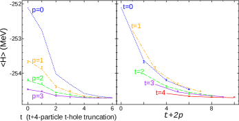
Figure 3: (Color online) Energy expectation values of the $J^{\pi}=0^{+}$ trial wave functions of ⁶⁰Zn in $pf$ shell. See the caption of Fig.1.

Figure 3 shows the energy expectation values of the ground state obtained by the VMC and the corresponding Lanczos method. Though the dimension is about $10^{3}$ times larger than that of ⁴⁸Cr, the energy convergence is similar to Fig.1.

Figure 4: (Color online) Excitation energies of $J^{\pi}=2^{+}$ and $4^{+}$ states of ⁶⁰Zn in $pf$ shell. See the caption of Fig.1.

Figure 4 shows the excitation energies obtained by the VMC approach and corresponding $p$-iterated Lanczos method. The excitation energies converged far faster than the energy itself, and the VMC significantly improves the convergence.

IV Summary

In summary we proposed a new VMC formalism to improve the conventional particle-hole truncation shell-model calculations systematically, and demonstrated its feasibility at ⁶⁰Zn in $pf$ shell. In this formalism, we do not have the sign problem because it is implemented by the variational Monte Carlo, namely the density probability is defined by the wave function squared. However, the power of the Hamiltonian in the Monte Carlo implementation of the Lanczos method is restricted to be rather small, such as $p=3$ or $4$. Nevertheless, it provides us with good convergence of the energy and is expected to be useful to go beyond the conventional diagonalization method. The energy expectation value of our $p$-power VMC scheme agrees with that of $p$-th step Lanczos method in full space within statistical error. It means that the MCMC procedure and reweighting method to determine the variational parameters work well and stable. The present VMC approach provides us with the facile estimation of the exact energy eigenvalue by using the $t$-particle $t$-hole truncated wave functions. The energy variance can also be calculated stochastically with the same formulation, which is expected to be helpful for the energy-variance extrapolation technique variance_extrap , and it remains for future study.

The cache algorithm to store $\langle m|H^{q}|\phi^{t}\rangle$ with a random walker $m$ drastically reduces the computation time At present, since we store all matrix elements on memory, it requires a large amount of memory usage. This difficulty can be eased by sophisticated cache algorithm, the implementation of which is important for further applications.

References

- (1) For review: Z. Bai, Appl. Num. Math. 43, 9 (2002).
- (2) C. Lanczos, J. Res. Nat. Bur. Stand, 45, 255 (1950).
- (3) T. Sebe and J. Nachamkin, Ann. Phys. 51, 100 (1969).
- (4) R.R. Whitehead, Nucl. Phys. A182, 290 (1972).
- (5) J.P. Vary, P. Maris, E. Ng, C. Yang, and M. Sosonkina, J. Phys.: Conf. Ser. 180 012083 (2009).
- (6) M. Horoi, B. A. Brown, T. Otsuka, M. Honma, and T. Mizusaki, Phys. Rev. C 73, 061305(R) (2006).
- (7) C.W. Johnson, S.E. Koonin, G.H. Lang, and W. E. Ormand, Phys. Rev. Lett. 69, 3157 (1992); S. E. Koonin, D. J. Dean, and K. Langanke, Phys. Rep. 278 1, (1997).
- (8) M. A. Rombouts, K. Heyde, and N. Jachowicz, Phys. Rev. Lett. 82 4155 (1999).
- (9) T. Mizusaki and N. Shimizu, Phys. Rev. C 85, 021301(R) (2012).
- (10) Y. C. Chen and T. K. Lee, Phys. Rev. B 51 6723 (1995).
- (11) S. Sorella, Phys. Rev. B 64, 024512 (2001).
- (12) Numerical Recipes in Fortran 77, the Art of Scientific Computing, 2nd ed., Cambridge University Press: Cambridge, (1992).
- (13) A. M. Ferrenberg and R. H. Swendsen, Phys. Rev. Lett. 61, 2635 (1988), ibid. 63, 1195 (1989).
- (14) M. Honma et al., Eur. Phys. J. A 25, s01, 499 (2005).
- (15) T. Mizusaki, N. Shimizu, Y. Utsuno, and M. Honma, code MSHELL64, unpublished.
- (16) T. Mizusaki and M. Imada, Phys. Rev. C 65, 064319 (2002), ibid; Phys. Rev. C 67, 041301 (2003).