Non-linear and chaotic dynamo regimes

Abstract

An update is given on the current status of solar and stellar dynamos. At present, it is still unclear why stellar cycle frequencies increase with rotation frequency in such a way that their ratio increases with stellar activity. The small-scale dynamo is expected to operate in spite of a small value of the magnetic Prandtl number in stars. Whether or not the global magnetic activity in stars is a shallow or deeply rooted phenomenon is another open question. Progress in demonstrating the presence and importance of magnetic helicity fluxes in dynamos is briefly reviewed, and finally the role of nonlocality is emphasized in modeling stellar dynamos using the mean-field approach. On the other hand, direct numerical simulations have now come to the point where the models show solar-like equatorward migration that can be compared with observations and that need to be understood theoretically.

1 Introduction

The objective of IAU Symposium 294 is to provide an update since IAU Symposium 157 on “The Cosmic Dynamo” in Potsdam, 1992. The title of the present talk reflects the common thinking at that time that nonlinearity and chaos tend to come together. This is highlighted by the realization that a simple mean-field dynamo model for poloidal and toroidal fields needs to be supplemented by a third equation to produce chaos, and the idea that this third equation is the equation of magnetic helicity conservation. These developments have contributed to the unfortunate perception of mean-field dynamo theory being just as a toy rather than a quantitatively predictive theory.

With the advent of numerous computer simulations of hydromagnetic turbulence exhibiting large-scale dynamo action, a new field of computer astrophysics has emerged where the objective is to understand simulated dynamos, where one has a chance to resolve all time and length scales. This approach has helped making mean-field theory quantitatively reliable and predictable.

Various predictions have emerged and have been tested. Firstly, dynamos must transport magnetic helicity to escape catastrophic quenching. They do this through coronal mass ejections and through turbulent exchange across the equator. The resulting field is bi-helical, with opposite signs of magnetic helicity at large and small length scales. The signs depend on the sign of kinetic helicity and on the relative importance of turbulent diffusion. This has meanwhile been confirmed observationally using Ulysses data. Secondly, mean-field theory also predicts the formation of local magnetic flux concentrations as a result of strong density stratification. Simulations have now confirmed this remarkable theoretical prediction. This has opened the floor for suggestions that active regions and sunspots might be shallow phenomena operating near the surface at some 40 Mm depth.

There are also several observations that do not yet have a satisfactory explanation. One of them concerns the dependence of the observed cycle period of late-type stars on their activity and another one is the equatorward migration of toroidal magnetic flux belts during the solar cycle: is it caused by meridional circulation, the migratory properties of the dynamo wave, or something else that we do not know about yet?

2 Dynamo regimes

The graph of the ratio of stellar cycle to rotational frequencies versus magnetic activity or stellar age shows two branches (Brandenburg et al., 1998, hereafter BST); see Figure 1. These branches correspond to active (A) and inactive (I) stars and are separated by what is known as the Vaughan–Preston gap. In addition, there is a third branch of super-active (S) stars (Saar & Brandenburg, 1999). How can we understand the origin of these branches?

Figure 1: BST diagram showing inactive (letters) and active (numbers) stars on separate branches of normalized cycle frequency $\omega_{\rm cyc}/\Omega$ as a function of normalized chromospheric calcium H and K line activity parameter $\langle R^{\prime}_{\rm HK}\rangle$. Approximate age is given on the upper abscissa. As stars evolve, they move along the lower (active) branch toward the left, and then (when the color $B-V$ is between 0.6 and 1.1) jump onto the upper (inactive) branch. Adapted from Brandenburg et al. (1998).

The BST diagram is not just a way of representing the non-dimensional cycle frequency in a two-dimensional diagram, it might represent some deeper physics. In a globally quenched $\alpha\Omega$-type dynamo, i.e., a model where only the smallest wavenumbers have a significant contribution (as found in simulations; see Brandenburg et al., 2008; Rheinhardt & Brandenburg, 2012), the cycle frequency $\omega_{\rm cyc}$ is proportional to $\sqrt{\alpha\Omega^{\prime}}$, where $\alpha$ represents the $\alpha$ effect responsible for reproducing the large-scale magnetic field (Moffatt, 1978; Krause & Rädler, 1980) and $\Omega^{\prime}$ is the radial differential rotation. Both are functions of the angular velocity $\Omega$ (which has been subsumed into a factor $\Omega^{q}$ with a poorly constrained exponent $q$; see BST).

The essential point is that $\omega_{\rm cyc}$ can be regarded as a proxy of $\alpha$. Furthermore, the angular velocity normalized by the turnover time $\tau$, which gives the inverse Rossby number $\mbox{\rm Ro}^{-1}=2\Omega\tau$, can be regarded as a measure of the non-dimensional magnetic field strength, $B/B_{\rm eq}$, where $B_{\rm eq}$ is the equipartition field strength. This is a relationship that is independent of the existence of different branches, i.e., inactive and active stars lie on the same curve (BST). We can therefore imagine the BST diagram being really a representation of $\alpha(B)$, and that the two rising branches describe therefore an anti-quenching of $\alpha$ with $B/B_{\rm eq}$. Indications of this, and a corresponding anti-quenching of the turbulent magnetic diffusivity, have been found in simulations of magneto-buoyancy (Chatterjee et al., 2011). On the other hand, for faster rotation there is a third branch of super-active stars (Saar & Brandenburg, 1999), for which our proxy of $\alpha$ declines with that of $B$.

These considerations are still as exciting today as they were back in 1998, but now we have realistic global simulations of convection that reflect a qualitative leap from earlier work in that we now find for the first time cyclic large-scale dynamo action with equatorward migrating activity belts (Käpylä et al., 2012). One needs to check, however, whether perhaps all of the dynamo solutions obtained so far are representative of the superactive branch, and that the physics behind the active and inactive ones remains still to be discovered. To make progress in understanding the different modes of cyclic stellar activity, one also needs to analyze why those models produce long cycle periods and equatorward migration, both of which are also seen in the Sun, but are theoretically not understood; is it related to the possible dominance of the magnetic $\alpha$ effect (Pouquet et al., 1976) (which is inversely proportional to the density and therefore important near the surface), to the tensorial structure of $\alpha$ ($\alpha_{ij}$) and turbulent diffusion ($\eta_{ijk}$), to meridional circulation, or to subtleties in the differential rotation? Such understanding should be accomplished by deriving and solving suitable mean-field models that reproduce the behavior seen in DNS and Large Eddy Simulations (LES) of the Sun.

It is unlikely that differences in the cycle period are the only criterion distinguishing stars on the two branches of the evolutionary BST diagram. Surface magnetic field structures as well as their spatio-temporal correlations are now becoming accessible to detailed scrutiny. Quantifying the nature of magnetic fields using observed correlations among the Stokes parameters might help to distinguish different types of behaviors and to associate them with different branches in the BST diagram, which may reflect different underlying dynamo modes. Progress can be made by considering turbulent dynamo simulations at different rotation rates, as has recently been done by Käpylä et al. (2013). We return to this issue in our conclusions and turn attention to recent simulation results that concern the magnetic surface activity of the Sun, such as small-scale or local dynamos and the evidence of helical magnetic fields from the global dynamo.

3 Small-scale and local dynamos

In recent years the action of two separate dynamos in the Sun has become popular; one that governs the 11 year cycle and one that produces the small-scale field of the quiet Sun (Cattaneo, 1999; Cattaneo et al., 2003; Vögler & Schüssler, 2007). This idea is supported by the fact that the observed small-scale field of the Sun is essentially uncorrelated with that of the 11 year cycle (Lites, 2002; Ishikawa & Tsuneta, 2009; Danilovic et al., 2010; Aurière et al., 2010; Stenflo, 2012).

A potential problem is the fact that the critical magnetic Reynolds number $R_{\rm m,{\rm crit}}$ grows larger as one decreases the value of the magnetic Prandtl number, $\mbox{\rm Pr}_{M}=\nu/\eta$, to more realistic values (Schekochihin et al., 2005). Early work of Rogachevskii & Kleeorin (1997) did already predict an increased value of $R_{\rm m,{\rm crit}}$ in the limit of small values of $\mbox{\rm Pr}_{M}$. Boldyrev and Cattaneo (2004) argue that the reason for an increased value of $R_{\rm m,{\rm crit}}$ is connected with the “roughness” of the velocity field. Iskakov et al. (2007) found that $R_{\rm m,{\rm crit}}$ has a local maximum at $\mbox{\rm Pr}_{M}=0.1$, and that it decreases again as $\mbox{\rm Pr}_{M}$ is decreased further. The reason for this is that near $\mbox{\rm Pr}_{M}=0.1$ the resistive wavenumber is about 10 times smaller than the viscous one and thus right within the “bottleneck” where the spectrum is even shallower than in the rest of the inertial range, with a local scaling exponent that corresponds to turbulence that is in this regime rougher still, explaining thus the apparent divergence of $R_{\rm m,{\rm crit}}$.

In the nonlinear regime the magnetic field affects the flow in such a way that the bottleneck effect tends to be suppressed, so the divergence in the roughness disappears and there is a smooth dependence of the saturation field strength on the value of $\mbox{\rm Pr}_{M}$; see Brandenburg (2011) for details. In Figure 2, we show spectra compensated with $\epsilon^{-2/3}k^{5/3}$. For $\mbox{\rm Pr}_{M}=0.02$ and 0.01, the kinetic energy spectra show a clear bottleneck effect, i.e., there is a weak uprise of the compensated spectra toward the dissipative subrange (Falkovich, 1994; Kaneda et al., 2003; Dobler et al., 2003). The compensated magnetic energy spectra peak around $k=20k_{1}$, where $k_{1}=2\pi/L$ is the smallest wavenumber in a domain of size $L$. Both toward larger and smaller values of $k$ there is no clear power-law behavior. The slopes of the $k^{-11/3}$ spectrum of Golitsyn (1960) and Moffatt (1961) and the scale-invariant $k^{-1}$ spectrum (Ruzmaikin & Shukurov, 1982; Kleeorin & Rogachevskii, 1994; Kleeorin et al., 1996) are shown for comparison.

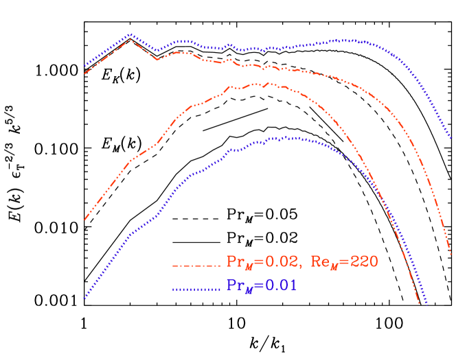
Figure 2: Compensated kinetic and magnetic energy spectra for runs with $\mbox{\rm Pr}_{M}=0.05$, $\mbox{\rm Pr}_{M}=0.02$, and $\mbox{\rm Pr}_{M}=0.01$ for $\mbox{\rm Re}_{M}\approx 160$ as well as one run with $\mbox{\rm Pr}_{M}=0.02$ and $\mbox{\rm Re}_{M}\approx 220$. The resolution is in all cases $512^{3}$ mesh points. The two short straight lines give, for comparison, the slopes $2/3$ (corresponding to a $k^{-1}$ spectrum for $k<20k_{1}$) and $-2$ (corresponding to a $k^{-11/3}$ spectrum for $k>20k_{1}$). Adapted from Brandenburg (2011).

We recall that we have used here the strategy of generating low-$\mbox{\rm Pr}_{M}$ solutions by gradually decreasing $\nu$, and hence increasing the value of Re. As in the case of helical dynamos (Brandenburg, 2009), the fact that a turbulent self-consistently generated magnetic field is present helps reaching these low-$\mbox{\rm Pr}_{M}$ solutions. However, the presence of the magnetic field also modifies the kinetic energy spectrum and makes it decline slightly more steeply than in the absence of a magnetic field; see Figure 2. This suggests that the velocity field would be less rough than in the corresponding case without magnetic fields. Following the reasoning of Boldyrev and Cattaneo (2004), this should make the dynamo more easily excited than in the kinematic case with an infinitesimally weak magnetic field. In other words, there is the possibility of a subcritical bifurcation where the dynamo requires a significantly larger value of $\mbox{\rm Pr}_{M}$ to bifurcate from the trivial $\mbox{\boldmath$B$}{}=\bm{0}$ solution than the value needed to sustain a saturated dynamo.

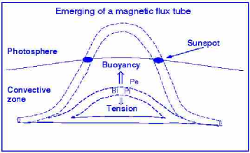
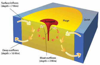
Figure 3: Left: rising flux tube piercing the surface to form a pair of sunspots (taken from http://www.lund.irf.se/helioshome/fluxtube.gif). Right: sunspot with surrounding flow field suggested from local helioseismology. Adapted from Hindman et al. (2009).

4 Solar surface activity

The theory of stellar structure explains that the outer $200\,{\rm Mm}$ of the Sun’s radius are convectively unstable, resulting in fully developed turbulent convection. Numerical simulations of turbulent flows predict that part of the convective kinetic energy is converted to magnetic energy through dynamo action. If we did not have observations, would we have predicted that the Sun’s magnetic field would choose to manifest itself in the form of spots? The answer might well be yes, but perhaps not for the reasons offered in text books. Standard thinking focuses on the tachocline, which is a strong shear layer at the bottom of the convection zone. Strong shear can produce a strong magnetic field in the form of thin flux tubes (Cline et al., 2003; Guerrero & Käpylä, 2011). The magnetic pressure in these tubes expels gas, and so, being less dense than their surrounding, they rise. If a segment of a tube pierces the surface of the Sun, the footpoints of the resulting arch appear as sunspot pairs of opposite polarity (as the magnetic field in the tube has a definite direction; see Figure 3). Simulations, on the other hand, predict turbulent magnetic fields with a diffuse large-scale component throughout the convection zone (Brown et al., 2010; Käpylä et al., 2010; Ghizaru et al., 2010), and this scenario can also reproduce the observed bipolar spots at the surface (Brandenburg, 2005).

It might become possible to use local helioseismology to distinguish between the scenarios sketched in the left and right hand panels of Figure 3. Unlike global helioseismology, local helioseismology is an advanced technique that uses correlations of measured Doppler shifts at the solar surface for different time intervals corresponding to sound travel times for rays down to a given depth, as is seen in the left-hand panel of Figure 4. This technique can provide detailed information on the structure of magnetic fields (Ilonidis et al., 2011) nearby and even inside a sunspot (Kosovichev, 2009). In a particular case, some type of local activity has been detected at a depth of $\sim 60\,{\rm Mm}$, which corresponds to 1/3 of the depth of the convective zone. If this was caused by a rising flux tube, as sketched in Figure 4, one would have expected a wider elongated feature. On the other hand, the observed activity might correspond to signatures of magnetic structures formed by the so-called negative effective magnetic pressure instability (NEMPI, Brandenburg et al., 2011a).

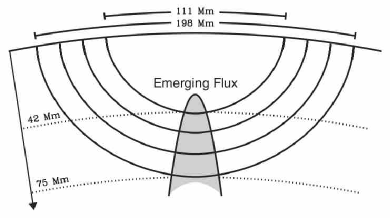
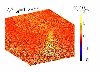
Figure 4: Left: sketch illustrating the detection of subsurface magnetic activity via local helioseismology. Acoustic ray paths are bent back up again because of higher sound speed at greater depth (lower turning points between 42 and 75 Mm are shown). Travel-time anomalies allow detection of emergent flux (sketched in gray) near those turning points. Right: visualization of the magnetic field on the periphery of the computational domain as obtained from NEMPI. Light-yellow regions indicate enhanced flux in a region reminiscent of that implied by local helioseismology (left). Adapted from Ilonidis et al. (2011) [left] and Kemel et al. (2012) [right].

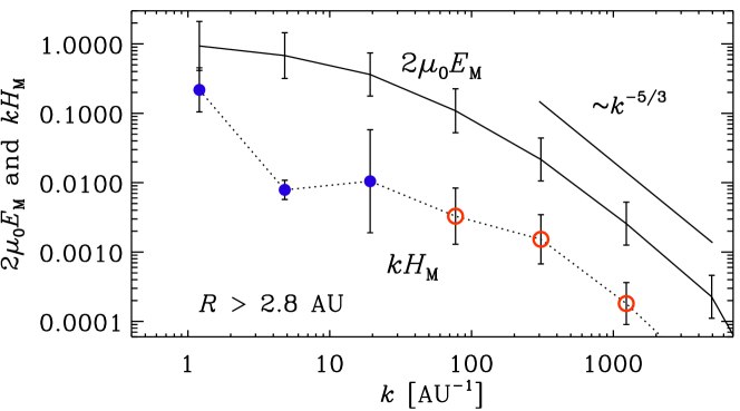
Figure 5: Magnetic energy and helicity spectra, $2\mu_{0}E_{\rm M}(k)$ and $kH_{\rm M}(k)$, respectively, for two separate distance intervals. Furthermore, both spectra are scaled by $4\pi R^{2}$ before averaging within each distance interval above $2.8\,{\rm AU}$. Filled and open symbols denote negative and positive values of $H_{\rm M}(k)$, respectively. Adapted from Brandenburg et al. (2011b).

Coronal mass ejections play a major role in shedding small-scale magnetic helicity from the dynamo to alleviate an otherwise catastrophic quenching of the dynamo (Blackman & Brandenburg, 2003). Meanwhile, models have made contact with unexpected phenomena taking place in the solar wind. A striking example is the sign reversal of small-scale magnetic helicity away from the Sun. This surprising result was first obtained by analyzing data from the Ulysses spacecraft (Brandenburg et al., 2011b), see Figure 5, but the interpretation was greatly aided by similar results from simulations of Warnecke et al. (2011). It now seems that the reason for this is an essentially turbulent-diffusive transport down the local gradient of magnetic magnetic helicity density – even in the wind (Warnecke et al., 2012). While this work has focussed on parameter studies exploring the conditions for plasmoid ejections from helically forced turbulence as well as rotating convection, the physical realism of the model remained poor. The density contrast between dynamo region and corona is much bigger in reality, see for example Pinto et al. (2011). Significant improvements are possible with only modest increase of numerical resolution, as has been shown by Bingert & Peter (2011) using Pencil Code simulations with a realistic setup. One may envisage important follow-up diagnostics by producing visualizations of helical magnetic fields in the corona (see the left-hand panel of Figure 6) and to compute cases in which the field is generated either self-consistently by a dynamo beneath the surface, as in Warnecke et al. (2011, 2013), or the field is injected as a twisted flux tube in a deeper layer and let to emerge at the surface. Simulations without shear have successfully produced twisted magnetic field lines from a self-consistently generated bipolar sheet (see middle panel of Figure 6), but this has not yet been attempted in simulations where more localized bipolar regions are produced. An example of the formation of such regions has been seen in dynamo simulations with strong shear (Brandenburg, 2005) leading to the occasional formation of bipolar regions when opposite polarities can be drawn apart by latitudinal differential rotation; see the right-hand panel of Figure 6. Observational evidence for such a process has been provided by Kosovichev & Stenflo (2008).

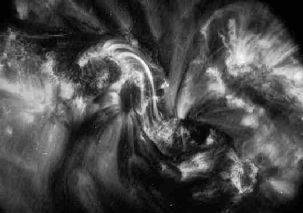
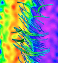
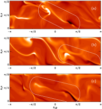
Figure 6: Left: twisted magnetic field lines from a bipolar region on the Sun, as seen in X-rays (adapted from Gibson et al., 2002). Middle: twisted magnetic field lines from a self-consistently generated bipolar sheet (Warnecke & Brandenburg, 2010), not a bipolar region. Here the field is generated by a dynamo without shear. Right: bipolar regions as seen in simulations with shear (Brandenburg, 2005). Light (dark) shades correspond to positive (negative) line of sight magnetic field. Adapted from Gibson et al. (2002) [left], Warnecke & Brandenburg (2010) [middle], and Brandenburg (2005) [right].

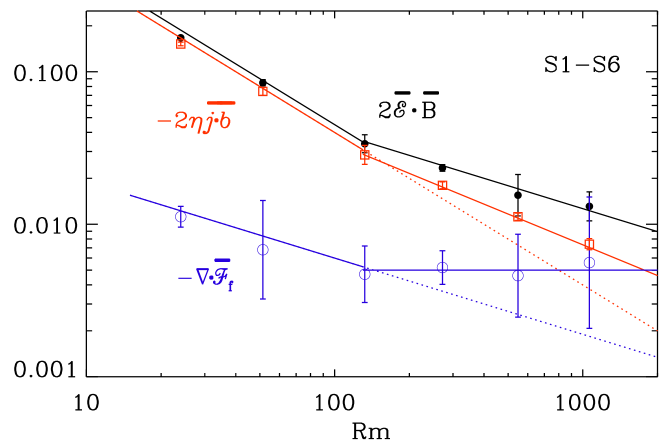
Figure 7: Scaling properties of the vertical slopes of $2\overline{\mbox{\boldmath${\cal E}$}}{}\cdot\overline{\mbox{\boldmath$B$}}{}$, $-2\eta\mu_{0}\,\overline{\mbox{\boldmath$j$}{}\cdot\bm{b}}$, and $-\mbox{\boldmath$\nabla$}{}\cdot\overline{\mbox{\boldmath$F$}}_{\rm f}{}$. The three quantities vary approximately linearly with $z$, so the three labels indicate their non-dimensional values at $k_{1}z=1$. Adapted from Del Sordo et al. (2013).

Recent work using a simple model with a galactic wind has shown, for the first time, that shedding magnetic helicity by fluxes may indeed be possible. We recall that the evolution equation for the mean magnetic helicity density of fluctuating magnetic fields, $\overline{h}_{\rm f}=\overline{\mbox{\boldmath$a$}{}\cdot\bm{b}}$, is

$${\partial\overline{h}_{\rm f}\over\partial t}=-2\overline{\mbox{\boldmath${\cal E}$}}{}\cdot\overline{\mbox{\boldmath$B$}}{}-2\eta\mu_{0}\,\overline{\mbox{\boldmath$j$}{}\cdot\bm{b}}-\mbox{\boldmath$\nabla$}{}\cdot\overline{\mbox{\boldmath${\cal F}$}}_{\rm f}{},$$ (1)

where we allow two contributions to the flux of magnetic helicity from the fluctuating field $\overline{\mbox{\boldmath${\cal F}$}}_{\rm f}{}$: an advective flux due to the wind, $\overline{\mbox{\boldmath${\cal F}$}}_{\rm f}{}^{\rm w}=\overline{h}_{\rm f}\overline{\bm{U}}_{\rm w}$, and a turbulent–diffusive flux due to turbulence, modelled here by a Fickian diffusion term down the gradient of $\overline{h}_{\rm f}$, i.e., $\overline{\mbox{\boldmath${\cal F}$}}_{\rm f}{}^{\rm diff}=-\kappa_{h}\mbox{\boldmath$\nabla$}{}\overline{h}_{\rm f}$. Here, $\overline{\mbox{\boldmath${\cal E}$}}{}=\overline{\mbox{\boldmath$u$}{}\times\bm{b}}$ is the electromotive force of the fluctuating field. The scaling of the terms on the right-hand side with $\mbox{\rm Re}_{M}$ has been considered before by Mitra et al. (2010) and Hubbard & Brandenburg (2010).

In Figure 7 we show the basic result of Del Sordo et al. (2013). As it turns out, below $\mbox{\rm Re}_{M}=100$ the $2\eta\mu_{0}\overline{\mbox{\boldmath$j$}{}\cdot\bm{b}}$ term dominates over $\mbox{\boldmath$\nabla$}{}\cdot\overline{\mbox{\boldmath${\cal F}$}}_{\rm f}{}$, but because of the different scalings (slopes being $-1$ and $-1/2$, respectively), the $\mbox{\boldmath$\nabla$}{}\cdot\overline{\mbox{\boldmath${\cal F}$}}_{\rm f}{}$ term is expected to become dominant for larger values of $\mbox{\rm Re}_{M}$ (about 3000). Surprisingly, however, $\mbox{\boldmath$\nabla$}{}\cdot\overline{\mbox{\boldmath${\cal F}$}}_{\rm f}{}$ becomes approximately constant for $\mbox{\rm Re}_{M}\mathrel{\mathchoice{\vbox{\offinterlineskip\halign{\hfil$\displaystyle#$\hfil\cr>\cr\sim\cr}}}{\vbox{\offinterlineskip\halign{\hfil$\textstyle#$\hfil\cr>\cr\sim\cr}}}{\vbox{\offinterlineskip\halign{\hfil$\scriptstyle#$\hfil\cr>\cr\sim\cr}}}{\vbox{\offinterlineskip\halign{\hfil$\scriptscriptstyle#$\hfil\cr>\cr\sim\cr}}}}100$ and $2\eta\mu_{0}\overline{\mbox{\boldmath$j$}{}\cdot\bm{b}}$ shows now a shallower scaling (slope $-1/2$). This means that that the two curves would still cross at a similar value. Our data suggest, however, that $\mbox{\boldmath$\nabla$}{}\cdot\overline{\mbox{\boldmath${\cal F}$}}_{\rm f}{}$ may even rise slightly, so the crossing point is now closer to $\mbox{\rm Re}_{M}=1000$.

We have mentioned above some surprising behavior that has been noticed in connection with the small-scale magnetic helicity flux in the solar wind. Naively, if negative magnetic helicity from small-scale fields is ejected from the northern hemisphere, one would expect to find negative magnetic helicity at small scales anywhere in the exterior. However, if a significant part of this wind is caused by a diffusive magnetic helicity flux, this assumption might be wrong and the sign changes such that the small-scale magnetic helicity becomes positive some distance away from the dynamo regime. In Figure 8 we reproduce in graphical form the explanation offered by Warnecke et al. (2012).

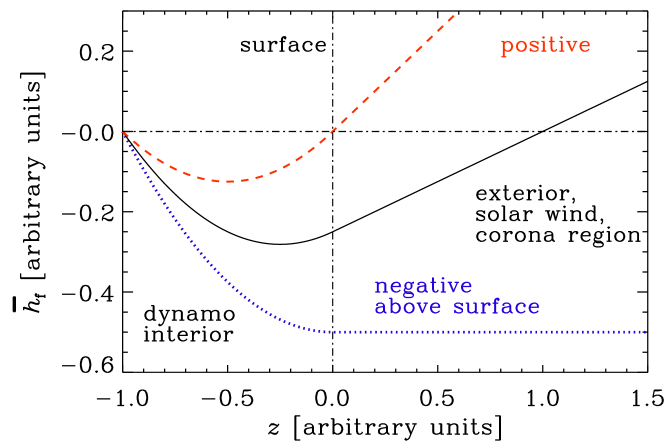
Figure 8: Sketch showing possible solutions $\overline{h}_{\rm f}(z)$ (upper panel) with $S={\rm const}{}=-1$ in $z<0$ and $S=0$ in $z>0$. The red (dashed) and black (solid) lines show solutions for which the magnetic helicity flux ($-\kappa_{h}{\rm d}{}\overline{h}_{\rm f}/{\rm d}{}z$, see lower panel) is negative in the exterior. This corresponds to the case observed in the Sun. The blue (dotted) line shows the case, where the magnetic helicity flux is zero above the surface and therefore do not reverse the sign of $\overline{h}_{\rm f}(z)$ in the exterior. Adapted from Warnecke et al. (2012).

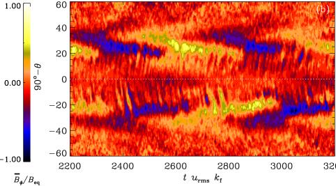
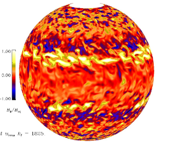
Figure 9: Left: azimuthally averaged toroidal magnetic field as a function of time (in turnover times) and latitude (clipped between $\pm 60^{\circ}$). Note that on both sides of the equator ($90^{\circ}-\theta=\pm 25^{\circ}$), positive (yellow) and negative (blue) magnetic fields move equatorward, but the northern and southern hemispheres are slightly phase shifted relative to each other. Right: Snapshot of the toroidal magnetic field $B_{\phi}$ at $r=0.98$ outer radii. Adapted from Käpylä et al. (2012).

5 Conclusions and further remarks

In this review we have put emphasis on the appearance of magnetic helicity at and above the surface of the dynamo. Other important diagnostics may come from local helioseismology to distinguish between shallow and deeply rooted dynamo scenarios. As mentioned above, simulations by various groups all produce distributed dynamo action where the magnetic field is present throughout the convection zone.

A major breakthrough has been achieved through the recent finding of equatorward migration of magnetic activity belts in the course of the cycle (Käpylä et al., 2012); see Figure 9. These results are robust and have now been reproduced in extended simulations that include a simplified model of an outer corona (Warnecke et al., 2013). Interestingly, the convection simulations of other groups produce cycles only at rotation speeds that exceed those of the present Sun by a factor of 3–5 (Brown et al., 2011); see also Racine et al. (2011) for recent cyclic models at solar rotation speeds. Both lower and higher rotation speeds give, for example, different directions of the dynamo wave (Käpylä et al., 2012). Different rotation speeds correspond to different stellar ages (from 0.5 to 8 gigayears for rotation periods from 10 to 40 days), because magnetically active stars all have a wind and are subject to magnetic braking (Skumanich, 1972). In addition, all simulations are subject to systematic “errors” in that they poorly represent the small scales and emulate in that way an effective turbulent viscosity and magnetic diffusivity that is larger than in reality; see the corresponding discussion in Sect. 4.3.2 of Brandenburg et al. (2012) in another context. In future simulations, it will therefore be essential to explore the range of possibilities by including stellar age as an additional dimension of the parameter space.

In future work it will be important to understand the results of simulations using simpler mean-field models. A potential problem is the fact that the turbulent eddies often have sizes comparable with the size of the domain. In that case, scale separation in space or time is poor and the mean-field $\alpha$ effect and turbulent diffusivity have to be replaced by integral kernels by which the dependence of the mean electromotive force on the mean magnetic field becomes nonlocal.

In Figure 10 we show results for the Fourier transformed integral kernels $\tilde{\alpha}(k)$ and $\tilde{\eta}_{\rm t}(k)$. Both $\tilde{\alpha}$ and $\tilde{\eta}_{\rm t}$ decrease monotonously with increasing $|k|$. The two values of $\tilde{\alpha}$ for a given $k/k_{\rm f}$ but different $k_{\rm f}/k_{1}$ and $\mbox{\rm Re}_{M}$ are always very close together. The functions $\tilde{\alpha}(k)$ and $\tilde{\eta}_{\rm t}(k)$ are well represented by Lorentzian fits of the form

$$\tilde{\alpha}(k)={\alpha_{0}\over 1+(k/k_{\rm f})^{2}}\,,\quad\tilde{\eta}_{\rm t}(k)={\eta_{\rm t0}\over 1+(k/2k_{\rm f})^{2}}\,.$$ (2)

In Figure 10 we show the kernels $\hat{\alpha}(\zeta)$ and $\hat{\eta}_{\rm t}(\zeta)$ obtained numerically. Observationally, similar results have been obtained by Abramenko et al. (2011).

Figure 10: Left: Dependences of the normalized $\tilde{\alpha}$ and $\tilde{\eta}_{\rm t}$ on the normalized wavenumber $k/k_{\rm f}$ for isotropic turbulence forced at wavenumbers $k_{\rm f}/k_{1}=5$ with $\mbox{\rm Re}_{M}=10$ (squares) and $k_{\rm f}/k_{1}=10$ with $\mbox{\rm Re}_{M}=3.5$ (triangles). The solid lines give the Lorentzian fits (2). Right: Normalized integral kernels $\hat{\alpha}$ and $\hat{\eta}_{\rm t}$ versus $k_{\rm f}\zeta$ for isotropic turbulence forced at wavenumbers $k_{\rm f}/k_{1}=5$ with $\mbox{\rm Re}_{M}=10$ (squares) and $k_{\rm f}/k_{1}=10$ with $\mbox{\rm Re}_{M}=3.5$ (triangles). Adapted from Brandenburg et al. (2008).

The results presented in Figure 10 show no noticeable dependencies on $\mbox{\rm Re}_{M}$. Although we have not performed any systematic survey in $\mbox{\rm Re}_{M}$, we interpret this as an extension of the above–mentioned results of Sur et al. (2008) for $\alpha$ and $\eta_{\rm t}$ to the integral kernels $\hat{\alpha}$ and $\hat{\eta}_{\rm t}$. Of course, this should also be checked with higher values of $\mbox{\rm Re}_{M}$. Particularly interesting would be a confirmation of different widths for the profiles of $\hat{\alpha}$ and $\hat{\eta}_{\rm t}$.

The challenge in solar and stellar dynamo theory is nowadays not just the understanding of the nature and origin of magnetic fields in observed stars and in the Sun, but also the understanding of simulated dynamos. Here we have a clear chance in achieving one-to-one agreement because the magnetic Reynolds numbers are still manageable. Only when such agreement has been achieved will we be able to address in a meaningful way solar and stellar dynamos.