Avoiding Death by Vacuum

Abstract

The two-Higgs doublet model (2HDM) can have two electroweak breaking, CP-conserving, minima. The possibility arises that the minimum which corresponds to the known elementary particle spectrum is metastable, a possibility we call the “panic vacuum”. We present analytical bounds on the parameters of the softly broken Peccei-Quinn 2HDM which are necessary and sufficient conditions to avoid this possibility. We also show that, for this particular model, the current LHC data already tell us that we are necessarily in the global minimum of the theory, regardless of any cosmological considerations about the lifetime of the false vacua.

1 Introduction

The two Higgs doublet model [1] is one of the simplest extensions of the Standard Model (SM) of particle physics. It has the particle content of the SM plus a second Higgs doublet, of the same hypercharge as the SM’s. It has a very rich phenomenology (for a review, see [2]), including the possibility of spontaneous CP-violation, dark matter candidates and a richer scalar spectrum, including two CP-even scalars (usually denoted $h$ and $H$), a pseudoscalar ($A$) and a charged scalar ($H^{\pm}$). With the recent discovery of the Higgs boson [3, 4], and a possibility that its observed properties might exhibit some deviations from its expected SM behaviour, it is interesting to look into SM extensions and compare their predictions with data. In that regard, the 2HDM has already shown to be able to do a good job describing current LHC results [5, 6, 7, 8].

The 2HDM also has a very rich vacuum structure: unlike the SM, there is the possibility of occurrence of charge breaking vacua which would give mass to the photon; and, as already mentioned, there is also the possibility of vacua which, other than the electroweak symmetry, also boasts a spontaneous breaking of the CP symmetry. It has been proven [9, 10], though, that whenever a vacuum which breaks electroweak symmetry but preserves the electromagnetic and CP symmetries exists - which we call a “normal” vacuum - any charge or CP breaking stationary points which might exist are necessarily saddle points, and lie above the normal minimum. The stability of the normal minimum against charge or CP breaking is thus guaranteed. There is however another possibility: the 2HDM potential, under certain circumstances, can have two normal minima, which coexist with one another [11, 12, 13]. In one of those minima, the two Higgs doublets, $\Phi_{1}$ and $\Phi_{2}$, would have vacuum expectation values (vevs) $v_{1}$ and $v_{2}$ such that $v_{1}^{2}+v_{2}^{2}\,=\,246$ GeV², and all elementary particles would have the masses we know - this would be “our” minimum. But in the second minimum - deeper or higher than ours - the fields would have vevs $\{v^{\prime}_{1}\,,\,v^{\prime}_{2}\}$, with ${v^{\prime}}^{2}_{1}\,+\,{v^{\prime}}^{2}_{2}\,\neq 246$ GeV² - and the elementary particles might have masses much smaller, or larger, than what is observed.

The possibility then arises that “our” vacuum is not the global minimum of the theory - and the universe would therefore be in a metastable state, with the possibility of tunneling to the deeper vacuum. We call this situation the “panic vacuum”. It is therefore interesting to ascertain: under what conditions such vacua might occur; whether the current experimental data can tell us something about the nature of the vacuum in the 2HDM; what regions of parameter space are free of these panic vacua. In [14] we presented the conditions that the parameters of the potential need to obey so one can avoid the presence of a panic vacuum in the softly broken Peccei-Quinn [15] version of the 2HDM. In this talk, we will briefly review those theoretical bounds, as well as the phenomenological analysis that was performed to compare the model’s predictions with the current LHC data.

2 Panic vacuum bounds in the softly broken Peccei-Quinn 2HDM

The most general 2HDM scalar potential has, after all possible simplifications, 11 independent real parameters. But it is plagued by tree-level flavour-changing neutral currents (FCNC) on the Higgs Yukawa interactions, which are extremely constrained by experimental observations. To evade this problem - and increase the predictive power of the theory, by reducing the number of free parameters - one usually imposes a symmetry on the Lagrangian. One such example is the discrete $Z_{2}$ symmetry, $\Phi_{1}\rightarrow\Phi_{1}$ and $\Phi_{2}\rightarrow-\Phi_{2}$, first proposed by Glashow, Weinberg and Paschos [16, 17]. Another possibility is to impose a global, continuous $U(1)$ symmetry, $\Phi_{1}\rightarrow\Phi_{1}$ and $\Phi_{2}\rightarrow\,e^{i\alpha}\Phi_{2}$, for any real value of $\alpha$. This symmetry also liquidates any tree-level FCNC but, if broken by the vacuum (which occurs if both scalar fields develop a vev), leads to a massless pseudoscalar, an axion. To prevent that one adds a real soft breaking term to the potential, thus obtaining an acceptable scalar spectrum.

The softly broken Peccei-Quinn potential is then written as

$$V = m_{11}^{2}\Phi_{1}^{\dagger}\Phi_{1}+m_{22}^{2}\Phi_{2}^{\dagger}\Phi_{2}-m_{12}^{2}\left[\Phi_{1}^{\dagger}\Phi_{2}+\Phi_{2}^{\dagger}\Phi_{1}\right]$$ (1)

$$+\frac{1}{2}\lambda_{1}(\Phi_{1}^{\dagger}\Phi_{1})^{2}+\frac{1}{2}\lambda_{2}(\Phi_{2}^{\dagger}\Phi_{2})^{2}+\lambda_{3}(\Phi_{1}^{\dagger}\Phi_{1})(\Phi_{2}^{\dagger}\Phi_{2})+\lambda_{4}(\Phi_{1}^{\dagger}\Phi_{2})(\Phi_{2}^{\dagger}\Phi_{1}),$$

where all the parameters are real and the soft breaking term is $m_{12}^{2}$. It can be seen [11, 12, 13] that this model, due precisely to the soft breaking term, can have two normal minima. If the the potential has a depth equal to $V_{N}$ in the minimum with vevs $\{v_{1}\,,\,v_{2}\}$, and a depth $V_{N^{\prime}}$ in the minimum with vevs $\{v^{\prime}_{1}\,,\,v^{\prime}_{2}\}$, it is possible to show that

$$V_{N^{\prime}}-V_{N} = \frac{1}{4}\,\left[\left(\frac{m^{2}_{H^{\pm}}}{v^{2}}\right)_{N}-\left(\frac{m^{2}_{H^{\pm}}}{v^{2}}\right)_{N^{\prime}}\right]\,(v_{1}v^{\prime}_{2}-v_{2}v^{\prime}_{1})^{2}$$ (2)

$$= \frac{m^{2}_{12}}{4v_{1}v_{2}}\,\left(1-\frac{v_{1}v_{2}}{v^{\prime}_{1}v^{\prime}_{2}}\right)\,(v_{1}v^{\prime}_{2}-v_{2}v^{\prime}_{1})^{2}\,$$

with both the charged Higgs mass $m^{2}_{H^{\pm}}$ and the sum of the squared vevs $v^{2}$ being computed at each of the minima. It is not therefore obvious which is the deepest minimum.

In refs. [12, 13, 18] generic conditions for the existence of two minima in the 2HDM were established, being put into a simpler form in [14]. Thus it is possible to show that the Peccei-Quinn potential can have two normal minima if the following conditions are met:

$$m_{11}^{2}+k^{2}\,m_{22}^{2} < 0,$$ (3)

$$\sqrt[3]{x^{2}}+\sqrt[3]{y^{2}} \leq 1,$$ (4)

where the variables $x$ and $y$ are given by

$$x = \frac{4\ k\ m_{12}^{2}}{m_{11}^{2}+k^{2}\,m_{22}^{2}}\,\frac{\sqrt{\lambda_{1}\lambda_{2}}}{\lambda_{34}-\sqrt{\lambda_{1}\lambda_{2}}},$$

$$y = \frac{m_{11}^{2}-k^{2}\,m_{22}^{2}}{m_{11}^{2}+k^{2}\,m_{22}^{2}}\,\frac{\sqrt{\lambda_{1}\lambda_{2}}+\lambda_{34}}{\sqrt{\lambda_{1}\lambda_{2}}-\lambda_{34}},$$ (5)

and we have defined

$$\lambda_{34}=\lambda_{3}+\lambda_{4}\hskip 14.22636pt\textrm{and}\hskip 14.22636ptk=\sqrt[4]{\frac{\lambda_{1}}{\lambda_{2}}}.$$ (6)

The curve $\sqrt[3]{x^{2}}+\sqrt[3]{y^{2}}=1$, which delimits the region of parameter space where two minima can occur, is known as an astroid. To verify whether the $\{v_{1}\,,\,v_{2}\}$ minimum is the global one, one simply has to verify if the following condition is met: one computes, at that minimum, the value of the following quantity, which we dub the “discriminant”,

$$D\,=\,\left(m_{11}^{2}-k^{2}m_{22}^{2}\right)(\tan{\beta}-k).$$ (7)

Our minimum is the global one if, and only if, $D\,>\,0$. This condition can be verified regardless of eqs. 3, 4. Meaning, we do not even need to know whether the potential has two minima, this extremely simple condition is all we need to check to ascertain the nature of the 2HDM minimum.

3 LHC data and panic vacua

In order to verify how often the possibility of two minima arises in the Peccei-Quinn potential, we performed a thorough scan of the model’s parameter space. To wit, we have considered $m_{h}=125$ GeV, $125<m_{H}<900$ GeV, $90<m_{A},m_{H^{\pm}}<900$ GeV, $-\pi/2<\alpha<\pi/2$, $1<\tan\beta<40$ and $|m^{2}_{12}|<900$ GeV². So that the potential is bounded from below, the quartic couplings of the potential must obey

$$\lambda_{1}>0 \lambda_{2}>0\;,$$ ,

$$\lambda_{3}>-\sqrt{\lambda_{1}\lambda_{2}} \lambda_{3}+\lambda_{4}-|\lambda_{5}|>-\sqrt{\lambda_{1}\lambda_{2}}\;.$$ , (8)

We further demanded that the quartic couplings be such that the model satisfies perturbative unitarity [19, 20] and the electroweak precision constraints stemming from the S, T and U parameters [21, 22, 23, 24]. All of these bounds apply to the theory’s scalar sector. But the $U(1)$ symmetry we imposed, even though softly broken, needs to be a symmetry of the full Lagrangian, otherwise we would end up with a non-renormalizable model. There are several ways to extend this symmetry from the scalar to the fermion sector. Here we will consider the two most studied: Model I, where the fermion fields transform under the global $U(1)$ in such a way that only $\Phi_{2}$ couples to the fermions; and Model II, where $\Phi_{2}$ couples only to up-type quarks, and $\Phi_{1}$ to down-type quarks and charged leptons. Both of these models possess very different phenomenologies. Also, data stemming from B-physics measurements put severe constraints on each of them. We have taken those bounds into account, incorporating them in our simulations [25, 26].

The relevance of the conditions 3- 4 can be appreciated in figure 1. For the totality of the parameter space we scanned, we plot,

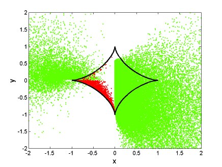
Figure 1: Distribution of generated points in the $x$ and $y$ variables. The dark curve is the astroid described by eq. 4. Points inside that curve can have two minima. The red/dark grey points shown here correspond to panic vacua. The green/light grey points correspond to either the non-existence of two minima, or the case where our vacuum is the global one.

in the $\{x\,,\,y\}$ plane of the variables defined in eq. 5, the points which correspond to the panic vacua situation (in red/dark grey) and those for which our minimum is “safe” - whether because there is a single minimum, or because the second minimum is above ours. The point we wish to stress is that the occurrence of panic vacua is not a curiosity of the model: for a blind scan of the parameter space, obeying all reasonable constraints, a very large quantity of points with panic vacua appears.

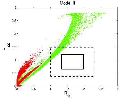
Figure 2: $R_{ZZ}$ versus $R_{\gamma\gamma}$ for Model II. We show rough 1-$\sigma$ (solid line) and 2-$\sigma$ (dashed line) current bounds obtained from LHC data. Green/light grey points are the totality of our simulation; red/dark grey points correspond to panic vacua.

We then use the generated points to compute $R_{f}$, defined as the number of events predicted in the 2HDM for the process $pp\rightarrow h\rightarrow f$, for some final state $f$, divided by the prediction obtained in the SM for the same final state. Current LHC bounds at $1\sigma$, which we took from [27], are $R_{ZZ}=0.93\pm 0.28$, $R_{\gamma\gamma}=1.66\pm 0.33$. We sum over all production mechanisms, such as gluon-gluon fusion, vector boson fusion (VBF), associated Higgs production (with a gauge boson or a $t\bar{t}$ pair) or $b\bar{b}$ fusion. In fig. 2 we show, for Model II, the observables $R_{ZZ}$ versus $R_{\gamma\gamma}$, where the points corresponding to panic vacua are shown in red/dark grey. We see that Model II is capable, at the 2-$\sigma$ level, to obey current experimental bounds. However, even at that level, all points corresponding to panic vacua are disfavoured by current bounds - remarkably, even though the LHC hasn’t found (yet) any evidence for more than one scalar, the current data is already capable of telling us a lot about the vacuum structure of the 2HDM. We see that this

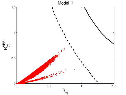
Figure 3: $R^{VBF}_{\gamma\gamma}$ versus $R_{\gamma\gamma}$ for Model II. We show rough 1-$\sigma$ (solid line) and 2-$\sigma$ (dashed line) current bounds obtained from LHC data. The red/dark grey points correspond to panic vacua.

trend is also verified in other variables, such as those plotted in fig. 3. There we plot the Higgs $\gamma\gamma$ event rate (relative to the SM’s), produced only via the VBF mechanism versus its total production rate. We only show those points corresponding to the panic vacuum solutions, and see that, even at the 2-$\sigma$ level, they are strongly disfavoured.

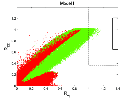
Figure 4: $R_{ZZ}$ versus $R_{\gamma\gamma}$ for Model I. We show rough 1-$\sigma$ (solid line) and 2-$\sigma$ (dashed line) current bounds obtained from LHC data. Green/light grey points are the totality of our simulation; red/dark grey points correspond to panic vacua.

The same, however, cannot be said to occur in Model I. Even though, as we see in fig. 4, where we once again plot $R_{ZZ}$ versus $R_{\gamma\gamma}$, all panic points (the red/dark grey ones) lie outside even the 2-$\sigma$ band, in the $R^{VBF}_{\gamma\gamma}$-$R_{\gamma\gamma}$ plane that would not occur: the 2-$\sigma$ band would include some panic points, even though that would not occur at the 1-$\sigma$ level. Of course, the fact that all panic points are excluded due to the results of fig. 4 would mean that for Model I, as well, the existence of panic vacua is strongly disfavoured by current LHC data, albeit perhaps less so than in Model II.

4 Conclusions

The 2HDM can have metastable neutral vacua, and this raises the possibility that the minimum we are currently inhabiting could not be the global minimum of the model. We have presented the extremely simple conditions one has to impose on the parameters of the potential to prevent this situation. They are, we believe, to be taken as seriously as the bounded-from-below conditions one usually imposes on the potential, or those enforcing perturbative unitarity. These bounds can also be extended to other versions of the 2HDM, and that work is underway [28].

The argument can be made that the existence of a metastable vacuum is not a problem per se, if the tunneling time from the false vacuum to the true one is larger than the current age of the universe. We have performed a quick estimate of the lifetimes of our panic vacua, and concluded that most of them would have lifetimes inferior to the age of the universe, therefore they would correspond to truly undesirable regions of parameter space, in disagreement with observed phenomenology.

But the most interesting aspect of our analysis, we believe, is the fact that, regardless of any calculation of vacuum lifetimes - and it must be stressed that that calculation is rife with approximations and considerable assumptions - the current data stemming from the LHC already permit us to conclude a lot about the nature of our vacuum, if Nature is indeed described by the 2HDM. Namely, the present LHC bounds on several observables already tells us to strongly disfavour the possibility that the vacuum we are in is not the global minimum of the theory. But that does not diminish the validity of the panic vacuum bounds we presented here, nor their interest: for we see that panic vacua occur for perfectly ordinary values of the 2HDM parameters, which predict values for observables which are not a priori absurd. And in any case, we see that the discriminant of eq. 7, by itself, allows us to obtain information, via only particle physics experiments, about a very interesting cosmological subject: the nature of the universe’s vacuum.

The works of A.B., P.M.F. and R.S. are supported in part by the Portuguese Fundação para a Ciência e a Tecnologia (FCT) under contract PTDC/FIS/117951/2010, by FP7 Reintegration Grant, number PERG08-GA-2010-277025, and by PEst-OE/FIS/UI0618/2011. The work of J.P.S. is funded by FCT through the projects CERN/FP/109305/2009 and U777-Plurianual, and by the EU RTN project Marie Curie: PITN-GA-2009-237920. I.P.I. is thankful to CFTC, University of Lisbon, for their hospitality. His work is supported by grants RFBR 11-02-00242-a, RF President grant for scientific schools NSc-3802.2012.2, and the Program of Department of Physics SC RAS and SB RAS ”Studies of Higgs boson and exotic particles at LHC”.

References

References

- [1] T. D. Lee, Phys. Rev. D 8 (1973) 1226.
- [2] G. C. Branco, P. M. Ferreira, L. Lavoura, M. N. Rebelo, M. Sher and J. P. Silva, Phys. Rept. 516, 1 (2012) [arXiv:1106.0034 [hep-ph]].
- [3] G. Aad et al. [ATLAS Collaboration], Phys. Lett. B 716, 1 (2012) [arXiv:1207.7214 [hep-ex]].
- [4] S. Chatrchyan et al. [CMS Collaboration], Phys. Lett. B 716, 30 (2012) [arXiv:1207.7235 [hep-ex]].
- [5] C. -Y. Chen and S. Dawson, arXiv:1301.0309 [hep-ph].
- [6] G. Belanger, B. Dumont, U. Ellwanger, J. F. Gunion and S. Kraml, arXiv:1212.5244 [hep-ph].
- [7] S. Chang, S. K. Kang, J. -P. Lee, K. Y. Lee, S. C. Park and J. Song, with mass around 125 GeV,” arXiv:1210.3439 [hep-ph].
- [8] P. M. Ferreira, R. Santos, M. Sher and J. P. Silva, Phys. Rev. D 85, 077703 (2012) [arXiv:1112.3277 [hep-ph]].
- [9] P. M. Ferreira, R. Santos and A. Barroso, Phys. Lett. B 603 (2004) 219 [Erratum-ibid. B 629 (2005) 114] [arXiv:hep-ph/0406231].
- [10] A. Barroso, P. M. Ferreira and R. Santos, Phys. Lett. B 632 (2006) 684 [arXiv:hep-ph/0507224].
- [11] A. Barroso, P. M. Ferreira and R. Santos, Phys. Lett. B 652 (2007) 181 [arXiv:hep-ph/0702098].
- [12] I. P. Ivanov, Phys. Rev. D 75 (2007) 035001 [Erratum-ibid. D 76 (2007) 039902] [arXiv:hep-ph/0609018].
- [13] I. P. Ivanov, Phys. Rev. D 77 (2008) 015017 [arXiv:0710.3490 [hep-ph]].
- [14] A. Barroso, P. M. Ferreira, I. P. Ivanov, R. Santos and J. P. Silva, arXiv:1211.6119 [hep-ph].
- [15] R. D. Peccei and H. R. Quinn, Phys. Rev. Lett. 38 (1977) 1440.
- [16] S. L. Glashow and S. Weinberg, Phys. Rev. D 15 (1977) 1958.
- [17] E. A. Paschos, Phys. Rev. D 15 (1977) 1966.
- [18] I. P. Ivanov, Phys. Rev. E 79, 021116 (2009).
- [19] S. Kanemura, T. Kubota and E. Takasugi, Phys. Lett. B 313 (1993) 155 [arXiv:hep-ph/9303263].
- [20] A. G. Akeroyd, A. Arhrib and E. -M. Naimi, Phys. Lett. B 490, 119 (2000) [hep-ph/0006035].
- [21] M.E. Peskin and T. Takeuchi, Phys. Rev. D 46, 381 (1992).
- [22] The ALEPH, CDF, D0, DELPHI, L3, OPAL, SLD Collaborations, the LEP Electroweak Working Group, the Tevatron Electroweak Working Group, and the SLD electroweak and heavy flavour Groups, arXiv:1012.2367 [hep-ex].
- [23] M. Baak, M. Goebel, J. Haller, A. Hoecker, D. Ludwig, K. Moenig, M. Schott and J. Stelzer, Eur. Phys. J. C 72, 2003 (2012) [arXiv:1107.0975 [hep-ph]].
- [24] M. Baak, M. Goebel, J. Haller, A. Hoecker, D. Kennedy, R. Kogler, K. Moenig, M. Schott and J. Stelzer, arXiv:1209.2716 [hep-ph].
- [25] T. Hermann, M. Misiak and M. Steinhauser, Next-to-Next-to-Leading Order in QCD,” JHEP 1211 (2012) 036 [arXiv:1208.2788 [hep-ph]].
- [26] F. Mahmoudi, talk given at Prospects For Charged Higgs Discovery At Colliders (CHARGED 2012), 8-11 October, Uppsala, Sweden.
- [27] A. Arbey, M. Battaglia, A. Djouadi and F. Mahmoudi, arXiv:1211.4004 [hep-ph].
- [28] A. Barroso, P. M. Ferreira, I. P. Ivanov and R. Santos, work underway.