Nonadiabatic Van der Pol oscillations in molecular transport

Abstract

The force exerted by the electrons on the nuclei of a current-carrying molecular junction can be manipulated to engineer nanoscale mechanical systems. In the adiabatic regime a peculiarity of these forces is negative friction, responsible for Van der Pol oscillations of the nuclear coordinates. In this work we study the robustness of the Van der Pol oscillations against high-frequency bias and gate voltage. For this purpose we go beyond the adiabatic approximation and perform full Ehrenfest dynamics simulations. The numerical scheme implements a mixed quantum-classical algorithm for open systems and is capable to deal with arbitrary time-dependent driving fields. We find that the Van der Pol oscillations are extremely stable. The nonadiabatic electron dynamics distorts the trajectory in the momentum-coordinate phase space but preserves the limit cycles in an average sense. We further show that high-frequency fields change both the oscillation amplitudes and the average nuclear positions. By switching the fields off at different times one obtains cycles of different amplitudes which attain the limit cycle only after considerably long times.

I Introduction

Research activity on the interaction between electrons and nuclei began more than a century ago, and still today continues to stimulate new ideas and to pose challenging problems. Some of the open issues in this field go back to the early studies by Peierls on one-dimensional lattice instabilities,peierls to continue with the works of Feynman, Frölich and Holstein on polarons,mahan the study of charge and heat conduction,ziman to arrive to present day open questions about the role of phonons in superconductivity/magnetism for layered structures,dagotto to mention a few significative examples. Modern research covers also more fundamental aspects. The electron-nuclei interaction (ENI) coupling is typically derived from the potential energy surfaces of the Born-Oppenheimer approximation. As the coupling relies on an approximation, there has been a significant effort in constructing a formally exact theory. Progress has been made in this context too. The Born-Oppenheimer ansatz for the electron-nuclear wave-function is exact in both the static hunter and time-dependent amg.2010 case and hence the potential energy surfaces constitute a very useful concept even in an exact treatment.

In the last few decades, a more quantitative approach to the understanding of the ENI became possible via computer simulations. For example ab-initio molecular dynamics,cp1985 with a mixed quantum-classical time evolution for electrons and nuclei, was used to study phenomena as different as lattice vibrations and melting, vacancy diffusion, gas-surface dynamics, etc.. Since the advent of nanotechnology, the ENI problem has attracted considerable attention in open nanoscale systems out of equilibrium as well.book2 ; cuevasbook Assessing the nature of ENI and its dependence on the device support in these low-dimensional geometries is a key ingredient to control the decoherence of carriers, the effect of thermal dissipation, in other words to engineer the ENI to increase device efficiency.b2005

While the theoretical study of ENI for steady-state quantum transport has been the subject of large interest, emberly ; ths2001 ; vpl2002 ; bstmo2003 ; ctd.2004 ; cng2004 ; fbjl2004 ; pfb2005 ; fpbj.2007 ; gnr.2007 ; gnr.2008 ; hbt.2009 ; zrsh.2011 ; awmtk.2012 a real-time description of phenomena like, e.g., nuclear rearrangement, multi-stability, electro-migration etc., have received less attention (examples of work done in this less developed area are Refs. [hbf.2004, ; hbfts.2004, ; vsa.2006, ; SSSBHT.2006, ; tb.2011, ]). Recently, the discovery of the nonconservative nature of steady-state forcesdmt.2009 ; tde.2010 has re-awakened the interest in time-dependent phenomena. Two additional types of forces, both linear in the velocity of the nuclear coordinates, have been proposed. One force stems from the friction induced by particle-hole excitations hmzb.2010 ; lhb.2011 and the other force is a Lorentz-like force in which the magnetic field is the curl of the Berry’s vector potential of the Born-Oppenheimer approximation.lbh.2010 All these forces are contained in the Ehrenfest dynamics which evolves the electrons quantum-mechanically in the classical field generated by the nuclei and, at the same time, the nuclear coordinates according to the classical Newton equation in which the forces are generated by the nuclei and the electrons. Assuming that the nuclear motion is slow on the electronic time-scale and that the electrons are fully relaxed in the instantaneous nuclear configuration, one can expand the electronic force in powers of the nuclear velocities (and their derivatives). The zeroth order term corresponds to the nonconservative steady-state force whereas the first-order term corresponds to the sum of the friction force and the Lorentz-like force.bkevo.2011 ; bkevo.2012 We refer to this approximate nuclear dynamics as the Adiabatic Ehrenfest Dynamics (AED). From the explicit expression of the AED forces, either in terms of scattering matrices bkevo.2011 or nonequilibrium Green’s functions,bkevo.2012 one can show that (i) the steady-state force is nonconservative only provided that we are at finite bias and that the number of nuclear degrees of freedom is larger than one, (ii) at zero bias the friction force is always opposite to the nuclear velocity but it can change sign at finite bias (negative friction bc.2006 ; hmzb.2010 ) and (iii) the Lorentz force vanishes if the number of nuclear degrees of freedom is one.

In this work we go beyond the AED by evolving both electrons and nuclei according to the full Ehrenfest dynamics (ED). The ED has so far being employed to study fast vibrational modes in DC regimes.mb.2011 ; npmc.2011 Here, instead, we break the adiabatic condition in a different way. We consider the physical situation of heavy nuclei (and hence slow vibrational modes) and drive the system out of equilibrium by high frequency AC biases or gate voltages. In fact, our scheme can deal with arbitrary driving fields at the same computational cost and is not limited to the wide band limit approximation for the leads. Furthermore, although our scheme can also include several vibrational modes, in this first study we consider only one vibrational mode and focus on one specific issue, namely the negative friction force. The AED predicts the occurrence of limit cycles in the nuclear momentum-coordinate phase space. These cycles are similar to those of a van der Pol oscillator bkevo.2012 and imply that a steady-state is not reached. Is this prediction confirmed by the full ED? What are the qualitative and quantitative differences? How robust are the van der Pol oscillations against ultrafast driving fields? To anticipate our conclusions, we confirm the existence of limit cycles, even though the shape and, more importantly, the period of the oscillations are different from those of the AED. Our main finding, however, is that these cycles are remarkably stable against ultrafast driving fields for which the electrons are far from being relaxed, and hence the AED is not justified. In the next Section we discuss the ED and its adiabatic version. In Section III we introduce the model Hamiltonian with a single vibrational mode and present results on the time-dependent electron current, density and nuclear coordinate. Details on the numerical implementation can be found in Appendix A. Our conclusions and outlook are drawn in Section IV.

II Theoretical framework

We consider a system consisting of a left (L) and right (R) metallic electrode coupled to a central (C) molecular junction. The whole system is initially in the ground state and then driven out of equilibrium by exposing the electrons to an external time-dependent bias $V_{\alpha}(t)$ in lead $\alpha=$L, R and possibly to some time-dependent gate voltage $v_{\rm C}(t)$ in C. We describe the metallic regions L and R by free-electron Hamiltonians

$$\hat{H}_{\alpha}(t)=\sum_{k}(\epsilon_{k\alpha}+V_{\alpha}(t))c^{{\dagger}}_{k\alpha}c_{k\alpha},$$ (1)

with $\alpha={\rm L,R}$. In region C the electrons interact with the classical field generated by the nuclear degrees of freedom ${\bf x}=(x_{1},\ldots,x_{N})$

$$\hat{H}_{\rm C}({\bf x},t)=\sum_{ij=1}^{M}h_{ij}({\bf x},t)c^{{\dagger}}_{i}c_{j},$$ (2)

where the sum runs over the $M$ one-electron states of C. The nuclear Hamiltonian has the general form

$$H_{\rm cl}({\mathbf{p}},{\mathbf{x}})=\sum_{\nu=1}^{N}\frac{p_{\nu}^{2}}{2M_{\nu}}+U_{\rm cl}({\bf x}),$$ (3)

where ${\mathbf{p}}=(p_{1},\ldots,p_{N})$ is canonically conjugated to ${\mathbf{x}}$ and $U_{\rm cl}({\bf x})$ is the classical potential. Finally the metallic electrodes are connected to C through the non-local tunneling operator

$$\hat{H}_{\rm T}=\sum_{\alpha={\rm L,R}}\sum_{ki}\left(T_{k\alpha,i}c^{{\dagger}}_{k\alpha}c_{i}+T^{\ast}_{k\alpha,i}c^{{\dagger}}_{i}c_{k\alpha}\right).$$ (4)

Thus, the full electron Hamiltonian reads

$$\hat{H}_{\rm el}({\mathbf{x}},t)=\hat{H}_{\rm C}({\mathbf{x}},t)+\sum_{\alpha={\rm L,R}}\hat{H}_{\alpha}(t)+\hat{H}_{\rm T}.$$ (5)

II.1 Ehrenfest dynamics

We are interested in calculating time-dependent density, current and nuclear coordinates. In the limit of heavy nuclear masses the nuclear wavefunction is sharply peaked around the classical nuclear coordinates. Then, an expansion around the classical nuclear trajectory leads to a Langevin-type (or stochastic) equation.mb.2011 Ignoring the stochastic forces in this equation corresponds to implement the ED. Denoting by $|\Psi(t)\rangle$ the many-electron state at time $t$, the ED for electrons and nuclei is governed by the equations

$$i\frac{d}{dt}|\Psi(t)\rangle=\hat{H}_{\rm el}({\mathbf{x}}(t),t)|\Psi(t)\rangle,$$ (6)

$$\frac{dx_{\nu}(t)}{dt} = \left[\frac{\partial H_{\rm cl}({\mathbf{p}},{\mathbf{x}})}{\partial p_{\nu}}+\langle\Psi(t)|\frac{\partial\hat{H}_{\rm el}({\mathbf{x}},t)}{\partial p_{\nu}}|\Psi(t)\rangle\right]_{\begin{subarray}{c}{\mathbf{p}}={\mathbf{p}}(t)\\ {\mathbf{x}}={\mathbf{x}}(t)\end{subarray}}$$ (7)

$$= \frac{p_{\nu}(t)}{M_{\nu}},$$

$$\frac{dp_{\nu}(t)}{dt} = -\left[\frac{\partial H_{\rm cl}({\mathbf{p}},{\mathbf{x}})}{\partial x_{\nu}}+\langle\Psi(t)|\frac{\partial\hat{H}_{\rm el}({\mathbf{x}},t)}{\partial x_{\nu}}|\Psi(t)\rangle\right]_{\begin{subarray}{c}{\mathbf{p}}={\mathbf{p}}(t)\\ {\mathbf{x}}={\mathbf{x}}(t)\end{subarray}}$$ (8)

$$= -\frac{\partial U_{\rm cl}({\bf x}(t))}{\partial x_{\nu}}-\sum_{ij}\frac{\partial h_{ij}({\mathbf{x}}(t),t)}{\partial x_{\nu}}\rho_{ji}(t),$$

where in the last equation

$$\rho_{ji}(t)\equiv\langle\Psi(t)|c^{{\dagger}}_{i}c_{j}|\Psi(t)\rangle$$ (9)

is the time-dependent one-particle density matrix. Equations (6-8) are first-order differential equations in time. To solve them we need to specify the boundary conditions. As the system is initially in equilibrium, $|\Psi(0)\rangle=|\Psi_{g}\rangle$ is the electronic ground state, ${\mathbf{x}}(0)={\mathbf{x}}_{g}$ are the ground-state coordinates and ${\bf p}(0)=0$ (we set $t=0$ as the time at which the external bias or gate voltage are switched on). The coordinates ${\bf x}_{g}$ can be calculated from the zero-force equation (see right hand side of Eq. (8))

$$\frac{\partial U_{\rm cl}({\bf x})}{\partial x_{\nu}}=-\sum_{ij}\frac{\partial h_{ij}({\mathbf{x}})}{\partial x_{\nu}}\langle\Psi_{g}|c^{{\dagger}}_{i}c_{j}|\Psi_{g}\rangle.$$ (10)

For $t<0$ the Hamiltonian $\hat{H}_{\rm el}({\bf x},t)$ is a time-independent free-electron Hamiltonian for any ${\mathbf{x}}$ and hence its ground state $\Psi_{g}=\Psi_{g}[{\mathbf{x}}]$ is the Slater determinant formed by the occupied one-electron wavefunctions $\psi_{s}=\psi_{s}[{\mathbf{x}}]$ of energy $\epsilon_{s}=\epsilon_{s}[{\mathbf{x}}]$. Consequently the ground-state density matrix reads

$$\rho_{g,ji}\equiv\langle\Psi_{g}|c^{{\dagger}}_{i}c_{j}|\Psi_{g}\rangle=\sum_{s}^{\rm occ}\psi^{\ast}_{s}(i)\psi_{s}(j)$$ (11)

where $\psi_{s}(i)=\psi_{s}[{\mathbf{x}}](i)$ is the amplitude of $\psi_{s}$ on the $i$-th one-electron state of C. Equations (10,11) constitute a set of coupled equation for the unknown ${\bf x}_{g}$ and $\Psi_{g}$. In Appendix A we describe a numerical procedure to solve these equations for one-dimensional electrodes.

In order to solve the time-dependent and coupled equations (6-8) in practice we extract from Eq. (6) an equation for $\rho_{ji}(t)$. Since $\hat{H}_{\rm el}$ is a free-electron Hamiltonian at all times we have

$$\rho_{ji}(t)=\sum_{s}^{\rm occ}\psi^{\ast}_{s}(i,t)\psi_{s}(j,t)$$ (12)

where $\psi_{s}(i,t)$ is the time-evolved one-electron wavefunction which, by definition, fulfills

$$i\frac{d}{dt}\psi_{s}(i,t)=\sum_{j}h_{ij}({\mathbf{x}}(t),t)\psi_{s}(j,t)+\sum_{k\alpha}T_{k\alpha,i}^{\ast}\psi_{s}(k\alpha,t)$$ (13)

with boundary condition $\psi_{s}(i,0)=\psi_{s}(i)$. This equation can be further manipulated to express the amplitudes $\psi_{s}(k\alpha,t)$ in the electrodes in terms of the amplitudes $\psi_{s}(i,t^{\prime}<t)$ in C with times earlier than $t$.ksarg.2005 We then obtain a close set of equations for ${\mathbf{x}}(t)$ and $\rho_{ji}(t)$. This wavefunction approach has been proposed in Ref. vsa.2006, and has the advantage of not being limited to wide-band leads and/or to DC biases. In Appendix A we provide some numerical details on the time-propagation algorithm.

An alternative, but equivalent, method to calculate $\rho_{ji}$ is the NonEquilibrium Green’s Functions (NEGF) technique.svlbook The Green’s function is defined as

$$G_{ij}(z,z^{\prime})=\frac{1}{i}\langle\Psi_{g}|\mbox{$\mathcal{T}$}\left\{e^{-i\int_{\gamma}d\bar{z}\hat{H}_{\rm el}[{\mathbf{x}}(\bar{z}),\bar{z}]}c_{i}(z)c^{{\dagger}}_{j}(z^{\prime})\right\}|\Psi_{g}\rangle$$ (14)

where $\gamma$ is the Keldysh contour going from $-\infty$ to $\infty$ and back to $-\infty$, and $z$, $z^{\prime}$ are contour variables. A contour variable can either be on the forward branch $(-\infty,\infty)$ or on the backward branch $(\infty,-\infty)$ of $\gamma$. For any real time $t$ we denote by $z=t_{-}$ the contour time on the forward branch and by $z=t_{+}$ the contour time on the backward branch. The lesser Green’s function is defined according to

$$G_{ij}^{<}(t,t^{\prime})=G_{ij}(t_{-},t^{\prime}_{+})=i\sum_{s}^{\rm occ}\psi^{\ast}_{s}(i,t)\psi_{s}(j,t^{\prime})$$ (15)

and hence

$$\rho_{ji}(t)=-iG_{ij}^{<}(t,t).$$ (16)

For any finite $t,t^{\prime}$ the lesser Green’s function can be written in matrix form as

$$G^{<}(t,t^{\prime})=\int_{-\infty}^{\infty}d\bar{t}d\bar{t}^{\prime}G^{\rm R}(t,\bar{t})\Sigma^{<}(\bar{t},\bar{t}^{\prime})G^{\rm A}(\bar{t}^{\prime},t^{\prime})$$ (17)

provided that no bound states are present in the spectrum of $\hat{H}_{\rm el}$ when $t\rightarrow\infty$.s.2007 The retarded/advanced Green’s functions can be calculated from

$$\left(i\frac{d}{dt}-h({\mathbf{x}}(t),t)\right)G^{\rm R}(t,t^{\prime})=\delta(t-t^{\prime})$$

$$+\int_{-\infty}^{\infty}d\bar{t}\,\Sigma^{\rm R}(t,\bar{t})G^{\rm R}(\bar{t},t^{\prime})$$ (18)

with boundary condition $G^{\rm R}(t+\eta,t)=-i$, and $G^{\rm A}(t,t^{\prime})=[G^{\rm R}(t^{\prime},t)]^{{\dagger}}$. The lesser and retarded components of the embedding self-energy appear in Eqs. (17,18). These quantities are completely determined by the parameters in $\hat{H}_{\alpha}$ and $\hat{H}_{\rm T}$ and read

$$\Sigma^{\rm R}_{ij}(t,t^{\prime}) = -i\theta(t-t^{\prime})\sum_{\alpha}e^{-i\phi_{\alpha}(t,t^{\prime})}$$ (19)

$$\times \sum_{k}T^{\ast}_{k\alpha,i}T_{k\alpha,j}e^{-i\epsilon_{k\alpha}(t-t^{\prime})}$$

$$\Sigma^{<}_{ij}(t,t^{\prime}) = i\sum_{\alpha}e^{-i\phi_{\alpha}(t,t^{\prime})}$$ (20)

$$\times \sum_{k}f(\epsilon_{k\alpha}-\mu)T^{\ast}_{k\alpha,i}T_{k\alpha,j}e^{-i\epsilon_{k\alpha}(t-t^{\prime})}$$

where $\phi_{\alpha}(t,t^{\prime})=\int_{t^{\prime}}^{t}d\bar{t}\,V_{\alpha}(\bar{t})$, $f(\omega)=\theta(-\omega)$ is the zero temperature Fermi function and $\mu$ is the chemical potential of the system in equilibrium. This set of equations provide an alternative way to implement the ED.

II.2 Adiabatic Ehrenfest dynamics

Let us now consider the case of slowly varying driving fields. As the nuclei are much heavier than the electrons the electronic Green’s functions $G^{\rm R/A}(t,t^{\prime})$ and $G^{<}(t,t^{\prime})$ depend slowly on the center-of-mass time $T=(t+t^{\prime})/2$. In the adiabatic limit $G=G_{ss}$ depends only on the time-difference and equals the steady-state Green’s function of a system with constant bias $V_{\alpha}$, constant gate voltage $v_{\rm C}$ and steady-state coordinates ${\mathbf{x}}_{ss}$. The steady-state coordinates can be determined similarly to the equilibrium case. In Eqs. (10,11) we have to replace $\Psi_{g}$ by $\Psi_{ss}$ where $\Psi_{ss}$ is the steady-state Slater determinant formed by all right-going scattering states with energy below $\mu+V_{\rm L}$ and all left-going scattering states with energy below $\mu+V_{\rm R}$. Alternatively we can calculate ${\mathbf{x}}_{ss}$ using NEGF. From Eq. (16) the steady-state one-particle density matrix is

$$\rho_{ss,ji}=-i\int\frac{d\omega}{2\pi}G^{<}_{ss,ij}(\omega),$$ (21)

and from Eq. (17)

$$G^{<}_{ss}(\omega)=G^{\rm R}_{ss}(\omega)\Sigma^{<}(\omega)G^{\rm A}_{ss}(\omega).$$ (22)

At the steady state the solution of Eq. (18) is simply

$$G^{\rm R}_{ss}(\omega)=\frac{1}{\omega-h({\mathbf{x}}_{ss})-\Sigma^{\rm R}(\omega)}$$ (23)

with, see Eq. (19),

$$\Sigma^{\rm R}_{ij}(\omega)=\sum_{k\alpha}\frac{T^{\ast}_{k\alpha,i}T_{k\alpha,j}}{\omega-\epsilon_{k\alpha}-V_{\alpha}+i\eta}.$$ (24)

Taking into account that the Fourier transform of the lesser self-energy is

$$\Sigma^{<}(\omega)=2\pi i\sum_{k\alpha}f(\epsilon_{k\alpha}-\mu)T^{\ast}_{k\alpha,i}T_{k\alpha,j}\delta(\omega-\epsilon_{k\alpha}-V_{\alpha})$$ (25)

we can write $\rho_{ss}=\rho_{ss}({\mathbf{x}}_{ss})$ in terms of ${\mathbf{x}}_{ss}$ and then determine ${\mathbf{x}}_{ss}$ from the solution of the zero-force equation

$$\frac{\partial U_{\rm cl}({\mathbf{x}})}{\partial x_{\nu}}=-\sum_{ij}\frac{\partial h_{ij}({\mathbf{x}})}{\partial x_{\nu}}\rho_{ss,ji}({\mathbf{x}}).$$ (26)

For slowly varying fields is therefore convenient to change variables and express the Green’s functions in terms of $T=(t+t^{\prime})/2$ and $\tau=t-t^{\prime}$. If we Fourier transform the lesser Green’s function with respect to the relative time

$$G^{<}(T,\tau)=\int\frac{d\omega}{2\pi}e^{-i\omega\tau}G^{<}(T,\omega)$$ (27)

then we can rewrite Eq. (16) as

$$\rho_{ji}(t)=-i\int\frac{d\omega}{2\pi}G^{<}(t,\omega).$$ (28)

To first order in the nuclear velocities Bode et al. bkevo.2012 have shown that

$$G^{<}(t,\omega) = G^{<}_{ss}+\frac{i}{2}\sum_{\nu}\frac{dx_{\nu}(t)}{dt}\left[\frac{\partial G^{<}_{ss}}{\partial\omega}\Lambda_{\nu}G^{\rm A}_{ss}\right.$$

$$- \left.G^{\rm R}_{ss}\Lambda_{\nu}\frac{\partial G^{<}_{ss}}{\partial\omega}+\frac{\partial G^{\rm R}_{ss}}{\partial\omega}\Lambda_{\nu}G^{<}_{ss}-G^{\rm<}_{ss}\Lambda_{\nu}\frac{\partial G^{\rm A}_{ss}}{\partial\omega}\right]$$

where the matrix $\Lambda_{\nu}=\Lambda_{\nu}({\mathbf{x}}(t))\equiv\partial h({\mathbf{x}}(t))/\partial x_{\nu}$ and all steady-state Green’s functions, see Eqs. (22, 23), are calculated in ${\mathbf{x}}_{ss}={\mathbf{x}}(t)$. Substitution of Eq. (LABEL:g<exp) into Eq. (28) and the subsequent substitution of $\rho$ into Eq. (8) allows us to decouple the electron and nuclear dynamics, since

$$\frac{dp_{\nu}(t)}{dt}=F_{\rm cl,\nu}(t)+F_{ss,\nu}(t)+F_{\rm fric,\nu}(t)+F_{\rm L,\nu}(t)$$ (30)

where

$$F_{\rm cl,\nu}(t)=-\frac{\partial U_{\rm cl}({\bf x}(t))}{\partial x_{\nu}}$$ (31)

is the classical force,

$$F_{ss,\nu}(t)=-{\rm Tr}\left[\Lambda_{\nu}({\mathbf{x}}(t))\rho_{ss}({\mathbf{x}}(t))\right]$$ (32)

is the nonconservative steady-state force,

$$F_{\rm fric,\nu}(t)=-\sum_{\mu}\gamma^{(+)}_{\nu\mu}({\mathbf{x}}(t))\frac{dx_{\mu}(t)}{dt}$$ (33)

is the friction force and

$$F_{\rm L,\nu}(t)=-\sum_{\mu}\gamma^{(-)}_{\nu\mu}({\mathbf{x}}(t))\frac{dx_{\mu}(t)}{dt}$$ (34)

is the Lorentz-like force. In the last two equations $\gamma_{\nu\mu}^{(\pm)}=\gamma_{\nu\mu}\pm\gamma_{\mu\nu}$, with

$$\gamma_{\nu\mu}=\int\frac{d\omega}{2\pi}{\rm Tr}\left[G^{<}_{ss}\left(\Lambda_{\nu}\frac{\partial G^{\rm R}_{ss}}{\partial\omega}\Lambda_{\mu}-\Lambda_{\mu}\frac{\partial G^{\rm A}_{ss}}{\partial\omega}\Lambda_{\nu}\right)\right].$$ (35)

All these forces are well defined functions of ${\mathbf{x}}$ and therefore we can evolve the nuclear coordinates in time without evolving the electronic wavefunctions. This is the adiabatic version of the ED and relies on the fact that for any $t$ the electronic wavefunctions are steady-state wavefunctions (right- and left-going scattering states) of the Hamiltonian $\hat{H}_{\rm el}({\mathbf{x}}(t),t)$. The AED is no longer justified if the system is perturbed by driving fields varying on a time scale much smaller than the nuclear time-scale.

For $V_{\rm L}=V_{\rm R}$ one can show that the curl $\partial F_{ss,\nu}/\partial x_{\mu}-\partial F_{ss,\mu}/\partial x_{\nu}=0$ and hence that the steady-state force is conservative. Instead for $V_{\rm L}\neq V_{\rm R}$, i.e., when current flows through the molecular junction, this property is not guaranteed.dmt.2009 ; bkevo.2012 Of course in the presence of only one degree of freedom, ${\mathbf{x}}=x$, the steady-state force is, by definition, conservative and we can define the total potential

$$U_{\rm tot}(x)=U_{\rm cl}(x)-\int^{x}dx^{\prime}F_{ss}(x^{\prime}).$$ (36)

The minima of this potential corresponds to stable nuclear coordinates in the current carrying system.

We now consider the friction matrix $\gamma_{\nu\mu}^{(+)}$. If we define the spectral function $A(\omega)=i(G^{\rm R}_{ss}(\omega)-G^{\rm A}_{ss}(\omega))$ we have

$$\gamma_{\nu\mu}^{(+)}=-i\int\frac{d\omega}{2\pi}{\rm Tr}\left[G^{<}_{ss}\left(\Lambda_{\nu}\frac{\partial A}{\partial\omega}\Lambda_{\mu}+\Lambda_{\mu}\frac{\partial A}{\partial\omega}\Lambda_{\nu}\right)\right]$$ (37)

When $V_{\rm L}=V_{\rm R}=V$ the system is in equilibrium at chemical potential $\mu+V$. Then, from the fluctuation-dissipation theorem $-iG^{<}_{ss}(\omega)=f(\omega-\mu-V)A(\omega)$ and hence

$$\gamma_{\nu\mu}^{(+)} = \int\frac{d\omega}{2\pi}f(\omega-\mu-V)\frac{\partial}{\partial\omega}{\rm Tr}\left[A\Lambda_{\nu}A\Lambda_{\mu}\right]$$ (38)

$$= \frac{1}{2\pi}{\rm Tr}\left[A\Lambda_{\nu}A\Lambda_{\mu}\right]_{\omega=\mu+V}.$$

The friction matrix is therefore positive definite. This implies that with no current the friction force is opposite to the nuclear velocities and its effect is to damp the nuclear oscillations around a stable position. Again this property can be violated in the current carrying system, see Refs. mb.2011, ; lhb.2011, ; bkevo.2012, as well as the next Section. Finally we observe that the Lorentz-like force vanishes for only one nuclear degree of freedom. In the next Section we analyze this case and study the interplay between $F_{ss}$ and $F_{\rm fric}$ in a current carrying system. This will be done both in terms of AED and full ED simulations, to illustrate how the adiabatic picture changes under ultrafast driving fields.

III Numerical results

Figure 1: Schematic illustration of the two-level molecular junction described in the main text.

We consider the same model molecular junction as in Ref. mb.2011, ; bkevo.2012, describing, e.g., a polar diatomic molecule and a stretching vibrational mode. We assign one single-particle basis function to each atom and model the molecule with the $2\times 2$ Hamiltonian

$$h(x,t)=\left(\begin{array}[]{cc}\lambda x+v_{\rm C}(t)&T_{\rm C}\\ T_{\rm C}&-\lambda x+v_{\rm C}(t)\end{array}\right).$$ (39)

The coordinate $x$ moves in the classic harmonic potential

$$U_{\rm cl}(x)=\frac{1}{2}M\Omega^{2}x^{2}.$$ (40)

The junction is coupled through molecule 1 to the left lead and through molecule 2 to the right lead, see Fig. 1. We choose the leads as one-dimensional tight-binding metals with nearest neighbor hopping $T_{\rm lead}\gg T_{\rm C}$ and zero onsite energy. Thus $\epsilon_{k\alpha}=\epsilon_{k}=2T_{\rm lead}\cos(k)$ with $k\in(0,\pi)$. The tunneling amplitude from molecule 1 (2) to the left (right) lead is denoted by $T_{\rm T}$. If we measure all energies in units of $\lambda^{2}/(M\Omega^{2})$ then the Hamiltonian of region C for electrons and nuclei reads

$$\hat{H}_{\rm cl}+\hat{H}_{\rm C}=\frac{\Omega^{2}p^{2}}{2\lambda^{2}}+\frac{\bar{x}^{2}}{2}+T_{\rm C}(c^{{\dagger}}_{1}c_{2}+c^{{\dagger}}_{2}c_{1})+\bar{x}(n_{1}-n_{2})$$ (41)

where $\bar{x}=(M\Omega^{2}/\lambda)x$ is a dimensionless coordinate and $n_{i}\equiv c^{{\dagger}}_{i}c_{i}$ is the electron occupation operator on molecule $i=1,2$. We consider the following equilibrium parameters: $T_{\rm lead}=-10$, $T_{\rm T}=-\sqrt{3}$, $T_{\rm C}=-0.7$ and $\Omega=0.1$.

III.1 AED analysis

We calculate the total potential $U_{\rm tot}$ and the friction coefficient $\gamma^{(+)}$ (in this model the friction matrix is a scalar) in and out of equilibrium. For the steady-state values of bias and gate voltage we take $v_{\rm C}=0.2$ and $V_{\rm L}=-V_{\rm R}=1$. Since $T_{\rm lead}\gg T_{\rm C}$ we evaluate the embedding self-energy in the Wide Band Limit Approximation (WBLA). The WBLA corresponds to taking the limit $T_{\rm lead},T_{\rm T}\rightarrow\infty$ in such a way that $2T_{\rm T}^{2}/T_{\rm lead}=\Gamma$ is a finite constant (with our parameter $\Gamma=0.6$). Then $\Sigma^{\rm R}(\omega)=-i\Gamma/2\left(\begin{array}[]{cc}1&0\\ 0&1\end{array}\right)$ is independent of frequency and

$$\Sigma^{<}(\omega)=i\Gamma\left(\begin{array}[]{cc}f(\omega-\mu-V_{\rm L})&0\\ 0&f(\omega-\mu-V_{\rm R})\end{array}\right).$$ (42)

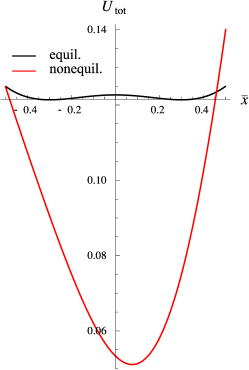
Figure 2: (Color online) Total potential as defined in Eq. (36) for the equilibrium and nonequilibrium system.

In Fig. 2 we display the total potential as defined in Eq. (36). In equilibrium $U_{\rm tot}(\bar{x})$ exhibits a shallow double minimum. The position of the minima corresponds to a stable nuclear coordinate. The minima are symmetric around $\bar{x}=0$ consistently with the symmetry under reflection of the Hamiltonian. In the presence of a bias this reflection symmetry breaks and the current carrying system has only one stable coordinate $\bar{x}_{ss}\simeq 0.088$. The nonequilibrium minimum is much deeper than the equilibrium ones and occurs at a positive $\bar{x}_{ss}$. From the zero-force equation $\bar{x}_{ss}=-(\rho_{ss,11}-\rho_{ss,22})$, and we infer that the occupation on molecule 2 is larger than on molecule 1.

Figure 3: (Color online) Friction coefficient as defined in Eq. (37) for the equilibrium and nonequilibrium system. $\gamma^{(+)}$ is in units of $M\Omega$.

Next we calculate the friction coefficient $\gamma^{(+)}$. The results are displayed in Fig. 3. As expected, in equilibrium the friction is positive for all values of $\bar{x}$. Instead the nonequilibrium friction turns negative in a narrow window of positive $\bar{x}$ values. Interestingly, the steady-state coordinate $\bar{x}_{ss}$ belongs to this window. This means that if we perform AED simulations there is no guarantee that a steady-state is reached. For the model that we are considering the AED equations reduce to

$$\frac{d^{2}\bar{x}}{d\bar{t}^{2}}=-\frac{\partial U_{\rm tot}(\bar{x})}{\partial\bar{x}}-\gamma^{(+)}(\bar{x})\frac{d\bar{x}}{d\bar{t}}$$ (43)

where $\bar{t}=\Omega t$. This equation has the same structure as that of a van der Pol oscillator $\ddot{y}=-y-\gamma(y^{2}-1)\dot{y}$ for which the function multiplying $\dot{y}$ is negative (negative friction) when $y$ is in the range $(-1,1)$ where the stable solution $y=0$ lies. As a consequence of this fact one finds a limit cycle in the momentum-coordinate phase space. In Fig. 4 we show the solution of Eq. (43) in the $\bar{p}-\bar{x}$ plane (with $\bar{p}=d\bar{x}/d{\bar{t}}$) for a situation in which the system has initially a nuclear coordinate $\bar{x}(0)=0.5$ and evolves without any bias or gate voltage (top panel), and for a situation in which the system has initially a nuclear coordinate $\bar{x}(0)=0.04$ and evolves in the presence of a bias $V_{\rm L}=-V_{\rm R}=1$ and gate voltage $v_{\rm C}=0.2$ (bottom panel). For comparison we also illustrate the periodic trajectories corresponding to the solution of Eq. (43) with $\gamma^{(+)}=0$. The main difference between the two panels is that in the current carrying system the nuclear oscillations are not damped. Due to negative friction the trajectory expands outward until reaching a limit cycle. We have checked numerically (not shown) that starting from different $\bar{x}$ the trajectory always tend to the same limit cycle.

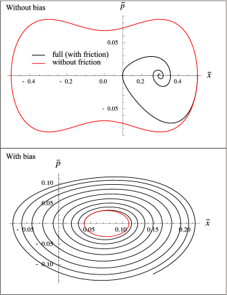
Figure 4: (Color online) Solution of Eq. (43) in the $\bar{p}-\bar{x}$ plane. Top panel. The system evolves without bias starting from an initial nuclear coordinate $\bar{x}(0)=0.5$. Without friction we observe a periodic trajectory which explores both minima of the potential $U_{\rm tot}$, see Fig. 2. In the presence of friction (always positive in this case) the nuclear oscillations are damped and $\bar{x}$ approaches the positive minimum of $U_{\rm tot}$. Bottom panel. The system evolves with a bias $V_{\rm L}=-V_{\rm R}=1$ and gate voltage $v_{\rm C}=0.2$ starting from an initial nuclear coordinate $\bar{x}(0)=0.04$. Without friction we observe a periodic trajectory. Instead with friction the trajectory expand outward until reaching a limit cycle. This is a consequence of the negative friction, see Fig. 3.

III.2 Ehrenfest dynamics simulations

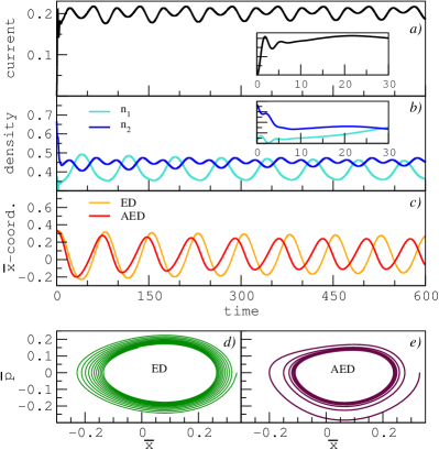
Figure 5: (Color online) Results for a sudden switch-on of the external bias and gate voltage. Time-dependent current flowing between atoms 1 and 2 (panel a) and occupations of atoms 1 and 2 (panel b). A magnification of the initial transient is shown in the insets. Comparison between the ED and AED simulations for the nuclear coordinate (panel c). Trajectories in phase space for the ED (panel d) and AED (panel e) simulations.

We now perform full ED simulations and, instead of studying the evolution of the system when the initial coordinate is arbitrarily chosen by us, we take the system initially in equilibrium and then drive it away from equilibrium using external time-dependent biases and/or gate voltages. In Fig. 5 we suddenly switch on a bias $V_{\rm L}=V_{\rm R}=1$ and a gate voltage $v_{\rm C}=0.2$. These are the same parameters as in the previous Section. Panels a) and b) show the time-dependent current between atoms 1 and 2 and the atomic occupations respectively. After a fast transient (see insets) during which the electrons are not relaxed, these quantities start to oscillate on a nuclear time scale. Despite the DC bias, no steady-state is reached. In panel c) we compare the ED with the AED for the $x$ coordinate. In both cases we observe persistent oscillations of similar amplitude. However the period of these oscillations is different and the curves go out of phase after a few periods. Also the shape of the oscillations is slightly different. In panels d) and e) we put side by side the ED and AED trajectories in phase space. AED reaches the limit cycle much faster than the ED. Apart from these quantitative differences the AED remains a good approximation since during the electronic transient the $x$ coordinate moves very little. Thus at times $t\sim 20/\Omega$ the electrons are essentially relaxed in the initial $x$-coordinate.

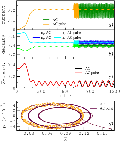
Figure 6: (Color online) Results for a smooth switch-on of the DC bias and gate voltage followed by the switch-on of a superimposed AC bias. Time-dependent current flowing between atoms 1 and 2 (panel a), occupations of atoms 1 and 2 (panel b) and nuclear coordinate (panel c). The curves “AC pulse” refer to simulations in which the AC bias is switched off after $t=700+2\pi\times 10$ (time is in units of $\Omega^{-1}$). Trajectories in phase space (panel d).

New physical scenarios may emerge if the electrons are kept away from their relaxed state. In this context, a central question is: Do the van der Pol oscillations disappear or get distorted? To address the issue, we consider two different time-dependent protocols. As first protocol, we superimpose to the original DC bias a high frequency AC component. In order to isolate the effects of the ultrafast AC component, we switch on the DC bias smoothly. The explicit form of $V_{\rm L}(t)=-V_{\rm R}(t)=V(t)$ is (time is in units of $\Omega^{-1}$)

$$V(t)=\left\{\begin{array}[]{ll}V\sin^{2}(\frac{\pi t}{2\times 250})&\quad t<250\\ V&\quad 250<t<700\\ V+V_{\rm AC}\sin(\omega t)&\quad t>700\end{array}\right.$$ (44)

whereas for the gate voltage $v_{\rm C}(t)=v_{\rm C}\sin^{2}(\frac{\pi t}{2\times 250})$ for $t<250$ and $v_{\rm C}(t)=v_{\rm C}=0.2$ for $t>250$. We maintain the DC component $V=1$ and consider the amplitude $V_{\rm AC}=0.5$ and the frequency $\omega=1$. The time-dependent current (panel a), occupations (panel b) and nuclear coordinate (panel c) are shown in Fig. 6. In this figure we also show results (curve “AC pulse”) of simulations in which the superimposed AC bias is switched off after a time $t=700+2\pi\times 10$. Remarkably the van der Pol oscillations persist in this highly nonadiabatic regime. A glance to the nuclear coordinate (panel c) would suggest that the AC bias is only responsible for increasing the amplitude of the oscillations. This is, however, not the case. The trajectory in phase space (panel d) reveals that the nuclear coordinate feels the nonadiabatic electron dynamics. In fact, we observe cycles with superimposed oscillations of the same frequency $\omega$ as the AC bias. Interestingly an AC pulse can be used to manipulate the radius of the cycles. In the “AC pulse” curve of panel d) the inner cycle sets in before the pulse while the outer cycle sets in after the pulse. The ED is nonperturbative in the velocities and their derivatives, and we are not aware of any mathematical results on the uniqueness of the limit cycle. We therefore addressed this issue numerically. A close inspection to panel d) shows that the inner cycle is moving outward whereas the outer cycle is moving inward, thus suggesting the uniqueness of the limit cycle even within the ED. We performed several simulations with different switching-on protocols of the DC bias and found that cycles with radius larger (smaller) than a critical radius move inward (outward). On the basis of this numerical evidence we conclude that there exists only one limit cycle within the ED. In contrast with the ADE, however, the time to attain the limit cycle is considerably longer; hence cycles of different radius can, de facto, be considered as quasi-stable limit cycles for practical purposes.

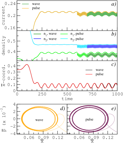
Figure 7: (Color online) Results for a smooth switch-on of the DC bias and gate voltage followed by the switch-on of a superimposed time-dependent gate. Time-dependent current flowing between atoms 1 and 2 (panel a), occupations of atoms 1 and 2 (panel b) and nuclear coordinate (panel c). The curves “wave” and “pulse” refer to simulations in which the time-dependent gate is never switched off and is switched off after $t=695$ (time is in units of $\Omega^{-1}$). Trajectories in phase space for the “wave” (panel d) and “pulse” (panel e) gate.

Similar conclusions are reached when the system is perturbed with a second protocol for a time-dependent perturbation, namely a ultrafast gate voltage. In Fig. 7 we study the response of the system to a train of square pulses in the molecular junction. After the same smooth switching-on of the DC bias and gate as in Fig. 6, we superimpose to $v_{\rm C}=0.2$ the time-dependent gate voltage

$$\delta v_{\rm C}(t)=v_{0}\sum_{n=1}^{\infty}S(t-t_{n})$$ (45)

where $t_{n}=600+n\Delta$ and $S(t)=1$ if $|t|<\Delta/4$ and zero otherwise (time is in units of $\Omega^{-1}$). The calculations are performed with $\Delta=10$ and $v_{0}=0.1$. In the figure the “wave” curves refer to simulations in which $\delta v_{\rm C}(t)$ is never switched off while the “pulse” curves refer to simulations in which $\delta v_{\rm C}(t)$ is switched off after a time $t=695$. The van der Pol oscillations are stable in both cases. An interesting common feature of Figs. 6 and 7 is that the radius of the quasi-stable limit cycle can be tuned by switching off the time-dependent fields at different times. However, if we also want to tune the center of the cycle then the time-dependent fields have to remain on. Both the “AC pulse” curve of Fig. 6 (panel d) and the “pulse” curve of Fig. 7 (panel e) exhibit two concentric cycles. Overall, these features suggest that much more complex nuclear trajectories are to be expected when the electron dynamics in a junction is nonadiabatic.

IV Conclusions and outlook

We have studied the robustness of nuclear van der Pol oscillations in molecular transport when the junction is subject to ultrafast driving fields. In this ultrafast regime the electrons have no time to relax and the adiabatic Ehrenfest dynamics (AED) is no longer justified. We therefore implemented the full Ehrenfest dynamics (ED) using a wavefunction approach. The numerical scheme can deal with arbitrary time-dependent perturbations at the same computational cost and is not limited to wide band leads. We found that the van der Pol oscillations are extremely stable. In the DC case the AED results are in good qualitative agreement with the full ED simulations, as expected. However the ED period of the oscillations as well as the damping time to attain the limit cycle are both longer than those obtained within the AED. In the presence of ultrafast fields the van der Pol oscillations are distorted by the nonadiabatic electron dynamics. In all cases we observed superimposed oscillations of the same frequency as the driving field. We showed that high-frequency biases or gate voltages can be used to tune the amplitude of the oscillations and to shift the average value of the nuclear coordinate. By switching the field off the amplitude remains large for very long times while the average nuclear coordinate goes back to its original value rather fast. Thus, ultra-fast fields can be used to set in quasi-stable limit cycles of desired amplitude. Our numerical evidence suggests that every quasi-stable limit cycle eventually attain a unique limit cycle. We are not aware of any rigorous mathematical proof of this fact.

In this first work we focused on one aspect of current-induced forces, namely the negative friction. In order to observe the nonconservative nature of the steady-state force or the Lorentz-like force one has to consider at least two vibrational modes. The research on current-induced forces is still in its infancy and interesting applications like nanomotors have started to appear in the literature.dmt.2009 ; baj.2008 ; qz.2009 ; brvo.2013 Our results here show that ultrafast fields constitute another knob to tweak nanomechanical engines and that the theoretical scheme we proposed offers a tool to carry on investigations along these lines.

Appendix A Details on the numerical implementation

We consider an arbitrary central region of dimension $M$ described by the one-particle matrix $h$. We choose a basis set $\{|\phi_{i}\rangle,\;i=1,\ldots,M\}$ such that an electron can hop to the left only through the state $|\phi_{1}\rangle$ and to the right only through the state $|\phi_{M}\rangle$. (Here and in the following we use the Greek letter $\phi$ for states strictly localized in region L/R or C and $\psi$ for states of the entire system S=L+C+R.) Let $T_{\rm L}$, $T_{\rm R}$ be the corresponding hopping parameters (in our model system $T_{\rm L}=T_{\rm R}=T_{\rm T}$). The electrodes are described by semi-infinite one-dimensional tight-binding models with nearest neighbor hopping parameter $T_{\rm lead}=T$ (the same for left and right). The one-particle eigenstates of system S can be classified according to their energies. The isolated left and right electrodes have a continuous energy spectrum between $-2|T|$ and $2|T|$. Therefore, one-particle eigenstates with energy $\epsilon<-2|T|$ are bound states with exponential tails in L and R. On the other hand, one-particle eigenstates with energy $\epsilon$ in the band $(-2|T|,2|T|)$ are extended states delocalized all over the system.

Below we compute the degenerate extended states $\psi_{q}^{(a)}$, $a=1,2$, and bound states $\psi_{b}$ in C. We also describe a damped ground state dynamic for the self-consistent solution of Eqs. (10,11). Finally we present an efficient algorithm for the time-propagation.

A.1 Extended states

Delocalized states are twice degenerate and we denote by $\psi_{q}^{(1)}$ and $\psi_{q}^{(2)}$ the two eigenfunctions with eigenenergy $\epsilon_{q}=2T\cos\left(q\right)$, $q\in(0,\pi)$. The eigenvalue equation in region C reads

$$\sum_{j=1}^{M}\left(\epsilon_{q}\delta_{ij}-h_{ij}\right)\psi_{q}^{(a)}(j)=\delta_{i,1}T_{\rm L}\psi_{q}^{(a)}(\rm L)\;$$

$$+\delta_{i,M}T_{\rm R}\psi_{q}^{(a)}(\rm R),$$ (46)

where $\psi_{q}^{(a)}(\alpha)$, $\alpha={\rm L,R}$, is the amplitude of the wave function on the first site of electrode $\alpha$ and $\psi_{q}^{(a)}(j)\equiv\langle\phi_{j}|\psi_{q}^{(a)}\rangle$. We diagonalize $h$ and find eigenstates $|\lambda_{\mu}\rangle$ with eigenenergies $\epsilon_{\mu}$ (the index $\mu$ runs between 1 and $M$). In terms of $|\lambda_{\mu}\rangle$ and $\epsilon_{\mu}$ Eq. (46) can be rewritten as

$$\psi_{q}^{(a)}(i) = T_{\rm L}\psi_{q}^{(a)}({\rm L})\sum_{\mu=1}^{M}\frac{\langle\phi_{i}|\lambda_{\mu}\rangle\langle\lambda_{\mu}|\phi_{1}\rangle}{\epsilon_{q}-\epsilon_{\mu}}$$ (47)

$$+ T_{\rm R}\psi_{q}^{(a)}({\rm R})\sum_{\mu=1}^{M}\frac{\langle\phi_{i}|\lambda_{\mu}\rangle\langle\lambda_{\mu}|\phi_{M}\rangle}{\epsilon_{q}-\epsilon_{\mu}},$$

with $i=1,\ldots,M$. This equation allows us to obtain the amplitude of extended states in C provided that $\epsilon_{q}\neq\epsilon_{\mu}$, $\forall\mu$. Indeed, we can exploit the degeneracy of $\epsilon_{q}$ and choose the vectors $\left(\psi_{q}^{(1)}({\rm L}),\psi_{q}^{(1)}({\rm R})\right)$, $\left(\psi_{q}^{(2)}({\rm L}),\psi_{q}^{(2)}({\rm R})\right)$ as we please. Of course, in order to obtain two independent eigenvectors $\psi_{q}^{(1)}(\alpha)\neq C\psi_{q}^{(2)}(\alpha)$, $\alpha={\rm L,R}$, with $C$ complex number.

Having the projection of $|\psi_{q}^{(a)}\rangle$ onto region C we can match it to the analytic form in the leads. We first use the Schrödinger equation to calculate $\psi_{q}^{(a)}(k)$ on sites $k={\rm L}+1,{\rm L}+2$ (second and third sites of electrode L) and $k={\rm R}+1,{\rm R}+2$ (second and third sites of electrode R). Then we use $\psi_{q}^{(a)}(k)$ to compute the phase shift and the amplitudes of the oscillation in $\alpha={\rm L,R}$

$$\psi_{q}^{(a)}(\alpha+m)=A_{q,\alpha}^{(a)}\sin\left(qm+\delta_{q,\alpha}^{(a)}\right),\quad m=1,2.$$ (48)

The two degenerate eigenfunctions $\psi_{q}^{(1)}$ and $\psi_{q}^{(2)}$ are independent by construction but not orthonormal. In order to orthonormalize them we need the overlap $N_{aa^{\prime}}=2\langle\psi_{q}^{(a)}|\psi_{q}^{(a^{\prime})}\rangle/(\pi\delta(0))$. It is straightforward to show that

$$N_{aa^{\prime}} = A_{q,\rm L}^{(a)}A_{q,\rm L}^{(a^{\prime})}\cos\left(\delta^{(a)}_{q,\rm L}-\delta_{q,\rm L}^{(a^{\prime})}\right)$$ (49)

$$+ A_{q,\rm R}^{(a)}A_{q,\rm R}^{(a^{\prime})}\cos\left(\delta^{(a)}_{q,\rm R}-\delta_{q,\rm R}^{(a^{\prime})}\right).$$

The wave functions $\psi_{q}^{(a)}$ are eventually normalized according to $\langle\psi_{q}^{(a)}|\psi_{q^{\prime}}^{(a^{\prime})}\rangle=2\pi\delta_{aa^{\prime}}\delta(q-q^{\prime})$.

A.2 Bound states

Without loss of generality we choose the hopping parameter $T<0$ in the left and right electrodes. Let $|\psi_{b}\rangle$ be a possible bound state of energy $\epsilon_{b}<-2|T|$. As for the extended states, the wavefunction in region C is completely determined by the amplitudes $\psi_{b}(\alpha)$, $\alpha={\rm L,R}$ on the first site of electrode $\alpha$, see Eq. (46). The amplitudes $\psi_{b}(\rm L)$ and $\psi_{b}(\rm R)$ can be expressed in terms of $\psi_{b}(1)=\langle\phi_{1}|\psi_{b}\rangle$ and $\psi_{b}(M)=\langle\phi_{M}|\psi_{b}\rangle$ respectively. We have

$$\psi_{b}({\rm L})=T_{\rm L}\;g(\epsilon_{b})\psi_{b}(1),\quad\psi_{b}({\rm R})=T_{\rm R}\;g(\epsilon_{b})\psi_{b}(M),$$ (50)

where $g(\omega)$ is the retarded Green’s function of a semi-infinite chain. For $\omega<-2|T|$

$$g(\omega)=\frac{\omega+\sqrt{\omega^{2}-4T^{2}}}{2T^{2}}.$$ (51)

Using Eqs. (50), the Schrödinger equation in region C reads

$$\sum_{j=1}^{M}\left(\epsilon_{b}\delta_{ij}-h_{ij}-\Sigma^{\rm R}_{ij}(\epsilon_{b})\right)\psi_{b}(j)=0,$$ (52)

where the embedding self-energy $\Sigma^{\rm R}(\omega)$ is a $M\times M$ matrix having only two non-vanishing matrix elements: the (1,1) element which is equal to $T_{\rm L}^{2}g(\omega)$ and the $(M,M)$ element which is equal to $T_{\rm R}^{2}g(\omega)$. Bound-state energies $\epsilon_{b}$ are given by the solutions of

$$D(\omega)\equiv{\rm Det}\left[\omega-h-\Sigma^{\rm R}(\omega)\right]=0,$$ (53)

with $\omega<-2|V|$. The corresponding bound state in C can be calculated from Eq. (52).

In analogy with the procedure described in Section A.1 we extended the bound-state wave function up to the second and third sites of electrode $\alpha={\rm L,R}$, matched it to the analytic form in the leads

$$\psi_{b}(\alpha+m)=A_{b,\alpha}e^{-\lambda_{b,\alpha}m},\quad m=1,2,$$ (54)

and calculated the amplitudes $A_{b,\alpha}$ and penetration lengths $\lambda_{b,\alpha}$. Knowing $|\psi_{b}\rangle$ in region C and in the leads we can calculate

$$\langle\psi_{b}|\psi_{b}\rangle=\sum_{j=1}^{M}|\psi_{b}(j)|^{2}+\sum_{\alpha=\rm L,R}\frac{A_{b,\alpha}^{2}}{1-e^{-2\lambda_{b,\alpha}}}$$ (55)

and normalize the bound-state wavefunction.

A.3 Ground state

The parametric dependence of $\hat{H}_{\rm el}$ on the coordinates ${\bf x}$ renders every eigenstate a function of ${\bf x}$. We use the notation $|\psi_{q}^{(a)}[{\bf x}]\rangle$ and $|\psi_{b}[{\bf x}]\rangle$ for extended and bound states of $\hat{H}_{\rm el}[{\bf x}]$. Let us consider the ground state $|\Psi_{g}\rangle=|\Psi_{g}[{\bf x}]\rangle$ of $\hat{H}_{\rm el}[{\bf x}]$. $|\Psi_{g}[{\bf x}]\rangle$ is a Slater determinant formed by all bound states $|\psi_{b}[{\bf x}]\rangle$ and extended states $|\psi_{q}^{(a)}[{\bf x}]\rangle$ with energy below the chemical potential $\mu=2|T|\cos(q_{\rm F})$. The ground state value ${\bf x}_{g}$ of the nuclear coordinates can be computed from the zero-force equation (10). In our practical implementation we constructed the one-particle density matrix of Eq. (11)

$$\rho_{g,ji}[{\mathbf{x}}] = \sum_{b}\psi_{b}[{\mathbf{x}}]^{\ast}(i)\psi_{b}[{\mathbf{x}}](j)$$ (56)

$$+ \sum_{a=1}^{2}\int_{0}^{q_{\rm F}}\frac{dq}{2\pi}\psi_{q}^{(a)}[{\bf x}]^{\ast}(i)\psi_{q}^{(a)}[{\bf x}](j)$$

and then evolved the coordinates according to the fictitious damped dynamics

$$M_{n}\ddot{x}_{n}=-\gamma\dot{x}_{n}-\frac{\partial U_{\rm cl}({\mathbf{x}})}{\partial x_{n}}-\sum_{ij}\frac{\partial h_{ij}({\mathbf{x}})}{\partial x_{n}}\rho_{g,ji}({\mathbf{x}})$$ (57)

with $\gamma>0$ some friction coefficient. Due to the multivalley nature of the potential, the damped dynamics might not converge to the lowest-energy solution. We therefore embedded C in in finite rings of increasing length $L$, found the energy minimum ${\mathbf{x}}_{g}(L)$ and used its extrapolated value ${\mathbf{x}}_{g}(L\rightarrow\infty)$ as initial condition for the fictitious dynamics.

This concludes the description of the numerical algorithm used to find the ground state configuration of $\hat{H}_{\rm el}[{\bf x}]+H_{\rm cl}[{\bf p},{\bf x}]$. In the next Section we present how to propagate the electronic wavefunctions and the nuclear coordinates when the system is disturbed by external driving fields.

A.4 Time evolution

The evolution is governed by Eqs. (6,7,8). It is convenient to rearrange the electronic Hamiltonian matrix $h_{\rm el}$ of the entire system S=L+C+R as

$$h_{\rm el}({\bf x}(t),t)=h_{0}({\bf x}(t),t)+v(t)$$ (58)

where $h_{0}$ depends on time only through the central region

$$h_{0}({\bf x}(t),t)=\left(\begin{array}[]{ccc}h_{\rm L}&h_{\rm LC}&0\\ h_{\rm CL}&h({\bf x}(t),t)&h_{\rm CR}\\ 0&h_{\rm RC}&h_{\rm R}^{0}\end{array}\right),$$ (59)

whereas

$$v(t)=\left[\begin{array}[]{ccc}V_{\rm L}(t)&0&0\\ 0&0&0\\ 0&0&V_{\rm R}(t)\end{array}\right]$$ (60)

describes the perturbation due to the bias.

For the time-propagation we discretize the time $t_{m}=2m\delta$ (where $\delta$ is an infinitesimal quantity and $m$ is an integer). We first propagate all occupied wavefunctions from $t_{m}$ to $t_{m+1}$ using the algorithm of Ref. ksarg.2005, . Then we propagate coordinates and momenta from $t_{m}$ to $t_{m+2}$ using a Verlet-like algorithm. Finally, we complete the propagation of a full time step $\Delta=4\delta$ by evolving the wavefunctions from $t_{m+1}$ to $t_{m+2}$. The overall scheme for the time-propagation reads

$$(1+i\delta h_{0}^{(m)})\frac{1+i\frac{\delta}{2}v^{(m)}}{1-i\frac{\delta}{2}v^{(m)}}|\psi_{s}^{(m+1)}\rangle=(1-i\delta h_{0}^{(m)})\frac{1-i\frac{\delta}{2}v^{(m)}}{1+i\frac{\delta}{2}v^{(m)}}|\psi_{s}^{(m)}\rangle,\quad\forall\psi_{s}\in{\rm occ}$$ (61)

$$\left\{\begin{array}[]{l}p_{n}^{(m+1)}=p_{n}^{(m)}+2\delta F_{n}[{\bf x}^{(m)},\{\psi_{s}^{(m+1)}\}]\\ x_{n}^{(m+2)}=x_{n}^{(m)}+4\delta p_{n}^{(m+1)}/M_{n}\\ p_{n}^{(m+2)}=p_{n}^{(m+1)}+2\delta F_{n}[{\bf x}^{(m+2)},\{\psi_{s}^{(m+1)}\}]\end{array}\right.$$ (62)

$$(1+i\delta h_{0}^{(m+2)})\frac{1+i\frac{\delta}{2}v^{(m+1)}}{1-i\frac{\delta}{2}v^{(m+1)}}|\psi_{s}^{(m+2)}\rangle=(1-i\delta h_{0}^{(m+2)})\frac{1-i\frac{\delta}{2}v^{(m+1)}}{1+i\frac{\delta}{2}v^{(m+1)}}|\psi_{s}^{(m+1)}\rangle,\quad\forall\psi_{s}\in{\rm occ}$$ (63)

with $m=0,2,4,6,\ldots$. In these equations $h_{0}^{(m)}=h_{0}({\mathbf{x}}(t_{m}),t_{m})$ and $v^{(m)}=\frac{1}{2}[v(t_{m+1})+v(t_{m})]$. We also used the short-hand notation $\psi_{s}^{(m)}=\psi_{s}(t_{m})$, ${\bf x}^{(m)}={\bf x}(t_{m})$ and ${\bf p}^{(m)}={\bf p}(t_{m})$. The initial values are ${\bf x}^{(0)}={\bf x}_{g}$, ${\bf p}^{(0)}=0$ and $\{\psi_{s}^{(0)}\}=\{\psi_{s}\}$ ($\{\psi_{s}\}$ being the set of occupied one-particle eigenstates). In Eq. (62), the force $F_{n}[{\bf x},\{\psi_{s}\}]$ depends on the coordinates and on the one-particle eigenstates and is given by the right hand side of Eq. (8).

References

- (1) R. E. Peierls, Quantum Theory of Solids (Clarendon, Oxford, 1955).
- (2) See for instance G. D. Mahan, Many-particle Physics, 2nd ed. (Plenum Press, New York, 1990).
- (3) Electron and Phonons, J. M. Ziman (Oxford University Press, 1960).
- (4) E. Dagotto, Rev. Mod. Phys. 66, 763 (1994).
- (5) G. Hunter, Int. J. Quantum Chem. 9, 237 (1975).
- (6) A. Abedi, N. T. Maitra, and E. K. U. Gross, Phys. Rev. Lett. 105, 123002 (2010).
- (7) R. Car, and M. Parrinello, Phys. Rev. Lett. 55, 2471 (1985).
- (8) Electron-Phonon Interactions in Low-Dimensional Structures, L. Challis ed., Oxford U. P., Oxford (2003).
- (9) J. C. Cuevas and E. Scheer, Molecular Electronics An Introduction to Theory and Experiment (World Scientific Publishing Co, Hackensack, 2010)
- (10) A. A. Balandin, J. Nanosci. Nanotechnol. 5, 1015 (2005).
- (11) E. G. Emberly and G. Kirczenow, Phys. Rev. B 64, 125318 (2001).
- (12) T. N. Todorov, J. Hoekstra, and A. P. Sutton, Phys. Rev. Lett. 86, 3606 (2001).
- (13) M. Di Ventra, S. T. Pantedelis and N. D. Lang, Phys. Rev. Lett. 88, 046801 (2002).
- (14) M. Brandbyge, K. Stokbro, J. Taylor, J. L. Mozos, and P. Ordejon, Phys. Rev. B 67, 193104 (2003).
- (15) M. Cizek, M. Thoss and W. Domcke, Phys. Rev. B 70, 125406 (2004).
- (16) P. S. Cornaglia, H. Ness, and D. R. Grempel, Phys. Rev. Lett. 93, 147201 (2004).
- (17) T. Frederiksen, M. Brandbyge, N. Lorente and A.-P. Jauho, Phys. Rev. Lett. 93, 256601 (2004).
- (18) M. Paulsson, T. Frederiksen, and M. Brandbyge, Phys. Rev. B 72, 201101(R) (2005).
- (19) T. Frederiksen, M. Paulsson, M. Brandbyge and A. P. Jauho, Phys. Rev. B 75 205413 (2007).
- (20) M. Galperin, A. Nitzan and M. A Ratner, J. Phys. Condens. Matter 19, 103201 (2007).
- (21) M. Galperin, A. Nitzan and M. A Ratner, J. Phys. Condens. Matter 20, 374107 (2008).
- (22) R. Härtle, C. Benesch, and M. Thoss, Phys. Rev. Lett. 102, 146801 (2009).
- (23) R. Zhang, I. Rungger, S. Sanvito and S. Hou, Phys. Rev. B 84, 085445 (2011).
- (24) K. F. Albrecht, H. Wang, L. Mühlbacher, M. Thoss and A. Komnik, Phys. Rev. B 86, 081412 (2012).
- (25) A. P. Horsfield, D. R. Bowler, and A. J. Fisher, J. Phys. Condens. Matter 16, L65 (2004).
- (26) A. P. Horsfield, D. R. Bowler, A. J. Fisher, T. N. Todorov and C. G. Sánchez, J. Phys. Condens. Matter 16, 8251 (2004).
- (27) C. Verdozzi, G. Stefanucci and C. O. Almbladh, Phys. Rev. Lett. 97, 046603 (2006).
- (28) C. Sanchez, M. Stamenova, S. Sanvito, D.R. Bowler, A.P. Horsfield, and T. Todorov, J. Chem. Phys., 124, 214708, (2006).
- (29) M. Todorovic and D. R. Bowler, J. Phys. Condens. Matter 23, 345301 (2011).
- (30) D. Dundas, E. J. McEniry and T. N. Todorov, Nat. Nanotech. 4, 99 (2009).
- (31) T. N. Todorov, D. Dundas and E. J. McEniry, Phys Rev. B 81, 075416 (2010).
- (32) R. Hussein, A. Metelmann, P. Zedler and T. Brandes, Phys. Rev. B 82, 165406 (2010).
- (33) J. T. Lü, P. Hedegard and M. Brandbyge, Phys. Rev. Lett. 107, 046801 (2011).
- (34) J. T. Lü, M. Brandbyge and P. Hedegard, NanoLett. 10, 1657 (2010).
- (35) N. Bode, S. V. Kusminskiy, R. Egger and F. von Oppen, Phys. Rev. Lett. 107, 036804 (2011).
- (36) N. Bode, S. V. Kusminskiy, R. Egger and F. von Oppen, Beilstein J. Nanotechnol. 3, 144 (2012).
- (37) S. D. Bennett and A. A. Clerk, Phys. Rev. B 74, 201301 (2006).
- (38) A. Metelmann and T. Brandes, Phys Rev. B 84, 155455 (2011).
- (39) A. Nocera, C. A. Perroni, V. Marigliano Ramaglia and V. Cataudella, Phys. Rev. B 83, 115420 (2011).
- (40) S. Kurth, G. Stefanucci, C.-O. Almbladh, A. Rubio and E. K. U. Gross, Phys. Rev. B 72, 035308 (2005).
- (41) G. Stefanucci and R. van Leeuwen, Nonequilibrium Many-Body Theory of Quantum Systems: A Modern Introduction (Cambridge University Press, 2013).
- (42) G. Stefanucci, Phys. Rev. B 75, 195115 (2007).
- (43) S. W. D. Bailey, I. Amanatidis and C. J. Lambert, Phys. Rev. Lett. 100, 256802 (2008).
- (44) X. L. Qi and S. C. Zhang, Phys. Rev. B 79, 235442 (2009).
- (45) R. Bustos-Marún, G. Refael and F. von Oppen, arXiv:1304.4969.