Quantized Iterative Hard Thresholding:
Bridging 1-bit and High-Resolution
Quantized Compressed Sensing

Abstract

In this work, we show that reconstructing a sparse signal from quantized compressive measurement can be achieved in an unified formalism whatever the (scalar) quantization resolution, i.e., from 1-bit to high resolution assumption. This is achieved by generalizing the iterative hard thresholding (IHT) algorithm and its binary variant (BIHT) introduced in previous works to enforce the consistency of the reconstructed signal with respect to the quantization model. The performance of this algorithm, simply called quantized IHT (QIHT), is evaluated in comparison with other approaches (e.g., IHT, basis pursuit denoise) for several quantization scenarios.

1 Introduction

Since the advent of Compressed Sensing (CS) almost 10 years ago [1, 2], many works have treated the problem of inserting this theory into an appropriate quantization scheme. This step is indeed mandatory for transmitting, storing and even processing any compressively acquired information, and more generally for sustaining the embedding of the CS principle in sensor design.

In its most popular version, CS provides uniform theoretical guarantees for stably recovering any sparse (or compressible) signal at a sensing rate proportional to the signal intrinsic dimension (i.e., its sparsity level) [1, 2]. In this context, scalar quantization of compressive measurements has been considered along two main directions.

First, under a high-resolution quantization assumption, i.e., when the number of bits allocated to encode each measurement is high, the quantization impact is often modeled as a mere additive Gaussian noise whose variance is adjusted to the quantization $\ell_{2}$-distortion [3]. In short, under this high-rate model, the CS stability guarantees under additive Gaussian noise, i.e., as derived from the $\ell_{2}-\ell_{1}$ instance optimality [2], are used to bound the reconstruction error obtained from quantized observations. Variants of these works handle quantization saturation [4], prequantization noise [5], $\ell_{p}$-distortion models ($p\geq 2$) for improved reconstruction in oversampled regimes [6, 7], optimize the high-resolution quantization procedure [8] or integrate more evolved $\Sigma\Delta$-quantization models departing from scalar PCM quantization [9].

Second, and more recently, extreme 1-bit quantization recording only the sign of the compressive measurement, i.e., an information encoded in a single bit, has been considered [10, 11, 12, 13]. New guarantees have been developed to tackle the non-linear nature of the sign operation thanks to the replacement of the restricted isometric property (RIP) by the quasi-isometric binary $\epsilon$-stable embedding (B$\epsilon$SE) [11], or to more general characterization of the binary embedding of sets based on their Gaussian Mean Width [12, 13]. In this context, iterative methods such as the binary iterative hard thresholding [11] or linear programming optimization [12] have been introduced for estimating the 1-bit sensed signal.

This work proposes a general procedure for handling the reconstruction of sparse signals observed according to a standard non-uniform scalar quantization of the compressive measurements. The novelty of this scheme is its ability to handle any resolution level, from 1-bit to high-resolution, in a progressive fashion. Conversely to the Bayesian approach of [15], our method relies on a generalization of the iterative hard thresholding (IHT) [16] that we simply called quantized iterative hard thresholding. Actually, QIHT reduces to BIHT for 1-bit sensing and it converges to IHT at high resolution.

Conventions

Most of domain dimensions (e.g., $M$, $N$) are denoted by capital roman letters. Vectors and matrices are associated to bold symbols while lowercase light letters are associated to scalar values. The $i^{\rm th}$ component of a vector $\bm{u}$ is $u_{i}$ or $(\bm{u})_{i}$. The identity matrix is $\operatorname{\bf Id}$. The set of indices in $\mathbb{R}^{D}$ is $[D]=\{1,\,\cdots,D\}$. Scalar product between two vectors $\bm{u},\bm{v}\in\mathbb{R}^{D}$ reads $\bm{u}^{*}\bm{v}=\langle\bm{u},\bm{v}\rangle$ (using the transposition $(\cdot)^{*}$), while the Hadamard product $\bm{u}\odot\bm{v}$ is such that $(\bm{u}\odot\bm{v})_{i}=u_{i}v_{i}$. For any $p\geq 1$, $\|\cdot\|_{p}$ represents the $\ell_{p}$-norm such that $\|\bm{u}\|_{p}^{p}=\sum_{i}|u_{i}|^{p}$ with $\|\bm{u}\|=\|\bm{u}\|_{2}$ and $\|\bm{u}\|_{\infty}=\max_{i}|u_{i}|$. The $\ell_{0}$ “norm” is $\|\bm{u}\|_{0}=\#{\rm supp}\,\bm{u}$, where $\#$ is the cardinality operator and ${\rm supp}\,\bm{u}=\{i:u_{i}\neq 0\}\subseteq[D]$. For $\mathcal{S}\subseteq[D]$, $\bm{u}_{\mathcal{S}}\in\mathbb{R}^{\#\mathcal{S}}$ (or $\bm{\Phi}_{\mathcal{S}}$) denotes the vector (resp. the matrix) obtained by retaining the components (resp. columns) of $\bm{u}\in\mathbb{R}^{D}$ (resp. $\bm{\Phi}\in\mathbb{R}^{D^{\prime}\times D}$) belonging to $\mathcal{S}\subseteq[D]$. The operator $\mathcal{H}_{K}$ is the hard thresholding operator setting all the coefficients of a vector to 0 but those having the $K$ strongest amplitudes. The set of canonical $K$-sparse vectors in $\mathbb{R}^{N}$ is $\Sigma_{K}=\{\bm{v}\in\mathbb{R}^{N}:\|\bm{v}\|_{0}\leq K\}$ while $\Sigma_{\mathcal{T}}$ denotes the set of vectors whose support is $\mathcal{T}\subseteq[N]$. Moreover, $\Sigma^{*}_{K}=\Sigma_{K}\cap S^{N-1}$ and $\Sigma^{*}_{\mathcal{T}}=\Sigma^{*}_{\mathcal{T}}\cap S^{N-1}$ with $S^{N-1}$ the $(N-1)$-sphere in $\mathbb{R}^{N}$. Finally, $\chi_{\mathcal{I}}$ is the characteristic function on $\mathcal{I}\subset\mathbb{R}$, ${\rm sign}\,\lambda$ equals $1$ if $\lambda$ is positive and $-1$ otherwise, $(\lambda)_{+}=(\lambda+|\lambda|)/2$ and $(\lambda)_{-}=-(-\lambda)_{+}$ project $\lambda$ on $\mathbb{R}_{+}$ and $\mathbb{R}_{-}$, respectively, with all these operators being applied component wise onto vectors.

2 Noisy Compressed Sensing Framework

The iterative hard thresholding (IHT) algorithm has been introduced for iteratively reconstructing a sparse or compressible signal $\bm{x}\in\mathbb{R}^{N}$ from compressible observations $\bm{y}=\bm{\Phi}\bm{x}+\bm{n}$, where $\bm{\Phi}\in\mathbb{R}^{M\times N}$ is the sensing matrix and $\bm{n}\in\mathbb{R}^{M}$ stands for a possible observational noise with bounded energy $\|\bm{n}\|\leq\varepsilon$. IHT is an alternative to the basis pursuit denoise (BPDN) method [17] which aims at solving a global convex minimization promoting a $\ell_{1}$-sparse data prior model under the constraint of reproducing the compressive observation.

Assuming that $\bm{x}$ is $K$-sparse in the canonical basis $\bm{\Psi}=\operatorname{\bf Id}$, i.e., $\bm{x}\in\Sigma_{K}$, the IHT algorithm is designed to approximately solve the (LASSO-type) problem

$$\min_{\bm{u}\in\mathbb{R}^{N}}{\textstyle\frac{1}{2}}\|\bm{y}-\bm{\Phi}\bm{u}\|^{2}\ \text{s.t.}\ \|\bm{u}\|_{0}\leq K.\vspace{0mm}$$ (1)

It proceeds by computing the following recursion

$$\bm{x}^{(n+1)}=\mathcal{H}_{K}\big{[}\bm{x}^{(n)}+\mu\bm{\Phi}^{*}(\bm{y}-\bm{\Phi}\bm{x}^{(n)})\big{]},\vspace{0mm}$$ (IHT)

where $\bm{x}^{(0)}=\bm{0}$, and $\mu>0$ must satisfy $\mu^{-2}>\|\bm{\Phi}\|:=\sup_{\bm{u}:\|\bm{u}\|=1}\|\bm{\Phi}\bm{u}\|$ for guaranteeing convergence [18].

In other words, at each iteration, starting from the previous estimation $\bm{x}^{(n)}$, the fidelity function $\mathcal{E}(\bm{u}):={\textstyle\frac{1}{2}}\|\bm{y}-\bm{\Phi}\bm{u}\|^{2}$ is decreased by a gradient descent step with gradient $\bm{\nabla}\mathcal{E}(\bm{x}^{(n)})=\bm{\Phi}^{*}(\bm{\Phi}\bm{x}^{(n)}-\bm{y})$, followed by a “projection” on $\Sigma_{K}$ accomplished by the hard thresholding $\mathcal{H}_{K}$.

In [16], it is shown that if $\bm{\Phi}$ respects the restricted isometry property (RIP) of order $3K$ with radius $\delta_{3K}<1/15$, which means that for all $\bm{u}\in\Sigma_{3K}$, $(1-\delta_{3K})\|\bm{u}\|^{2}\leq\|\bm{\Phi}\bm{u}\|^{2}\leq(1+\delta_{3K})\|\bm{u}\|^{2}$, then, at iteration $n^{*}=\lceil\log_{2}\|\bm{x}\|/\varepsilon\rceil$, the reconstruction error satisfies $\|\bm{x}-\bm{x}^{(n^{*})}\|\leq 5\varepsilon$.

3 Quantized Sensing Model

For the sake of simplicity, let us consider a unit $K$-sparse signal $\bm{x}_{0}\in\Sigma^{*}_{K}$ observed through the following Quantized Compressed Sensing (QCS) model

$$\bm{y}=\mathcal{Q}_{b}[\bm{\Phi}\bm{x}_{0}],\vspace{0mm}$$ (2)

where $\bm{\Phi}\in\mathbb{R}^{M\times N}$ is the sensing matrix and $\mathcal{Q}_{b}$ the quantization operator defined at a resolution of $b$-bits per measurement, i.e., with no further encoding treatment, $\bm{y}$ requires a total of $\mathfrak{B}=bM$ bits. In this work, we will not consider any prequantization noise in (2).

The quantization $\mathcal{Q}_{b}$ is assumed optimal with respect to the distribution of each component of $\bm{z}=\bm{\Phi}\bm{x}_{0}\in\mathbb{R}^{M}$. In particular, by considering only random Gaussian matrices $\bm{\Phi}\sim\mathcal{N}^{M\times N}(0,1)$, i.e., where each matrix entry follows $\Phi_{ij}\sim_{\rm iid}\mathcal{N}(0,1)$, we have $z_{i}\sim\mathcal{N}(0,\|\bm{x}_{0}\|^{2}=1)$ and we adjust $\mathcal{Q}_{b}$ to an optimal $b$-bits Gaussian Quantizer minimizing the quantization distortion, e.g., using a Lloyd-Max optimization [19]. This provides a set of thresholds $\{\tau_{i}\in\bar{\mathbb{R}}:1\leq i\leq 2^{b}+1\}$ (with $-\tau_{1}=\tau_{2^{b}+1}=+\infty$) defining $2^{b}$ quantization bins $\mathcal{R}_{i}=[\tau_{i},\tau_{i+1})$, and a set of levels $\{q_{i}\in\mathcal{R}_{i}:1\leq i\leq 2^{b}\}$ such that

$$\mathcal{Q}_{b}[\lambda]=q_{k}\ \Leftrightarrow\ \lambda\in\mathcal{R}_{k},\vspace{0mm}$$

with $2\tau_{i}=q_{i-1}+q_{i}$ and $q_{i}=\mathbb{E}[g_{x}|g_{x}\in\mathcal{R}_{i}]$ with $g_{x}\sim\mathcal{N}(0,1)$. Notice that this QCS model includes 1-bit CS scheme since $\mathcal{Q}_{1}[\lambda]=q_{0}\,{\rm sign}\,(\lambda)$ with $q_{0}:=q_{2}=-q_{1}=\sqrt{2/\pi}$.

4 Quantized Iterative Hard Thresholding

In this section, we propose a generalization of the IHT algorithm taking into account the particular nature of the scalar quantization model introduced in Sec. 3. The idea is to enforce the consistency of the iterates with the quantized observations. This is first achieved by defining an appropriate cost measuring deviation from quantization consistency.

Given $\nu,\lambda\in\mathbb{R}$ and using the levels and thresholds associated to $\mathcal{Q}_{b}$, we first define

$$J(\nu,\lambda) =\sum_{j=2}^{2^{b}}w_{j}\,\big{|}\big{(}{\rm sign}\,(\lambda-\tau_{j})\,(\nu-\tau_{j})\big{)}_{-}\big{|},\vspace{0mm}\vspace{0mm}$$ (3)

with $w_{j}=q_{j}-q_{j-1}$. Equivalently, given $\mathcal{I}(\nu,\lambda):=[\min(\nu,\lambda),\max(\nu,\lambda)]$, $J(\nu,\lambda)=\sum_{j=2}^{2^{b}}w_{j}\chi_{\mathcal{I}}(\tau_{j})\,|\nu-\tau_{j}|$. The non-zero terms are therefore determined by the thresholds lying between $\lambda$ and $\nu$, i.e., for which ${\rm sign}\,(\lambda-\tau_{j})\neq{\rm sign}\,(\nu-\tau_{j})$. Interestingly, $J(\nu;\lambda)=J(\nu;\mathcal{Q}_{b}(\lambda))$ since ${\rm sign}\,(\lambda-\tau_{j})={\rm sign}\,(\mathcal{Q}_{b}(\lambda)-\tau_{j})$ for all $j\in[2^{b}+1]$.

Then, our quantization consistency function between two vectors $\bm{u},\bm{v}\in\mathbb{R}^{M}$ reads

$$\mathcal{J}(\bm{u},\bm{v}):=\sum_{k=1}^{M}J(u_{k},v_{k})=\mathcal{J}(\bm{u},\mathcal{Q}_{b}(\bm{v})).\vspace{0mm}$$ (4)

This cost, which is convex with respect to $\bm{u}$, has two interesting limit cases. First, for $b=1$, it reduces to the cost on which relies the binary iterative hard thresholding algorithm (BIHT) adapted to 1-bit CS [11]. In this context, the sum in (3) has only one term (for $j=2$) and $\mathcal{J}(\bm{u},\bm{v})=2q_{0}\,\|({\rm sign}\,(\bm{v})\odot\bm{u})_{-}\|_{1}$. Up to a normalization by $2q_{0}$, this is the $\ell_{1}$-sided norm minimized by BIHT which vanishes when $q_{0}\,{\rm sign}\,(\bm{u})=\mathcal{Q}_{1}(\bm{u})=\mathcal{Q}_{1}(\bm{v})=q_{0}\,{\rm sign}\,(\bm{v})$, with $q_{0}$ defined in Sec. 3.

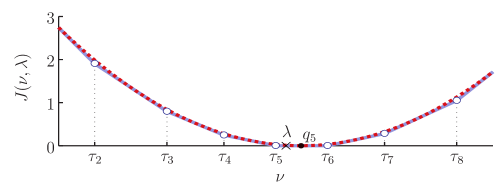
Figure 1: (plain curve) Plot of $J$ as a function of $\nu\in\mathbb{R}$ for $b=3$ ($\tau_{5}=0$) and $\lambda\in\mathcal{R}_{5}$. (dashed curve) Plot of ${\textstyle\frac{1}{2}}(\nu-q_{5})^{2}$.

Second, in the high resolution limit when $b\gg 1$, $\mathcal{J}(\bm{u},\bm{v})$ tends to ${\textstyle\frac{1}{2}}\|\bm{u}-\bm{v}\|^{2}$. Indeed, in this case $w_{j}\ll 1$ and, the sum in (3) tends to

$$J(\nu,\lambda)\simeq\big{|}{\textstyle\int}_{\nu}^{\lambda}(\nu-t)\,\mathrm{d}t\,\big{|}={\textstyle\frac{1}{2}}(\nu-\lambda)^{2}.$$

This asymptotic quadratic behavior of $J$ is illustrated in Fig. 1.

Given the quantization consistency cost $\mathcal{J}$, we can now formulate a generalization of (1) for estimating a $K$-sparse signal $\bm{x}_{0}$ observed by the model (2):

$$\min_{\bm{u}\in\mathbb{R}^{N}}\mathcal{E}_{b}(\bm{u})\ \text{s.t.}\ \|\bm{u}\|_{0}\leq K,$$ (5)

with $\mathcal{E}_{b}(\bm{u}):=\mathcal{J}(\bm{\Phi}\bm{u},\bm{y})=\mathcal{J}(\bm{\Phi}\bm{u},\mathcal{Q}_{b}[\bm{\Phi}\bm{x}_{0}])$.

Following the procedure determining the IHT algorithm from (1) (Sec. 2), our aim is to find an IHT variant which minimizes the quantization inconsistency, as measured by $\mathcal{E}_{b}$, instead of the quadratic cost $\mathcal{E}$. This is done by first determining a subgradient of the convex but non-smooth function $\mathcal{E}_{b}$ [20].

A quick calculation shows that a subdifferential of $J(\nu,\lambda)$ with respect to $\nu$ reads

$$\sum_{j=k_{-}+1}^{k_{+}}\tfrac{w_{j}}{2}({\rm sign}\,(\nu-\tau_{j})-{\rm sign}\,(\lambda-\tau_{j})),\vspace{0mm}$$ (6)

where $k_{-}=\min(k_{\nu},k_{\lambda})$, $k_{+}=\max(k_{\nu},k_{\lambda})$, and $k_{\nu}$ and $k_{\lambda}$ are the bin indices of $\mathcal{Q}_{b}(\nu)$ and $\mathcal{Q}_{b}(\lambda)$ respectively. From the definition of the $w_{j}$, the sum simplifies to $q_{k_{\nu}}-q_{k_{\lambda}}$. Therefore, a subgradient of $\mathcal{J}(\bm{u},\bm{v})$ with respect to $\bm{u}$ reads simply $\mathcal{Q}_{b}(\bm{u})-\mathcal{Q}_{b}(\bm{v})$, so that a subgradient of $\mathcal{J}(\bm{\Phi}\bm{u},\bm{y})$ with respect to $\bm{u}$ corresponds to $\bm{\Phi}^{*}(\mathcal{Q}_{b}(\bm{\Phi}\bm{u})-\bm{y})$.

Therefore, from this last ingredient, we define the quantized iterative hard thresholding algorithm (QIHT) by the recursion

$$\bm{x}^{(n+1)}=\mathcal{H}_{K}\big{[}\bm{x}^{(n)}+\mu\bm{\Phi}^{*}\big{(}\bm{y}-\mathcal{Q}_{b}(\bm{\Phi}\bm{x}^{(n)})\big{)}\big{]},$$ (QIHT)

where $\bm{x}^{(0)}=0$ and $\mu$ is set hereafter.

5 QIHT analysis

Despite successful simulations of sparse signal recovery from quantized measurements (see Sec. 6), we were not able to prove the stability and the convergence of the QIHT algorithm yet. However, there exist a certain number of promising properties suggesting the existence of such a result. The first one comes from a limit case analysis. Except for the normalizing factor $\mu$, QIHT at 1-bit ($b=1$) reduces to BIHT [11]. Moreover, when $b\gg 1$, $\mathcal{Q}_{b}[\bm{z}]\simeq\bm{z}$ for $\bm{z}\in\mathbb{R}^{M}$ and we recover the IHT algorithm. These limit cases are consistent with the previous observations made above on the asymptotic behaviors of $\mathcal{J}$ in these two cases.

Second, as for the modified Subspace Pursuit algorithm [3], QIHT is designed for improving the quantization consistency of the current iterate with the quantized observations. For the moment, the importance of this improvement can only be understood in 1-bit. Given $0<\delta<1$, when $M=O(\delta^{-1}K\log N)$ and with high probability on the drawing of a random Gaussian matrix $\bm{\Phi}\sim\mathcal{N}^{M\times N}(0,1)$, $\|\tfrac{\bm{a}}{\|\bm{a}\|}-\tfrac{\bm{b}}{\|\bm{b}\|}\|\leq\delta$ if $\mathcal{Q}_{1}(\bm{\Phi}\bm{a})=\mathcal{Q}_{1}(\bm{\Phi}\bm{b})$ for all $\bm{a},\bm{b}\in\Sigma_{K}$ [11]. Actually, it is shown in Appendix A that if no more than $r$ components differ between $\mathcal{Q}_{1}(\bm{\Phi}\bm{a})$ and $\mathcal{Q}_{1}(\bm{\Phi}\bm{b})$, then, with high probability on $\bm{\Phi}$,

$$\|\tfrac{\bm{a}}{\|\bm{a}\|}-\tfrac{\bm{b}}{\|\bm{b}\|}\|\leq(\tfrac{K+r}{K})\,\delta,$$ (7)

for $M=O(\delta^{-1}K\log MN)$. We understand then the beneficial impact of any increase of consistency between $\mathcal{Q}_{1}(\bm{\Phi}\bm{x}^{(n)})$ and $\bm{y}$ at each QIHT iteration.

Third, the adjustment of $\mu$, which is decisive for QIHT efficiency, leads also to some interesting observations. Extensive simulations not presented here pointed us that, for $\bm{\Phi}\sim\mathcal{N}^{M\times M}(0,1)$, $\mu\propto 1/M$ seems to be a universal rule of efficiency at any bit rate. Interestingly, this setting was already characterized for IHT where $\mu\simeq 1/(1+\delta_{2K})$ if the sensing matrix respects the RIP property with radius $\delta_{2K}$ [18]. Since $\bm{\Phi}/\sqrt{M}$ is RIP for $\bm{\Phi}\sim\mathcal{N}^{M\times N}(0,1)$ as soon as $M=O(K\log N/K)$ this is equivalent to impose $\mu\simeq 1/M$.

At the other extreme, the rule $\mu\propto 1/M$ is also consistent with the following 1-bit analysis. In [13], it is shown that the mapping $\bm{u}\to{\rm sign}\,(\bm{\Phi}\bm{u})$ respects an interesting property that we arbitrary call sign product embedding (SPE):

Proposition 1.

Given $0<\delta<1$, there exist two constants $c,C>0$ such that, if $M\geq C\delta^{-6}K\log N/K$, then, with a probability higher than $1-8\exp(-c\delta^{2}M)$, $\bm{\Phi}\sim\mathcal{N}^{M\times N}(0,1)$ satisfies

$$\big{|}\mu^{*}\langle{\rm sign}\,(\bm{\Phi}\bm{u}),\bm{\Phi}\bm{v}\rangle-\langle\bm{u},\bm{v}\rangle\big{|}\leq\delta,\quad\forall\bm{u},\bm{v}\in\Sigma^{*}_{K},$$ (8)

with $\mu^{*}=1/(q_{0}\,M)$. When $\bm{u}$ is fixed, the condition on $M$ is relaxed to $M\geq C\delta^{-2}K\log N/K$.

When $\bm{\Phi}$ respects (8), we simply write that $\bm{\Phi}$ is SPE$(\Sigma^{*}_{K},\delta)$. When $\bm{u}$ is fixed, we say that $\bm{\Phi}$ is locally SPE$(\Sigma^{*}_{K},\delta)$ on $\bm{u}$. This SPE property leads to an interesting phenomenon.

Proposition 2.

Given $\bm{x}\in\Sigma^{*}_{K}$ and let $\bm{\Phi}\in\mathbb{R}^{M\times N}$ be a matrix respecting the local SPE$(\Sigma^{*}_{2K},\delta)$ on $\bm{x}$ for some $0<\delta<1$. Then, given $\bm{y}=\mathcal{Q}_{1}[\bm{\Phi}\bm{x}]=q_{0}\,{\rm sign}\,(\bm{\Phi}\bm{x})$, the vector

$$\hat{\bm{x}}:=\tfrac{1}{q^{2}_{0}M}\mathcal{H}_{K}(\bm{\Phi}^{*}\bm{y}),$$

satisfies $\|\bm{x}-\hat{\bm{x}}\|\leq 2\delta$.

Proof.

Let us define $\mathcal{T}_{0}={\rm supp}\,\bm{x}$, $\mathcal{T}=\mathcal{T}_{0}\cup{\rm supp}\,\hat{\bm{x}}$, and $\bm{a}=\tfrac{1}{q^{2}_{0}M}\bm{\Phi}^{*}\bm{y}=\mu^{*}\bm{\Phi}^{*}{\rm sign}\,(\bm{\Phi}\bm{x})$ with $\hat{\bm{x}}=\mathcal{H}_{K}(\bm{a})$. Then $\hat{\bm{x}}$ is also the best $K$-term approximation $\bm{a}_{\mathcal{T}}=\bm{\Phi}^{*}_{\mathcal{T}}\bm{y}$, so that $\|\bm{x}-\hat{\bm{x}}\|\leq\|\bm{x}-\bm{a}_{\mathcal{T}}\|+\|\hat{\bm{x}}-\bm{a}_{\mathcal{T}}\|\leq 2\|\bm{x}-\bm{a}_{\mathcal{T}}\|$. Therefore, since $\|\bm{x}-\bm{a}_{\mathcal{T}}\|=\sup_{\bm{w}\in\Sigma^{*}_{\mathcal{T}}}\langle\bm{w},\bm{x}-\bm{a}_{\mathcal{T}}\rangle$ and $\bm{\Phi}$ is SPE$(\Sigma^{*}_{2K},\delta)$, $\|\bm{x}-\hat{\bm{x}}\|\leq 2\sup_{\bm{w}\in\Sigma^{*}_{\mathcal{T}}}\big{(}\langle\bm{w},\bm{x}\rangle-\mu^{*}\langle\bm{\Phi}\bm{w},{\rm sign}\,(\bm{\Phi}\bm{x})\rangle\big{)}\leq 2\sup_{\bm{w}\in\Sigma^{*}_{\mathcal{T}}}\big{(}\langle\bm{w},\bm{x}\rangle-\langle\bm{w},\bm{x}\rangle+\delta\big{)}=2\delta$, using ${\rm supp}\,(\bm{x}-\bm{a}_{\mathcal{T}})\subseteq\mathcal{T}$ with $\#\mathcal{T}\leq 2K$. ∎

This proposition shows that a single hard thresholding of $\tfrac{1}{q^{2}_{0}M}\bm{\Phi}^{*}\bm{y}$ already provides a good estimation of $\bm{x}$. Actually, from the condition on $M$ for reaching the local SPE, we deduce that $\|\bm{x}-\hat{\bm{x}}\|=O(\sqrt{K/M})$. This is quite satisfactory for such a simple $\bm{x}$ estimation and it suggests setting $\mu\propto 1/M$ in QIHT for $b=1$ where $\hat{\bm{x}}$ is related to $\bm{x}^{(1)}$.

Noticeably, it has been recently observed in [14] that $\hat{\bm{x}}^{\prime}:=\hat{\bm{x}}/\|\hat{\bm{x}}\|$ is actually solution of

$$\operatorname*{argmax}_{\bm{u}\in\mathbb{R}^{N}}\ \langle\bm{y},\bm{\Phi}\bm{u}\rangle\quad{\rm s.t.}\quad\|\bm{u}\|_{0}\leq K,$$

for which there exists the weaker error bound $\|\bm{x}-\hat{\bm{x}}^{\prime}\|^{2}=O(\sqrt{K/M})$ when $\bm{x}$ is fixed [13].

6 Experiments

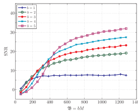
BPDN

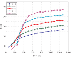
 IHT

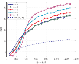
QIHT

Figure 2: Comparison between (from left to right) BPDN, IHT and QIHT for several quantization scenarios. The SNR is expressed in dB as a function of the bit budget $\mathfrak{B}$ and the number of bits $b$ used to quantize each measurement.

An extensive set of simulations has been designed for evaluating the efficiency of QIHT in comparison with two other methods more suited to high-resolution quantization, namely, IHT and BPDN. Our objective is to show that QIHT provides better quality results at least at small quantization levels. For all experiments, we set $N=1024$, $K=16$ and the $K$-sparse signals were generated by choosing their supports uniformly at random amongst the $N\choose K$ available ones, while their non-zero coefficients were drawn uniformly at random on the sphere $S^{K-1}\subseteq\mathbb{R}^{K}$. For each algorithm, $100$ initial such sparse vectors were generated and the reconstruction method was tested for $1\leq b\leq 5$ and for $\mathfrak{B}=bM\in\{64,128,\,\cdots,1280\}$, i.e., approximately fixing $M=\lfloor\mathfrak{B}/b\rfloor$. For each experimental condition, the quantized $M$-dimensional measurement vectors $\bm{y}_{b}$ was generated as in (2) with a random sensing matrix $\bm{\Phi}\sim\mathcal{N}^{M\times N}(0,1)$ and according to an optimal Lloyd-Max $b$-bits Quantizer $\mathcal{Q}_{b}$ (Sec. 3). IHT and QIHT iterations were both stopped at step $n$ as soon as ${\|\bm{x}^{(n+1)}-\bm{x}^{(n)}\|}{\|\bm{x}^{(n+1)}\|}^{-1}<10^{-4}$ or if $n=1000$. The BPDN algorithm was solved with the SPGL1 Matlab toolbox [21]. In IHT and QIHT, signal sparsity $K$ was assumed known and both were set with $\mu={\textstyle\frac{1}{M}}\big{(}1-\sqrt{\frac{2K}{M}}\big{)}$. This fits the IHT condition $\mu<1/(1+\delta_{2K})$ mentioned in Sec. 5 by assuming that the RIP radius $\delta_{2K}$ behaves like $\sqrt{2K/M}$, which is a common assumption in CS. For BPDN, the noise energy was given by an oracle installing BPDN in the best reconstruction scenario, i.e., $\epsilon=\|\bm{\Phi}\bm{x}_{0}-\bm{y}\|_{2}$. Whatever the reconstruction method, given an initial signal $\bm{x}_{0}\in\Sigma^{*}_{K}$ and its reconstruction $\bm{x}^{*}$, the reconstruction quality was measured by ${\rm SNR}(\bm{x}_{0},\bm{x}^{*})=-20\log_{10}\big{\|}\bm{x}_{0}\,-\,\|\bm{x}^{*}\|^{-1}\bm{x}^{*}\big{\|}$. In other words, we focus here on a good “angular” estimation of the signals, adopting therefore a common metric for $b>1$ and for $b=1$, where amplitude information is lost. Finally, for each method and each couple of $(M,b)$, the SNR was averaged over the 100 test signals and expressed in dB.

Fig. 2 gathers the SNR performances of the 3 methods as a function of $\mathfrak{B}$. QIHT outperforms both BPDN and IHT for the selected scenarios, especially for low bit quantizers. At high resolution, the gain between QIHT and IHT decreases as expected from the limit case analysis of QIHT. We can also notice that, first, there is almost no quality difference between QIHT at $b=1$ and $b=2$. This could be due to a non-optimality of the Lloyd-Max quantizer with respect to QIHT reconstruction error minimization. Second, BPDN and IHT asymptotically present the “$6$dB per bit” gain, while QIHT hardly exhibits such behavior only when $b=4\to 5$.

Finally, in order to test Prop. 2, the SNR reached by the single thresholding solution $\hat{\bm{x}}$ is plotted in dashed in Fig 2-right. Despite its poor behavior compared to QIHT at $b=1$, it outperforms BPDN at high $\mathfrak{B}=M$ with a ${\rm SNR}\geq 10$dB at $M=N=1024$. A curve fitting (no shown here) shows that this SNR increases a bit faster than $20\log_{10}\sqrt{K/M}+O(1)$.

7 Conclusion

We have introduced the QIHT algorithm as a generalization of the BIHT and IHT algorithms aiming at enforcing consistency with quantized observations at any bit resolution. In particular, we showed that the almost obvious inclusion of the quantization operator in the IHT recursion is actually related to the implicit minimization of a particular inconsistency cost $\mathcal{E}_{b}$. This function generalizes the one-sided $\ell_{1}$ cost of BIHT and asymptotically converges to the quadratic fidelity minimized by IHT. There is still a hard work to be performed in order to prove QIHT convergence and stability. However, the different ingredients defining it, as $\mathcal{E}_{b}$, deserve independent analysis extending previous $1$-bit embeddings developed in [11, 13, 12].

Appendix A Proximity of almost 1-bit consistent sparse vectors

The relation (7) is induced by the following theorem and by its subsequent Corollary 1. These use the normalized Hamming distance between two strings $\bm{a},\bm{b}\in\{-1,+1\}^{M}$ defined by $d_{H}(\bm{a},\bm{b})=\frac{1}{M}\sum_{i=1}^{M}a_{i}\oplus b_{i}$, where $\oplus$ is the XOR operation such that $a_{i}\oplus b_{i}$ equals 0 if $a_{i}=b_{i}$ and 1 otherwise. For shortening the notations, we define also $\bm{\varphi}(\bm{u}):={\rm sign}\,(\bm{\Phi}\bm{u})\in\{-1,+1\}^{M}$ for $\bm{u}\in\mathbb{R}^{N}$.

Theorem 1.

Let $\bm{\Phi}\sim\mathcal{N}^{M\times N}(0,1)$. Fix $r\leq M/2$, $0\leq\eta\leq 1$ and $0<\delta<1$. If the number of measurements $M$ satisfies

$$M-r\geq\tfrac{2}{\delta}\,\big{(}2K\,\log(N)+r\log(M)+4K\log(\tfrac{17}{\delta})+\log\tfrac{2e}{\eta}\big{)},$$ (9)

then,

$$\forall\bm{a},\,\bm{b}\in\Sigma^{*}_{K},\quad d_{H}\big{(}\bm{\varphi}(\bm{a}),\bm{\varphi}(\bm{b})\big{)}\leq\tfrac{r}{M}\quad\Rightarrow\quad\|\bm{a}-\bm{b}\|\leq\delta$$

with probability exceeding $1-\eta$.

This improves the previous theorem proved in [11].

Proof.

First, notice that if $M\,d_{H}\big{(}\bm{\varphi}(\bm{a}),\bm{\varphi}(\bm{b})\big{)}\leq r$, there exists a $\mathcal{T}\subset[M]$ with $|\mathcal{T}|\geq M-r$ such that $\bm{\varphi}_{\mathcal{T}}(\bm{a})=\bm{\varphi}_{\mathcal{T}}(\bm{b})$. Let $[M]_{r}$ be the set of subsets of $[M]$ whose size is bigger than $M-r$. Using a union bound argument, we have

$$\mathbb{P}\big{[}\ \exists\,\mathcal{T}\subset[M]_{r},\ \exists\,\bm{a},\bm{b}\in\Sigma^{*}_{K}:\ \bm{\varphi}_{\mathcal{T}}(\bm{a})=\bm{\varphi}_{\mathcal{T}}(\bm{b}),\ \|\bm{a}-\bm{b}\|>\delta\ \big{]}$$

$$\leq\bigcup_{\mathcal{T}\subset[M]_{r}}\mathbb{P}\big{[}\ \exists\,\bm{a},\bm{b}\in\Sigma^{*}_{K}:\ \bm{\varphi}_{\mathcal{T}}(\bm{a})=\bm{\varphi}_{\mathcal{T}}(\bm{b}),\ \|\bm{a}-\bm{b}\|>\delta\ \big{]}.$$ (10)

We know from [11, Theorem 2] that, as soon as

$$M^{\prime}\geq\tfrac{2}{\delta}\,\big{(}2K\,\log(N)+4K\log(\tfrac{17}{\delta})+\log{\textstyle\frac{1}{\eta}}\big{)},$$

the random generation of $\bm{\Phi}^{\prime}\sim\mathcal{N}^{M^{\prime}\times N}(0,1)$ fullfils

$$\mathbb{P}\big{[}\ \exists\bm{a},\bm{b}\in\Sigma^{*}_{K}:\ \bm{\varphi}^{\prime}(\bm{a})=\bm{\varphi}^{\prime}(\bm{b}),\ \|\bm{a}-\bm{b}\|>\delta\ \big{]}\ \leq\ \eta,$$

with $\bm{\varphi}^{\prime}(\cdot)={\rm sign}\,(\bm{\Phi}^{\prime}\cdot)$. Therefore, for a given $\mathcal{T}\subset[M]_{r}$ and by setting $\bm{\Phi}^{\prime}=(\operatorname{\bf Id}_{\mathcal{T}})^{T}\bm{\Phi}$, i.e., the matrix obtained by restricting $\bm{\Phi}$ to the rows indexed in $\mathcal{T}$, we have $\bm{\varphi}_{\mathcal{T}}=\bm{\varphi}^{\prime}$, $M^{\prime}=|\mathcal{T}|\geq M-r$ and

$$\mathbb{P}\big{[}\ \exists\,\bm{a},\bm{b}\in\Sigma^{*}_{K}:\ \bm{\varphi}_{\mathcal{T}}(\bm{a})=\bm{\varphi}_{\mathcal{T}}(\bm{b}),\ \|\bm{a}-\bm{b}\|>\delta\ \big{]}\leq\eta$$

if $M\geq r+\tfrac{2}{\delta}\,\big{(}2K\,\log(N)+4K\log(\tfrac{17}{\delta})+\log{\textstyle\frac{1}{\eta}}\big{)}$.

Under the same condition on $M$, and observing that, for $r\leq\lfloor M/2\rfloor$, $|[M]_{r}|=\sum_{k=0}^{r}{M\choose M-k}\leq(r+1){M\choose r}\leq(r+1)(eM/r)^{r}$, (10) provides

$$\mathbb{P}\big{[}\ \exists\,\mathcal{T}\subset[M]_{r},\ \exists\,\bm{a},\bm{b}\in\Sigma^{*}_{K}:\ \bm{\varphi}_{\mathcal{T}}(\bm{a})=\bm{\varphi}_{\mathcal{T}}(\bm{b}),\ \|\bm{a}-\bm{b}\|>\delta\ \big{]}\leq(r+1)(\tfrac{eM}{r})^{r}\,\eta.$$

Analyzing the complementary event and redefining $\eta\leftarrow(r+1)({eM}/{r})^{r}\,\eta$, we get finally

$$\mathbb{P}\big{[}\forall\,\bm{a},\bm{b}\in\Sigma^{*}_{K}:\ M\,d_{H}\big{(}\varphi_{\mathcal{T}}(\bm{a}),\bm{\varphi}_{\mathcal{T}}(\bm{b})\big{)}\leq r,\ \|\bm{a}-\bm{b}\|\leq\delta\ \big{]}$$

$$=\ \mathbb{P}\big{[}\ \forall\,\mathcal{T}\subset[M]_{r},\ \forall\,\bm{a},\bm{b}\in\Sigma^{*}_{K}:\ \bm{\varphi}_{\mathcal{T}}(\bm{a})=\bm{\varphi}_{\mathcal{T}}(\bm{b}),\ \|\bm{a}-\bm{b}\|\leq\delta\ \big{]}\geq 1-\eta,$$

as soon as

$$M\geq r+\tfrac{2}{\delta}\,\big{(}2K\,\log(N)+r\log(M)+4K\log(\tfrac{17}{\delta})+\log\tfrac{2e}{\eta}\big{)}.$$

∎

Corollary 1.

Let $\bm{\Phi}\sim\mathcal{N}^{M\times N}(0,1)$. Fix $r\leq M/2$, $0\leq\eta\leq 1$ and $0<\delta<1$. If the number of measurements $M$ satisfies

$$M\geq\tfrac{2}{\delta}\,\big{(}2K\log(\max(N,M))+4K\log(\tfrac{17}{\delta})+\log\tfrac{2e}{\eta}\big{)},$$

then,

$$\forall\bm{a},\,\bm{b}\in\Sigma^{*}_{K},\quad d_{H}(A(\bm{a}),A(\bm{b}))\leq\tfrac{r}{M}\quad\Rightarrow\quad\|\bm{a}-\bm{b}\|\leq\ \tfrac{K+r}{K}\,\delta$$

with probability exceeding $1-\eta$.

Proof.

The proof is obtained from Theorem 1 by redefining $\delta\leftarrow\tfrac{K+r}{K}\,\delta$, observing that $\frac{2}{\delta}\log M\geq 1$ if $M>1$ and by slightly enforcing the condition (9) on $M$. ∎

References

- [1] D. L. Donoho, “Compressed Sensing,” IEEE Trans. Inf. Th., 52(4):1289–1306, 2006.
- [2] E. J. Candès, J. Romberg and T. Tao. “Stable signal recovery from incomplete and inaccurate measurements,” Comm. Pure Appl. Math., 59(8):1207–1223, 2006
- [3] W. Dai, H. V. Pham, and O. Milenkovic, “Information theoretical and algorithmic approaches to quantized compressive sensing,” IEEE Trans. Comm., 59(7):1857–1866, 2011.
- [4] J. Laska, P. Boufounos, M. Davenport, and R. Baraniuk, “Democracy in action: Quantization, saturation, and compressive sensing,” App. Comp. Harm. Anal., 31(3): 429–443, 2011.
- [5] A. Zymnis, S. Boyd, and E. Candès, “Compressed sensing with quantized measurements,” IEEE Sig. Proc. Let., 17(2): 149–152, 2010.
- [6] L. Jacques, D. K. Hammond, and M. J. Fadili, “Dequantizing Compressed Sensing: When Oversampling and Non-Gaussian Constraints Combine.,” IEEE Trans. Inf. Th., 57(1): 559–571, 2011.
- [7] L. Jacques, D. K. Hammond, and M. J. Fadili, “Stabilizing nonuniformly quantized compressed sensing with scalar companders,” arXiv:1206.6003, 2012.
- [8] J. Z. Sun and V. K. Goyal, “Optimal quantization of random measurements in compressed sensing,” in Int. Symp. Inf. Th. (ISIT), June 2009.
- [9] C. Sinan Güntürk, M Lammers, A. M. Powell, R. Saab, and Ö. Yılmaz, “Sobolev duals for random frames and quantization of compressed sensing measurements,” Found. Comp. Math., 13(1):1–36, 2013.
- [10] P. Boufounos and R. Baraniuk, “1-bit compressive sensing,” in Proc. Conf. Inform. Sc. Sys. (CISS), Princeton, NJ, Mar. 2008.
- [11] L. Jacques, J.N. Laska, P.T. Boufounos, and R.G. Baraniuk, “Robust 1-bit compressive sensing via binary stable embeddings of sparse vectors,” IEEE Trans. Inf. Th., 59(4):2082-2102, 2013.
- [12] Y. Plan and R. Vershynin, “One-bit compressed sensing by linear programming,” Comm. Pure Appl. Math., 2013.
- [13] Y. Plan and R. Vershynin, “Robust 1-bit compressed sensing and sparse logistic regression: A convex programming approach,” IEEE Trans. Inf. Th., 59(1):482–494, 2013.
- [14] S. Bahmani, P. T. Boufounos and B. Raj, “Robust 1-bit Compressive Sensing via Gradient Support Pursuit,” arXiv:1304.6627, 2013.
- [15] Z. Yang, L. Xie, and C. Zhang, “Unified framework and algorithm for quantized compressed sensing,” arXiv:1203.4870, 2012.
- [16] T. Blumensath and M.E. Davies, “Iterative hard thresholding for compressed sensing,” App. Comp. Harm. Anal., 27(3):265–274, 2009.
- [17] S. S. Chen, D. L. Donoho, and M. A. Saunders, “Atomic Decomposition by Basis Pursuit,” SIAM J. Sc. Comp., 20(1):33–61, 1998.
- [18] T. Blumensath, “Accelerated iterative hard thresholding,” Sig. Proc., 92(3):752–756, 2012.
- [19] R. M. Gray and D. L. Neuhoff, “Quantization,” IEEE Trans. Inf. Th., 44(6):2325–2383, 1998.
- [20] R.T. Rockafellar, Convex analysis, vol. 28, Princeton Univ. Press, 1970.
- [21] E. van den Berg and M. P. Friedlander, “SPGL1: A solver for large-scale sparse reconstruction,” June 2007, http://www.cs.ubc.ca/labs/scl/spgl1.