A fully quantum mechanical calculation of the diffusivity of hydrogen in iron using the tight binding approximation and path integral theory

Abstract

We present calculations of free energy barriers and diffusivities as functions of temperature for the diffusion of hydrogen in $\alpha$-Fe. This is a fully quantum mechanical approach since the total energy landscape is computed using a new self consistent, transferable tight binding model for interstitial impurities in magnetic iron. Also the hydrogen nucleus is treated quantum mechanically and we compare here two approaches in the literature both based in the Feynman path integral formulation of statistical mechanics. We find that the quantum transition state theory which admits greater freedom for the proton to explore phase space gives result in better agreement with experiment than the alternative which is based on fixed centroid calculations of the free energy barrier. We also find results in better agreement compared to recent centroid molecular dynamics (CMD) calculations of the diffusivity which employed a classical interatomic potential rather than our quantum mechanical tight binding theory. In particular we find first that quantum effects persist to higher temperatures than previously thought, and conversely that the low temperature diffusivity is smaller than predicted in CMD calculations and larger than predicted by classical transition state theory. This will have impact on future modeling and simulation of hydrogen trapping and diffusion.

I Introduction

The damaging effect of hydrogen (H) on the mechanical properties of metals and alloys has been studied extensively since the 1940s. However, there is still considerable debate regarding the specific mechanisms for H-assisted damage, that is, the role of H in the fracture process. Various doubts exist regarding the validity of each of the existing H-assisted embrittlement mechanisms.Birnbaum and Sofronis (1994); Katz et al. (2001) It is widely accepted that combinations of several mechanisms can occur simultaneously and synergistically, since some involve common background processes. A common factor in all H-assisted damage mechanisms is the crucial role of H transport and trapping. In all cases, the predominant H-assisted damage mechanisms are dependent on the rate and mode of H transport.

In particular, H diffusion in Fe and Fe alloys is extremely important because it leads to engineering problems caused by H embrittlement and degradation of high-strength steels. Hydrogen in $\alpha$-Fe diffuses between tetrahedral sites of the perfect bcc lattice, the diffusivity being among the highest reported for any metal.Kiuchi and McLellan (1983); Hagi and Hayashi (1987); Hayashi et al. (1989); Nagano et al. (1982) This high H diffusivity results from the very low activation energies due to the quantum nature of H.Katz et al. (2001) The existence of microstructural imperfections (vacancies, solute atoms, dislocations, grain boundaries, etc.) introduces low energy trapping sites within the lattice which retard the overall diffusion rate.Kirchheim (1988, 1987); Kumnick and Johnson (1980) Because H is a light element, intrinsic processes in H diffusion are strongly influenced by its quantum mechanical behavior. At low temperatures quantum tunneling is expected to be the dominant mechanism. At high temperatures, the transition is dominated by classical jumping over the barrier. In order to understand the process of H diffusion in Fe it is essential to study H trapping and migration over the whole range of temperatures covering both the quantum and classical dominated regimes and the cross over between them.

The structure of the paper is as follows. In section II we introduce the classical methodologies which we modify in section III for the quantum nature of the diffusing particle. We show the results of our calculations in section IV in which we have combined the quantum transition state theoryVoth (1993) (QTST) for the first time with the method of Wang and Landau (WLMC) for the calculation of free energies.Wang and Landau (2001) This has the particular benefit that from a single Monte-Carlo simulation the free energy may be extracted at any temperature, in contrast to the usual Metropolis Monte-Carlo.Tuckerman (2010) Our results are demonstrated to be in excellent agreement with experiment, and since our combined QTST WLMC scheme is very compuationally efficient this opens the way to large scale simulations of trapping bt defects in steel. We make some concluding remarks in section V.

II Molecular dynamics and transition state theory

One of the most commonly adopted approximations in atomistic simulations of a system’s evolution is the assumption that atomic nuclei behave as classical particles. Theoretical approaches based on molecular dynamics (MD) have been used to study H trapping and migration in Fe.Taketomi et al. (2008); Matsumoto et al. (2009) An estimate of hydrogen diffusivity can also be provided by employing the kinetic Monte Carlo (kMC) method.Hoagland et al. (1998); Ramasubramaniam et al. (2008) The fundamental transition rate constants used by kMC can be estimated without knowledge of the dynamics of the system within the framework of the classical transition state theory (TST).Ramasubramaniam et al. (2008, 2009) Unfortunately, when simulations of H diffusion are made at or below room temperature significant deviations from classical behavior are to be expected due to the quantum nature of the proton motion. An explicit treatment of quantum effects is not only desirable for improvement of the accuracy of the simulations, but it can be essential for understanding phenomena and experimental observations depending directly on the quantum nature of the nuclear motion.

The state of the art for quantum treatment of the ionic degrees of freedom involves the use of the centroid path integral molecular dynamics (CMD) method.Cao and Voth (1993) This was used recently to evaluate the differences between the free energies of H at the interstitial and binding sites in $\alpha$-Fe.Kimizuka et al. (2011); Kimizuka and Ogata (2001) However, including quantum effects is computationally demanding compared to a simulation with classical nuclei, since one has to compute the energy of many replicas of the physical system. Studying H migration and calculations of the diffusivity in the presence of microstructural imperfections also require simulations in large blocks of atoms for times exceeding the typical CMD time scales.

The kMC method has the advantage of being computationally less expensive because the interatomic interactions are not computed directly from the electronic structure “on the fly” as the simulation proceeds. Instead, kMC uses precomputed transition rates along the minimal energy paths (MEP) between the metastable sites, thereby allowing employment of more precise electronic structure methods, density functional theory (DFT), tight binding (TB) or bond order potentials for computation the energy of the physical system and derivation of the transition rates. The application of kMC for the study of H diffusion permits simulations in larger blocks of atoms for periods of time significantly longer than one can achieve with direct MD simulation, which is essential for studying H migration and trapping in the presence of microstructural imperfections and consequent extraction of the diffusion coefficients.

Classical TST assumes that the H transition rates between metastable sites follow approximately the Arrhenius law and the activation energy is the difference of the energy for a fully relaxed system at the saddle point separating the stable sites and the stable site itself.Ramasubramaniam et al. (2008, 2009) Modern ab initio modeling provides a good description of the energetics and potential energy surface (PES) in Fe–H systems. However, these calculations of energy barriers can not account for quantum corrections arising from the low mass H atom. Although the overall energy barriers are small, as expected for a small atom like H and the geometry of the bcc lattice, they are significantly higher than the experimentally determined activation energies.Ramasubramaniam et al. (2008) A quantum treatment of the hydrogen degrees of freedom is mandatory to capture such effects.

III Feynman path integrals and quantum transition state theory

GillanGillan (1987a, b) has argued that the appropriate quantum generalization of the activated rate constant can be obtained using the Feynman path integral (PI) method.Feynman (1972) This generalization involves the ratio of probabilities for finding the centroid of the quantum chain at the saddle point and at the stable site. The activation energy is the difference of the free energy for a fully relaxed system with the the centroid at the saddle point separating the stable sites, and at the stable site itself. Gillan has also proposed a technique for calculation of this ratio in path integral simulation. Although Gillan’s approach allows one to examine the relative transition rates at different temperatures it does not yield an absolute value for the activated rate constant, A general TST like theory for calculation of the quantum activated rate constant providing expressions for both the quantum activation free energy and the prefactor was proposed by Voth Voth (1990); Voth and O’Gorman (1991); Li and Voth (1991); Voth (1993) Voth’s quantum transition state theory (QTST) presents the general quantum transition rate problem from the perspective of path integral centroid statistics.Feynman (1972)

In this paper, we study the activated dynamics of hydrogen diffusion between tetrahedral sites in $\alpha$-iron by employing Voth’s path integral formulation of quantum transition state theory for calculation of corresponding activation rate constants. Apart from allowing simulations in larger blocks of atoms for periods of time significantly longer than can be achieved with CMD simulation, the advantage of employing kMC with a transition rate determined by PI QTST for studying H diffusion is that one can use an accurate electronic structure approach for computation of the energy of the physical system and derivation of the quantum transition rates.

III.1 Interatomic forces and total energy

Recent work studying diffusion of interstitial H in $\alpha$-Fe by applying the CMD approachKimizuka et al. (2011); Kimizuka and Ogata (2001) employed an interatomic potential for describing the electronic structure of the Fe–H system within the embedded atom method (EAM) formalism.Mendelev et al. (2003) Although there is a large number of existing classical potentials,Baskes et al. (1997); Wen et al. (2001); Mendelev et al. (2003) which are certainly useful, they all suffer from a particular drawback in that the underlying classical EAM type models require a huge number of parameters needing to be fitted to a very large training set of data. This and the rather opaque functional form of the interatomic interactions in the classical potentials mean that while they are able to model many properties quantitatively they are at risk of failure once they are transferred into situations for which they were not fitted. A well known example of this is the failure of all but one of the many classical potentials for $\alpha$-Fe to simulate correctly the core structure of the screw dislocation; TB models do not suffer from this problem.

The electronic structure and interatomic forces in magnetic iron, both pure and containing hydrogen impurities, in the present calculations, have been described using a non orthogonal self consistent tight binding model.Paxton and Finnis (2008); Paxton and Elsässer (2010) The transferability of the model has been tested against known properties in many cases. Agreement with both observations and DFT calculations is remarkably good, opening up the way to quantum mechanical atomistic simulation of the effects of hydrogen in iron.Paxton and Elsässer (2010) By contrast with EAM potentials, the TB model used in this paper comprises a correct quantum mechanical description of both magnetism and the metallic and covalent bond.

III.2 Theory

The approach to a quantum mechanical TST, proposed by Voth, is based on Feynman’s formulation of quantum statistical mechanics.Feynman (1972) in which the partition function $Z$ of a particle moving in one dimension having Hamiltonian

$$H=\frac{p^{2}}{2m}+V(x)$$

and in equilibrium with a heat bath at inverse temperature $\beta=1/k_{B}T$ is written approximately using a discretization of the imaginary time Feynman path integral asGillan (1989)

$$Z\approx Z_{P}=\left(\frac{mP}{2\pi\beta\hbar^{2}}\right)^{\frac{P}{2}}\int dx_{1}...dx_{P}\,\,\exp\left\{-\beta\sum_{s=1}^{P}\left[\frac{1}{2}\frac{mP}{\hbar^{2}\beta^{2}}(x_{s+1}-x_{s})^{2}+P^{-1}V(x_{s})\right]\right\}$$ (1)

This expresses the remarkable mapping of the partition function of a quantum mechanical particle onto that of a necklace of $P$ beads connected by classical harmonic springs of stiffness $mP/\hbar^{2}\beta^{2}$, each bead feeling in addition a potential energy $V(r)/P$, for large $P$ much weaker than the true potental energy. Note also that the potential energy of the springs in the classical analog derives from the kinetic energy operator in the Hamiltonian. The numerical estimate converges to the quantum limit when the discretization parameter $P$ is chosen to be large enough. In the $P\rightarrow\infty$ limit, as Feynman shows, the partition function is written as a path integral

$$Z=\int{\cal D}x(\tau)\,e^{-S/\hbar}$$

which is an integral over all closed paths $x(\tau)$ in configuration space. The action integral is

$$S[x(\tau)]=\int_{0}^{\hbar\beta}{\rm d}\tau\left[\frac{1}{2}m\dot{x}^{2}(\tau)+V(x(\tau))\right]$$

The key to obtaining the rate constant in QTST is to separate out paths in the multidimensional coordinate space into a “reaction coordinate” denoted $q(\tau)$ and the remaining coordinates ${\bf r}(\tau)$.Voth (1993) $q(\tau)$ might be a path connecting two stable configurations through a saddle point, or it may be a path constrained to the dividing surface separating two stable configurations.Vineyard (1957) One can then work with a reduced centroid density

$$\rho_{c}(q_{c},\textbf{r}_{c})=\int{\cal D}q(\tau){\cal D}\textbf{r}(\tau)\delta(q_{c}-q_{0})\delta(\textbf{r}_{c}-\textbf{r}_{0})\exp\{-S[q(\tau),\textbf{r}(\tau)]/\hbar\}$$

in terms of which a constrained partition function is

$$Z_{c}(q^{*})=\int d\,\textbf{r}_{c}\,\rho(q^{*},\textbf{r}_{c})$$

where $q^{*}$ is the transition state value of the reaction coordinate. The “centroid” variable $q_{0}$ in path integration is defined along the $q$ direction by the expression

$$q_{0}=\frac{1}{\hbar\beta}\int_{0}^{\hbar\beta}d\tau q(\tau)$$

The transition rate constant $\kappa$ can then be expressed in terms of $Z_{c}(q^{*})$ as

$$\kappa^{\rm QTST}=\frac{\bar{v}}{2}\frac{Z_{c}(q^{*})}{Z_{R}}$$

where, $Z_{R}$ is the unconstrained “reactant” partition function for the particle localized about a lattice or trap site, and $\bar{v}$ is a velocity factorVoth (1993) which can be estimated by adopting a free particle dynamical model along the $q$ direction and taking the velocity from a Maxwell distribution. In this way, $\bar{v}$ becomes

$$\bar{v}_{FP}=\left(\frac{2}{\pi m\beta}\right)^{\frac{1}{2}}$$

and the quantum transition state rate constant is

$$\kappa^{\rm QTST}=\left(\frac{1}{2\pi m\beta}\right)^{\frac{1}{2}}\frac{Z_{c}(q^{*})}{Z_{R}}$$ (2)

This expression is difficult to implement in practice because in any numerical calculation via either molecular dynamics or Monte Carlo that generates a canonical distribution we do not have direct access to the partition function. It can be computed by generating a canonical distribution if it can be expressed in terms of averages of phase space functions. The QTST proton transfer rate constant may be re-expressed as Li and Voth (1991)

$$\kappa^{\rm QTST}=\nu\exp(-\beta\Delta F_{c})$$ (3)

where $\nu$ is the frequency of oscillation of the proton in the $q$ direction and the difference between centroid free energies of the reactant and transition state is

$$\Delta F_{c}=-k_{B}T\,\ln\left(\frac{Z_{c}(q^{*})}{Z_{c}(q_{R})}\right)$$ (4)

$q_{R}$ is the reactant state value of the reaction coordinate $q$. The free energy difference between the reactant and transition state can be evaluated using one of the methods for determination of the free energy profile along the reaction coordinate. An immediate disadvantage of the energy profile approaches is that it is necessary to perform many simulations of a system at physically uninteresting intermediate values. Only initial and final configurations correspond to actual physical states, and ultimately we can only attach physical meaning to the free energy difference between these two states. Nevertheless, the intermediate averages must be accurately calculated in order for the integration to yield a correct result. The number of physically uninteresting intermediate averages increases dramatically when one tries to derive the temperature dependence of the quantum transition rate constant. In this case, the free energy difference between the reactant and transition state has to be evaluated for each temperature under interest, because both path integral MD method Parrinello and Rahman (1984) and conventional Monte Carlo methods generate a canonical distribution at a given temperature.

III.3 Free energy calculation

In this paper, we use the Wang-Landau Monte Carlo (WLMC) algorithm Wang and Landau (2001) to calculate directly the partition functions participating in the QTST activation factor. The key idea of the WLMC method is to calculate the density of states $\Omega(E)$ directly by a random walk in energy space instead of performing a canonical simulation at a fixed temperature. The WLMC approach allows one to estimate various thermodynamic properties over a wide range of temperatures from a single simulation run. The canonical partition function can be expressed in terms of the density of states $\Omega(E)$ as

$$Z(\beta)=\int_{0}^{\infty}dE\,e^{-\beta E}\,\Omega(E)$$ (5)

The approach of Wang and Landau is to sample the density of states directly and, once known, calculate the partition function via (5).

The path integral form of the quantum partition function $Z_{P}(\beta)$ in the $P$-bead approximation (1) can be expressed as Vorontsov-Velyaminov and Lyubartsev (2003)

$$Z_{P}(\beta)=\left(\frac{mP}{2\pi\beta\hbar^{2}}\right)^{\frac{P}{2}}\int d\textbf{r}\exp\left(-\frac{S_{1}(\textbf{r})}{\beta}-\beta S_{2}(\textbf{r})\right)$$

which reveals that the quantum partition function depends on two temperature independent functions

$$S_{1}({\bf r}) =\sum_{s=1}^{P}\frac{mP}{2\hbar^{2}}({\bf r}_{s+1}-{\bf r}_{s})^{2}$$

$$S_{2}({\bf r}) =\sum_{s=1}^{P}(P^{-1}V({\bf r}_{s}))$$

$S_{1}({\bf r})$ is related to the kinetic energy of the system and $S_{2}({\bf r})$ accounts for the potential energy. Hence the density of states, which is an analogue of the classical density of states function, would depend on two variables, $s_{1}$ and $s_{2}$ Vorontsov-Velyaminov and Lyubartsev (2003)

$$\Omega(s_{1},s_{2})=\int{\rm d}{\bf r}\,\delta(s_{1}-S_{1}({\bf r}))\,\delta(s_{2}-S_{2}({\bf r}))$$ (6)

Then we can express $Z$ as

$$Z(\beta)=\int_{0}^{\infty}ds_{1}ds_{2}\,\exp(-\frac{s_{1}}{\beta}-\beta s_{2})\,\Omega(s_{1},s_{2})$$

With this density of states the partition function that describes the thermodynamics of the quantum system can be calculated for any temperature. However, we can determine the density of states only up to a multiplicative constant, $\Omega_{0}$, since this will not change the relative measures at different energy levels. The uncertainty in the density of states leads to a multiplicative uncertainty in the quantum transition rate (2). The quantum transition rate at a given temperature can be derived independently from (3) by using a method for determination of free energy difference between the transition and reactant states. If one knows $\kappa^{\rm QTST}$ at a given temperature, the multiplicative constant can be determined from (2) and (3) by comparison of the corresponding transition rates at the same temperature. In the present work we calculate the free energy difference appearing in (3) by using an extension of the Wang-Landau sampling scheme to the problem of the free energy profile along reaction coordinates.Calvo (2002) If the process of transition is monitored by a switching variable $q$, the free energy profile is

$$F(q)=-k_{B}T\,\ln P(q)$$ (7)

where $P(q)$ is the probability density that the system is in a state with reaction coordinate $q$. Since $\Omega(E)$ and $P(q)$ play similar roles the Wang-Landau sampling scheme can be used to generate a function that approaches the probability $P(q)$ over many Monte Carlo passes with the following Metropolis acceptance rule:

$$\hbox{acc}(\textbf{r}_{c}^{\rm old}\rightarrow\textbf{r}_{c}^{\rm new})=\hbox{min}\left[1,\frac{\rho_{c}^{\rm new}(q,\textbf{r}_{c})}{\rho_{c}^{\rm old}(q,\textbf{r}_{c})}\frac{g(q^{\rm old})}{g(q^{\rm new})}\right]$$

where $g$ is the Wang-Landau scaling parameter.Calvo (2002) The multiplicative constant $\Omega_{0}$ can also be determined if the quantum transition rate (2) at high temperature (the classical limit) is approximated by a transition rate determined by the classical TST.

IV Calculation of the hydrogen diffusivity in iron

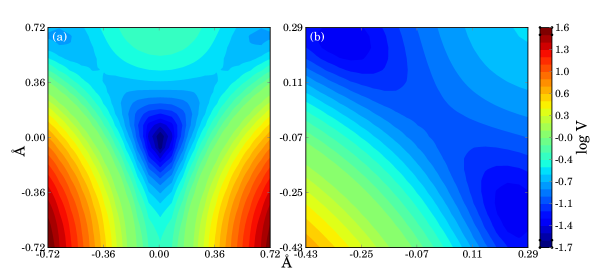
Figure 1: (color online) Potential energy surfaces for a H atom moving into the fixed atomic positions of the Fe atoms; (a) configuration in which the Fe atoms have been relaxed around a H atom in the tetrahedral “reactant” site; (b) the Fe atoms are relaxed around a H atom held at the saddle point position between two neighboring tetrahedral sites.

Here we study the real time quantum dynamics of hydrogen diffusion in perfect $\alpha$-iron by employing the path integral (PI) approach described above combined with WLMC. The electronic structure and interatomic forces in magnetic iron, both pure and containing hydrogen impurities, in the present calculations have been described using a non orthogonal self consistent tight binding model.Paxton and Elsässer (2010); Paxton and Finnis (2008) It is to be noted that the TB model predicts, correctly, that the configuration with the lowest potential energy is the tetrahedral site. The minimum energy path (MEP) and the transition state between two adjacent tetrahedral sites have been identified by using the nudged elastic band (NEB) method.Henkelman et al. (2000) In order to use the PI-WLMC technique to calculate corresponding partition functions, we constructed 3D potential energy surfaces (PESs) for the hydrogen motion in two fixed lattice configurations, corresponding to fully relaxed lattice of 16 Fe atoms with H atom in tetrahedral and saddle point configurations. We constructed PESs in these fixed lattice configurations by performing a large set of TB total energy calculations corresponding to different positions of the hydrogen nucleus. In all these calculations the nuclei are treated as classical point particles. The calculated potential energy surfaces are shown in figure 1

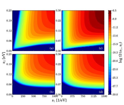
Figure 2: (color online) Density of states $\Omega(s_{1},s_{2})$ (6) for the proton moving in the potential of fixed Fe atoms as shown in figure 1; (a) centroid fixed at tetrahedral site; (b) centroid in the vicinity of tetrahedral site; (c) centroid fixed at the saddle point; (d) centroid on the dividing surface in the region of the barrier top. (a) and (c) are those used in Gillan’s theory in which the centroids are fixed at reactant and saddle point positions. (b) and (d) are appropriate to Voth’s method; in (b) the centroid is allowed to explore phase space in the region of the tetrahedral lattice site and in (d) the centroid is confined to the Vineyard dividing surface that intersects the saddle point.

We have studied the importance of quantum effects in hydrogen diffusion in perfect bcc-Fe by employing both Gillan’s approach for calculation of the activation energy and Voth’s formulation of path integral QTST. Our main result is the calculation of the density of states (6) at the stable state and in the region of the barrier top of a Fe–H system in the cases of Gillan’s formulation of the activation barrier and Voth’s PI QTST generalization of transition state theory. With these densities of states (DOS) the corresponding partition functions, describing the thermodynamics of the quantum system, can be calculated for any temperature. Knowing corresponding partition functions, we can determine a number of thermodynamic variables for the Fe–H system as functions of the temperature. The DOS of the stable and transition states as they are defined in both Gillan’s approach and path integral QTST are shown in figure 2

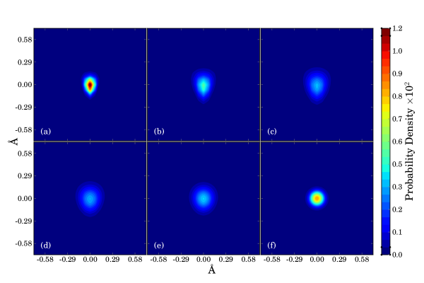
Figure 3: (color online) Position probability density (PPD) of the hydrogen nucleus when the centroid is fixed at tetrahedral site at temperature of (a) $T=$20K; (b) $T=$50K; (c) $T=$100K; (d) $T=$200K; (e) $T=$ 300K; (f) $T=$1000K. In each panel the tetrahedral site is located at the center of the image. Note that at high temperature the PPD is spherical and located close to the centroid as expected of a classical particle. At intermediate lower temperatures the PPD spreads out, but at the lowest temperature the PPD contracts due to the freezing of the proton into its lowest oscillator state; however it is no longer spherical as it “feels” the low symmetry of the tetrahedral site.

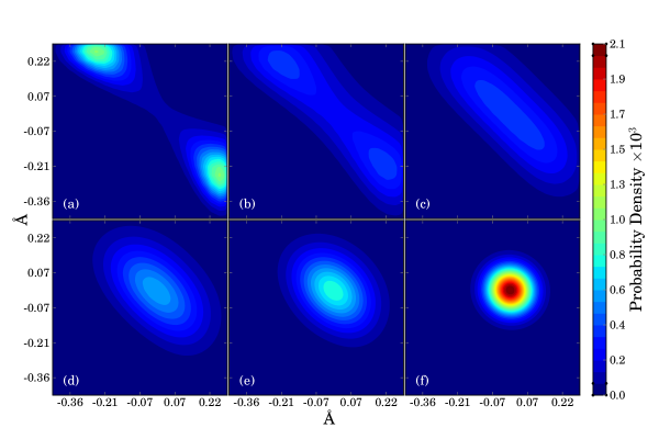
Figure 4: (color online) Position probability density of the hydrogen nucleus when the centroid is fixed at the saddle pointe at temperature of (a) $T=$20K; (b) $T=$50K; (c) $T=$100K; (d) $T=$200K; (e) $T=$ 300K; (f) $T=$1000K. In each panel the saddle point is at the center of the image and there is a symmetry equivalent tetrahedral site at the upper left and lower right corners. Note how, at low temperature the proton “splits into two” and even though the centroid of the chain of “beads” is held fixed at the saddle point the greatest position probability density is close to the energy minima at the tetrahedral “reactant” sites.

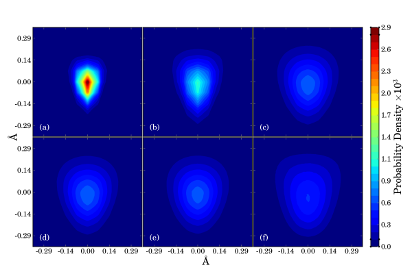
Figure 5: (color online) Position probability density of the hydrogen nucleus when the centroid is in the vicinity of tetrahedral site at temperature of (a) $T=$20K; (b) $T=$50K; (c) $T=$100K; (d) $T=$200K; (e) $T=$300K; (f) $T=$1000K. In each panel the tetrahedral site is located at the center of the image. In comparison to figure 3 the particle is more spread out even at the highest temperature. This reflects the greater degree of freedom of the PI QTST theory compared to the method of Gillan.

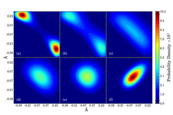
Figure 6: (color online) Position probability density (PPD) of the hydrogen nucleus when the centroid is on the dividing surface in the region of the barrier top at temperature of (a) $T=$20K; (b) $T=$50K; (c) $T=$100K; (d) $T=$200K; (e) $T=$ 300K; (f) $T=$1000K. As remarked in the caption to figure 5 the PPD is greatly spread out compared to that in the Gillan formulation of the path integral method. In addition, especially at high temperatures it is seen that the reduced density is allowing the proton to explore the phase space along the Vineyard dividing surface, which is “perpendicular” to the reaction path. As the centroid is no longer constrained to remain at the saddle point the resulting free energy barrier is larger and the diffusivity smaller in Voth’s method.

We also determine the position probability density of the hydrogen nucleus (proton) when it is in tetrahedral and saddle point configurations. In Gillan’s path integral procedure H is in stable or transition states when the centroid of the imaginary time reaction coordinate path is in a stable interstitial impurity site (figure 3) or a saddle point between two neighboring interstitial sites (figure 4). Within Voth’s formulation of QTST, we determine the position probability density of the hydrogen nucleus when its centroid is confined in the potential well of tetrahedral sites (figure 5) and on the dividing surface that intersects the classical saddle point between two such sites (figure 6). The probability distributions as functions of temperature, when the centroid is at the transition state, are shown in figure 4 and figure 6. It is very clear that in both cases at low temperature the proton in the transition state “splits into two” with greatest position probability density not at the saddle point but very close to the tetrahedral sites. At low temperatures the transition rate is dominated by quantum tunneling through the barrier and both Gillan’s and Voth’s approaches predict similar results. In the classical limit (high temperature) the hydrogen atom can be considered as a classical particle and its position probability density is concentrated in the vicinity of the potential well and classical saddle point. At high temperature, the reduced centroid density $Z_{c}(q^{*})$ and the reactant partition function $Z_{R}$ of a Fe–H system in a stable tetrahedral site can be approximated by the configurational partition functions of a classical particle existing in quasi equilibrium. The assumption that the motion of atoms in both configurations can be treated as simple harmonic oscillators leads to the familiar Vineyard–Slater expression,Vineyard (1957) derived from many body transition state theory. Hence, the position probability density of the hydrogen nucleus calculated in the framework of path integral QTST (figures 5 and 6) includes corrections due to motion (thermal “vibration”) of the proton near the stable state and in the region of the barrier top. As seen from the comparison between figure 3 and figure 5, as well as between figure 4 and figure 6, these corrections are significant at room temperature and at high temperature.

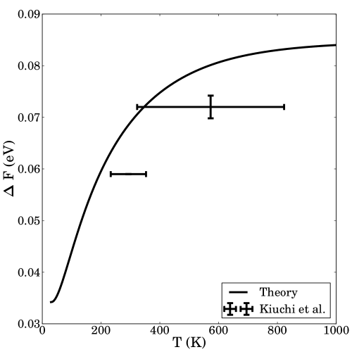
Figure 7: The free energy needed to carry the H atom from an initial stable position to a transition state as a function of temperature, obtained using Gillan’s approach. The activation energy is compared with assessments from hydrogen equilibration and permeation tests in ref. [Kiuchi and McLellan, 1983].

In order to determine the activation barrier height given by Gillan’s approach and the PI QTST transition rate as a function of temperature we have calculated the corresponding partition functions appearing in both methods in the temperature interval between 20 and 1000K. Since the DOS are determined by a WLMC path integral approach up to a multiplicative constant, we apply the extension of Wang-Landau sampling to the problem of the free energy profile to obtain the corresponding probability distribution functions $P(q)$ at a fixed temperature of 1000K. We find that Gillan’s free energy difference between stable and transition states is $\Delta F=0.084$eV at 1000K. As is to be expected this value is very close to the classical limit of the migration barrier ($E_{m}=0.088$eV) because quantum corrections are negligible at high temperatures. After determination of the corresponding multiplicative constant, $\Omega_{0}$, we can calculate the free energy needed to carry the H atom from an initial stable position to a transition state in the temperature interval between 20 and 1000K. The activation energy, defined by Gillan’s quantum generalization, as a function of temperature is shown in figure 7.

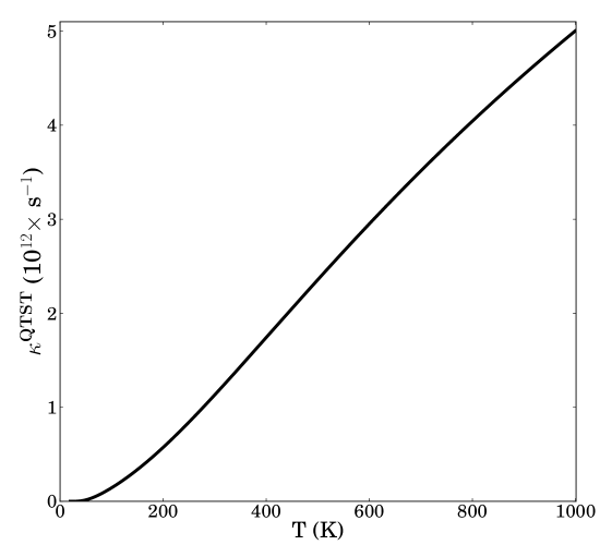
Figure 8: Quantum transition rate calculated by PI QTST in the temperature interval 20–1000K.

The free energy difference between transition and reaction states at 1000K, given in Voth’s theory by the ratio between the corresponding reduced centroid densities (4), is calculated by using WLMC to obtain the free energy profile (7). We find that the free energy needed to carry a H atom from a stable to a transition state at 1000 K is 0.087eV. The proton transition rate at 1000K is determined from (3). The value of frequency of oscillation of the proton in the $q$ direction, $\nu=1.29\times 10^{13}$s^-1, appearing in (3) is derived from a harmonic fit to the energy along the reaction coordinate determined by NEB TB calculations. After calculation of the multiplicative constant $\Omega_{0}$ we can find the temperature dependence of the quantum transition rate between two tetrahedral sites in $\alpha$-Fe in the interval between 20 and 1000K (see figure 8). This is the primary goal of the current work.

In the simple case of H diffusion in a perfect bcc lattice, the diffusion coefficient $D$ can be determined from the Einstein formula assuming an uncorrelated random walk in cubic symmetry

$$D=\frac{1}{6}zR^{2}\kappa^{\rm QTST}$$

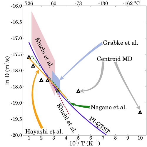
Figure 9: (color online) Diffusion coefficients of H in $\alpha$-Fe in the temperature range 100–1000 K calculated by PI QTST (blue line). The pink band of data represents an assessment by Kiuchi and McLellanKiuchi and McLellan (1983) of hydrogen gas equilibration experiments. The solid red and green lines are data from electrochemical permeation experiments, assessed in ref. [Kiuchi and McLellan, 1983] and measured in ref. [Nagano et al., 1982] respectively. The blue band of data are measurements by Grabke and RiekeGrabke and Rieke (2000) and the yellow line shows measurements by Hayashi et al.Hayashi et al. (1989) The triangles show theoretical results from centroid molecular dynamics calculations using a classical interatomic potential and are taken from ref. [Kimizuka et al., 2011]. Note that these are in less good agreement with experiment at high temperature compared to our fully quantum mechanical predictions and that at low temperatures the CMD method predicts diffusivities significantly larger than ours. This may reflect the difficulty in Metropolis Monte Carlo sampling at low temperature in contrast to the WLMC method which accesses all temperatures as a result of a single sampling.

where $z=4$ is the number of neighboring positions and $R=a^{2}/8$ is the jump distance. An Arrhenius plot of the diffusion coefficient as a function of temperature in the interval 20 to 1000K is shown in figure 9. Diffusion coefficients determined at different temperatures by kMC using the same $k^{\rm QTST}$ confirm the results obtained from the Einstein formula. For comparison, experimental diffusivities over a wide temperature range (240–-1000K)Nagano et al. (1982); Kiuchi and McLellan (1983); Hagi and Hayashi (1987); Hayashi et al. (1989) and diffusion coefficients calculated by the centroid molecular dynamics (CMD) methodKimizuka et al. (2011); Cao and Voth (1993) at several temperatures between 100 and 1000K are also plotted in figure 9. Our results are in very reasonable agreement with the experimental measurements. A deviation from linear behavior is observed in the Arrhenius plots based on our PI QTST results. Also, they are in good agreement with the diffusion coefficients calculated by using computationally demanding centroid molecular dynamics techniqueKimizuka et al. (2011) in the interval 300–1000K, while at low temperatures these data show a much larger diffusivity. It should be noted that in view of the logarithmic axis in figure 9 our quantum mechanical tight binding predictions are in better agreement even at high temperature with those using an energy landscape based in a classical interatomic potential. Our PI QTST results are in excellent agreement with the experimental measurements below 300 K, where CMD predicts larger diffusion coefficients.

V Concluding remarks

Our kMC path integral QTST approach in combination with WLMC, along with the TB model describing energy of the Fe–H system, permits a description of real time quantum dynamics of hydrogen diffusion in $\alpha$-iron over a wide temperature range. Unlike conventional MD and Monte Carlo methods generating canonical distributions, and computationally demanding centroid MD techniques, the WLMC algorithm allows one directly to calculate the partition functions participating in the PI QTST transition rates over a wide range of temperatures from a single simulation run. The results reveal that quantum effects play a crucial role in the process of H migration even at room temperature. Although Gillan’s quantum generalization of the activated rate constant describes correctly quantum tunneling at low temperatures, the thermal “vibrations” of the proton at the saddle point are not accounted for within this approach, which leads to an underestimation of the activation barrier height at room and high temperatures. The diffusion coefficient as a function of temperature, calculated using the QTST rate constant determined by PI WLMC, is in good agreement with the experimentally evaluated diffusivity in the interval 240–-1000K.

The computationally less expensive kMC method using precomputed PI QTST transition rates calculated by WLMC technique, proposed in this article, opens the way to studying the quantum dynamics of hydrogen migration and trapping in presence of microstructural imperfections and calculation of the diffusion coefficients over a wide temperature range.

References

- Birnbaum and Sofronis (1994) H. K. Birnbaum and P. Sofronis, Mat. Sci. Eng. A 176, 191 (1994).
- Katz et al. (2001) Y. Katz, N. Tymiak, and W. W. Gerberich, Eng. Fract. Mech. 68, 619 (2001).
- Kiuchi and McLellan (1983) K. Kiuchi and R. B. McLellan, Acta Metall. 31, 961 (1983).
- Hagi and Hayashi (1987) H. Hagi and Y. Hayashi, Trans. Jpn. Inst. Met. 28, 368 (1987).
- Hayashi et al. (1989) Y. Hayashi, H. Hagi, and A. Tahara, Z. Phys. Chem. (Neue Folge) 164, 815 (1989).
- Nagano et al. (1982) M. Nagano, Y. Hayashi, N. Ohtani, M. Isshiki, and K. Igaki, Scr. Met. 16, 973 (1982).
- Kirchheim (1988) R. Kirchheim, Prog. Mat. Sci. 32, 261 (1988).
- Kirchheim (1987) R. Kirchheim, Acta Met. 35, 271 (1987).
- Kumnick and Johnson (1980) A. Kumnick and H. Johnson, Acta Met. 28, 33 (1980).
- Voth (1993) G. A. Voth, J. Phys. Chem. 97, 8365 (1993).
- Wang and Landau (2001) F. Wang and D. P. Landau, Phys. Rev. Lett. 86, 2050 (2001).
- Tuckerman (2010) M. E. Tuckerman, Statistical Mechanics: Theory and Molecular Simulation, (OUP, 2010).
- Taketomi et al. (2008) S. Taketomi, R. Matsumoto, and N. Miyazaki, J. Mat. Sci 43, 1166 (2008).
- Matsumoto et al. (2009) R. Matsumoto, S. Taketomi, S. Matsumoto, and N. Miyazaki, Int. J. Hydrogen Energy 34, 9576 (2009).
- Hoagland et al. (1998) R. G. Hoagland, A. F. Voter, and S. M. Foiles, Scr. Mat. 39, 589 (1998).
- Ramasubramaniam et al. (2008) A. Ramasubramaniam, M. Itakura, M. Ortiz, and E. Carter, J. Mat, Sci. 23, 2757 (2008).
- Ramasubramaniam et al. (2009) A. Ramasubramaniam, M. Itakura, and E. A. Carter, Phys. Rev. B 79, 174101 (2009).
- Cao and Voth (1993) J. Cao and G. A. Voth, J. Chem. Phys. 99, 10070 (1993).
- Kimizuka et al. (2011) H. Kimizuka, H. Mori, and S. Ogata, Phys. Rev. B 83, 094110 (2011).
- Kimizuka and Ogata (2001) H. Kimizuka and S. Ogata, Phys. Rev. B 84, 024116 (2001).
- Gillan (1987a) M. J. Gillan, Phys. Rev. Lett. 58, 563 (1987a).
- Gillan (1987b) M. J. Gillan, J. Phys. C: Solid State Phys. 20, 3621 (1987b).
- Feynman (1972) R. P. Feynman, Statistical Mechanics—a set of lectures (Benjamin, Reading, Mass., 1972).
- Voth (1990) G. A. Voth, Chem. Phys. Lett. 170, 289 (1990).
- Voth and O’Gorman (1991) G. A. Voth and E. V. O’Gorman, J. Chem. Phys. 94, 7342 (1991).
- Li and Voth (1991) D. Li and G. A. Voth, J. Chem. Phys. 95, 10425 (1991).
- Mendelev et al. (2003) M. I. Mendelev, S. Han, D. J. Srolovitz, G. J. Ackland, D. Y. Sun, and M. Asta, Phil. Mag. 83, 3977 (2003).
- Baskes et al. (1997) M. I. Baskes, X. Sha, J. E. Angelo, and N. R. Moody, Modell. Simul. Mater. Sci. Eng. 5, 651 (1997).
- Wen et al. (2001) M. Wen, X.-J. Xu, S. Fukuyama, and K. Yokogawa, J. Mat. Res. 16, 3496 (2001).
- Paxton and Finnis (2008) A. T. Paxton and M. W. Finnis, Phys. Rev. B 77, 024428 (2008).
- Paxton and Elsässer (2010) A. T. Paxton and C. Elsässer, Phys. Rev. B 82, 235125 (2010).
- Gillan (1989) M. J. Gillan, in NATO ASI on Computer Modelling of Fluids, Polymers and Solids, edited by R. Catlow, S. C. Parker, and M. P. Allen (Springer, Berlin, 1989).
- Vineyard (1957) G. H. Vineyard, J. Phys. Chem. Solids 3, 121 (1957).
- Parrinello and Rahman (1984) M. Parrinello and A. Rahman, J. Chem. Phys. 80, 860 (1984).
- Vorontsov-Velyaminov and Lyubartsev (2003) P. N. Vorontsov-Velyaminov and A. P. Lyubartsev, J. Phys. A: Math. Gen. 36, 685 (2003).
- Calvo (2002) F. Calvo, Mol. Phys. 100, 3421 (2002).
- Henkelman et al. (2000) G. Henkelman, B. Uberuaga, and H. Jónsson, J. Chem. Phys. 113, 9901 (2000).
- Grabke and Rieke (2000) H. J. Grabke and E. Rieke, Materiali in Tehnologije 34, 331 (2000).