Topological surface states in paramagnetic and antiferromagnetic iron pnictides

Abstract

The electronic structure of iron pnictides is topologically nontrivial, leading to the appearance of Dirac cones in the band structure for the antiferromagnetic phase. Motivated by the analogy with Dirac cones in graphene, we explore the possible existence of topologically protected surface states. Surprisingly, bands of surface states exist even in the paramagnetic state. A realistic five-orbital model predicts two such bands. In the antiferromagnetic phase, these surface bands survive but split. We obtain the bulk and surface dispersion from exact diagonalization of two- and five-orbital models in a strip geometry and discuss the results based on topology.

I Introduction

Two of the most active areas in condensed matter physics concern the iron pnictidesJoh10 ; DHD12 and topological properties of matter.HaK10 ; QiZ11 The iron pnictides are of interest since they show multiband superconductivity with high transition temperatures competing with itinerant antiferromagnetism. Topology in condensed matter has received a lot of attention in part because nontrivial topology can induce surface or edge states. This paper is concerned with the topological properties and surface states of iron pnictides.

In iron pnictides, several iron $3d$ orbitals contribute significantly to the electronic states close to the Fermi energy. Ran et al.RWZ09 have realized that this multiorbital character can lead to nontrivial topological properties. They find band touchings at the $(0,0)$ and $(\pi,\pi)$ points in the Brillouin zone (BZ), which are associated with winding numbers in orbital space. As a consequence, the formation of a spin-density wave (SDW) with ordering vector $\mathbf{Q}=(\pi,0)$ cannot open a full gap but rather leaves an even number of Dirac points.RWZ09 This holds both for a two-orbital model including only the most important $3d_{YZ}$ and $3d_{ZX}$ orbitalsRQL08 and for a model including all five $3d$ orbitals.KOA08 While the two-orbital model does not give a realistic description, it allows a simpler discussion of the topological properties. On the other hand, the five-orbital modelKOA08 gives a good account of the low-energy band structure of the prototypical compound $\mathrm{LaFeAsO}$ and also leads to reasonable predictions for the magnetic order vs. doping.BDT11 ; SBT12 Evidence for the Dirac points has been obtained from quantum-oscillation experiments,HaS09 magnetotransportPBC13 and angle-resolved photoemission (ARPES).RNS10 ; HTT11 However, conflicting evidence is presented in TKT11, .

Dirac points in the band structure have attracted a lot of attention in the context of graphene.CGP09 There, Dirac points emerge due to the two-sublattice structure of the honeycomb lattice. They are accompanied by dispersing edge states at so-called zigzag edges,FWN96 ; RyH02 ; CGP06 ; CGP09 which appear in the 1D edge BZ between the projections of the Dirac points. Regardless of the different origins of the Dirac points, one may ask whether they have similar consequences in pnictides and in graphene. Specifically, do surface states also exist in the SDW phase of the iron pnictides? Yang and KeeYaK10 have indeed found surface bands for a two-orbital model with broken symmetry. However, the required combined orbital, SDW, and charge-density-wave order is not realized in iron pnictides and actually opens a full gap without Dirac points.

We will show that dispersing bands of surface states exist even in the paramagnetic phase of the iron pnictides, due to its topological character. In the SDW phase, the surface bands split. This is found for both two-orbital and five-orbital models but the latter features two surface bands, whereas the former has only one. We will explain the topological origin of the surface states.

II Models and method

We follow Refs. KOA08, ; RWZ09, in choosing $3d$ orbitals with respect to the $X$ and $Y$ axes of the tetragonal lattice, which are rotated by $45^{\circ}$ relative to the $x$ and $y$ axes of the square iron lattice. The two-orbital modelRQL08 ; RWZ09 retains only these two orbitals in a single-iron unit cell. The Hamiltonian is $H=H_{0}+H_{I}$, where the non-interacting part for the extended system reads $H_{0}=\sum_{\mathbf{k}\sigma}\sum_{a,b=1}^{2}d^{\dagger}_{\mathbf{k}a\sigma}\mathcal{H}_{ab}(\mathbf{k})d_{\mathbf{k}b\sigma}$. Here, $\mathcal{H}(\mathbf{k})$ is a $2\times 2$ matrix in orbital space,

$$\mathcal{H}(\mathbf{k})=2t_{1}\,(\cos k_{x}-\cos k_{y})\,\tau^{1}$$ (1)

$${}-2(t_{2}-t_{2}^{\prime})\,\sin k_{x}\sin k_{y}\,\tau^{3}$$

$${}+[2(t_{2}+t_{2}^{\prime})\,\cos k_{x}\cos k_{y}+2t_{1}^{\prime}\,(\cos k_{x}+\cos k_{y})]\,\tau^{0},\quad$$

where $\tau^{1}$, $\tau^{2}$, $\tau^{3}$ are Pauli matrices, $\tau^{0}$ is the unit matrix, and the orbital index $1$ corresponds to $3d_{ZX}$ and $2$ to $3d_{YZ}$. We adopt the hopping parametersRWZ09 $t_{1}=0.30\,\mathrm{eV}$, $t_{1}^{\prime}=0.06\,\mathrm{eV}$, $t_{2}=0.51\,\mathrm{eV}$, and $t_{2}^{\prime}=0.09\,\mathrm{eV}$.

For the interactions we takeRWZ09

$$H_{I} = \frac{U}{2}\sum_{\mathbf{i}}(\hat{n}_{\mathbf{i}1}^{2}+\hat{n}_{\mathbf{i}2}^{2})+(U-2J)\sum_{\mathbf{i}}n_{\mathbf{i}1}n_{\mathbf{i}2}$$ (2)

$${}+J\sum_{\mathbf{i}}\sum_{\sigma\sigma^{\prime}}d_{\mathbf{i}1\sigma}^{\dagger}d_{\mathbf{i}2\sigma^{\prime}}^{\dagger}d_{\mathbf{i}1\sigma^{\prime}}d_{\mathbf{i}2\sigma}$$

$${}+J\sum_{\mathbf{i}}(d_{\mathbf{i}1\uparrow}^{\dagger}d_{\mathbf{i}1\downarrow}^{\dagger}d_{\mathbf{i}2\downarrow}d_{\mathbf{i}2\uparrow}+\mathrm{H.c.}),$$

where $\hat{n}_{\mathbf{i}a}\equiv\sum_{\sigma}d_{\mathbf{i}a\sigma}^{\dagger}d_{\mathbf{i}a\sigma}$, and the interaction parameters are chosen as $U=1.20\,\mathrm{eV}$ and $J=0.12\,\mathrm{eV}$. Assuming a SDW with ordering vector $\mathbf{Q}=(\pi,0)$ and spins pointing along the $S_{z}$ axis, a mean-field decoupling with $\langle d_{\mathbf{i}a\sigma}^{\dagger}d_{\mathbf{i}b\sigma}\rangle=n_{ab}+(-1)^{i_{x}}\,\frac{\sigma}{2}\,m_{ab}$ gives the mean-field Hamiltonian

$$H_{\mathrm{MF}}=H_{0}+\sum_{\mathbf{i}ab}(-1)^{i_{x}}M_{ab}\big{(}d_{\mathbf{i}a\uparrow}^{\dagger}d_{\mathbf{i}b\uparrow}-d_{\mathbf{i}a\downarrow}^{\dagger}d_{\mathbf{i}b\downarrow}\big{)},$$ (3)

with $M_{11}=-(Um_{11}+Jm_{22})/2$, $M_{22}=-(Um_{22}+Jm_{11})/2$, $M_{12}=M_{21}=-Jm_{21}$. The Hartree shifts $n_{ab}$ have been absorbed into $H_{0}$. The parameters $m_{ab}$ are calculated self-consistently, assuming half filling.

Edge states will be studied for a strip of width $W$ with (10) edges. Since the strip is extended along the $y$ axis, $k_{y}$ is a good quantum number and we carry out a Fourier transformation in the $y$ direction, $d_{\mathbf{i}a\sigma}=N_{y}^{-1/2}\sum_{k_{y}}e^{ik_{y}i_{y}}d_{i_{x}k_{y}a\sigma}$. The mean-field Hamiltonian then consists of blocks of dimensions $2W\times 2W$ for fixed $k_{y}$, $\sigma$. These blocks are diagonalized numerically, giving the energy bands of the strip system. We here assume that the SDW in the strip is described by the same order parameters $m_{ab}$ as for the extended system.

The five-orbital modelKOA08 includes all hopping amplitudes larger than $10\,\mathrm{meV}$ up to fifth neighbors. The hopping amplitudes and onsite energies are obtained from density-functional calculations and are tabulated in Ref. KOA08, . The interaction $H_{I}$ is analogous to the two-orbital model, except that the interorbital terms in Eq. (2) now become sums over all pairs of orbitals $a$, $b$, with $a<b$, where $a,b=1,\ldots,5$ correspond to $3d_{3Z^{2}-R^{2}}$, $3d_{ZX}$, $3d_{YZ}$, $3d_{X^{2}-Y^{2}}$, $3d_{XY}$. The interaction parameters are chosen to be $U=1.0\,\mathrm{eV}$ and $J=0.2\,\mathrm{eV}$.RWZ09 Applying a mean-field decoupling as above, we obtain the mean-field Hamiltonian (3), where now the orbital indices traverse $a,b=1,\ldots,5$, and $M_{aa}=-(Um_{aa}+J\sum_{b\neq a}m_{bb})/2$ and $M_{ab}=M_{ba}=-Jm_{ab}$ for $a\neq b$. The mean-field parameters $m_{ab}$ are determined self-consistently, assuming $6$ electrons per iron, corresponding to zero doping. For the (10) strip, we proceed analogously to the two-orbital case. By means of a Fourier transformation in the $y$ direction, the problem is reduced to the diagonalization of $5W\times 5W$ Hamiltonian matrices for fixed $k_{y}$, $\sigma$.

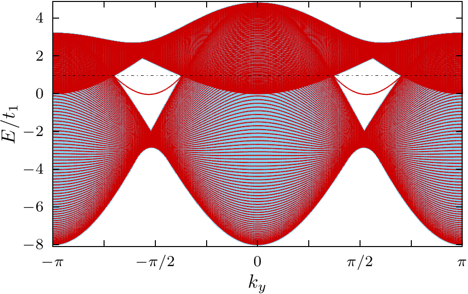
Figure 1: (Color online) Energy bands of the two-orbital model in the absence of SDW order: Bands of a (10) strip of width $W=100$ (medium red/gray lines) compared to the bulk bands projected onto the 1D BZ for the strip (light blue/gray region). Note the bands of edge states for the strip.

III Results and discussion

First, we consider the two-orbital model without SDW order, i.e., with $m_{ab}=0$, in a (10) strip geometry. In Fig. 1, we compare the energy bands of the (10) strip of width $W=100$ to the bands of the extended system projected onto the (10) edge BZ. All energies are twofold spin degenerate. We see that the majority of the bands of the strip lie within the projected continuum of bulk bands. However, there is an additional band that does not agree with the bulk continuum. We have found that the corresponding states are localized at the edges of the strip. A closer look reveals that this band, ignoring spin degeneracy, actually comprises two bands, which are only approximately degenerate. For finite widths $W$, the two states at given $k_{y}$ correspond to bonding and antibonding combinations of states localized at the two edges. Thus, there is a finite splitting, invisible in Fig. 1, which decreases exponentially with increasing $W$.

Figure 2: (Color online) Fermi surfaces (solid lines) in the BZ for the two-orbital model superimposed on the vector field $(\cos\phi_{\mathbf{k}},\sin\phi_{\mathbf{k}})$ (small arrows) showing the nontrivial winding of the Hamiltonian $\mathcal{H}(\mathbf{k})$ in orbital space. The black arrow denotes the BZ for an effective 1D model obtained by fixing $k_{y}$, where the arrow is meant to indicate the projection onto the 1D edge BZ.

The origin of the edge states can be understood from a topological argument. We start from the noninteracting first-quantized Hamiltonian $\mathcal{H}(\mathbf{k})$ of Eq. (1). We consider one spin sector throughout and suppress the spin index. For the strip, $k_{y}$ is a constant of motion. For each fixed value of $k_{y}$, we obtain an effective 1D model. For an extended system, the BZ of this 1D model is the subset with $k_{y}=\mathrm{const}$ of the 2D BZ. If the 1D BZ does not cross any Fermi surface, the 1D model is gapped in the bulk. One such 1D BZ is shown by the black arrow in Fig. 2. $\mathcal{H}(\mathbf{k})$ can be written asRWZ09

$$\mathcal{H}(\mathbf{k})=a(\mathbf{k})\,\tau^{0}+b(\mathbf{k})\,(\sin\phi_{\mathbf{k}}\,\tau^{1}+\cos\phi_{\mathbf{k}}\,\tau^{3}),$$ (4)

with $b(\mathbf{k})\geq 0$. The vector field $(\cos\phi_{\mathbf{k}},\sin\phi_{\mathbf{k}})$ is plotted in Fig. 2. It exhibits vortices with vorticities $\pm 2$ at the band-touching points $\mathbf{k}=(0,0)$ and $(\pi,\pi)$. Furthermore, a winding number of $+1$ ($-1$) is aquired when moving from $k_{x}=-\pi$ to $k_{x}=+\pi$ along a line with constant $k_{y}>0$ ($k_{y}<0$). The effective 1D system thus has a nontrivial topological structure in orbital space.RWZ09

The appearance of edge states is best understood by deforming the Hamiltonian of the effective 1D system into one with a topologically protected winding number. For fixed $k_{y}>0$ ($k_{y}<0$ is analogous), we deform the Hamiltonian into $\tilde{\mathcal{H}}(k_{x})=\cos k_{x}\,\tau^{1}-\sin k_{x}\,\tau^{3}$. This deformation does not change the topology of the bands and, in particular, leaves the energy gap open. $\tilde{\mathcal{H}}(k_{x})$ is unitarily equivalent to

$$\hat{\mathcal{H}}(k_{x})\equiv e^{-i\frac{\pi}{4}\tau^{1}}\tilde{\mathcal{H}}(k_{x})\,e^{i\frac{\pi}{4}\tau^{1}}=\left(\begin{array}[]{cc}0&e^{-ik_{x}}\\ e^{ik_{x}}&0\end{array}\right).$$ (5)

In the bulk, this new Hamiltonian has the eigenvalues $\pm 1$ for every $k_{x}$, i.e., it has flat bands. Furthermore, $\hat{\mathcal{H}}(k_{x})$ is time-reversal symmetric. The antiunitary time-reversal operator $T$ can be written as $T=KU_{T}$, where $K$ is the complex conjugation in our basis and $U_{T}$ is unitary and must satisfy $U_{T}\hat{\mathcal{H}}^{*}(-k_{x})U_{T}^{\dagger}=\hat{\mathcal{H}}(k_{x})$, which is fulfilled for $U_{T}=\tau^{0}$. Note that $T$ squares to $T^{2}=\tau^{0}$. $\hat{\mathcal{H}}(k_{x})$ is also charge-conjugation symmetric. The antiunitary charge-conjugation operator $C$ can be written as $C=KU_{C}$, where $U_{C}$ is unitary and must satisfy $U_{C}\hat{\mathcal{H}}^{*}(-k_{x})U_{C}^{\dagger}=-\hat{\mathcal{H}}(k_{x})$, which is fulfilled for $U_{C}=\tau^{3}$. We find $C^{2}=K\tau^{3}K\tau^{3}=\tau^{0}$. These symmetry properties imply that the deformed 1D model belongs to the Altland-Zirnbauer class BDI.Zir96 This class allows a $\mathbb{Z}$ topological invariant in 1D.SRF08

For the strip, the effective 1D model is a finite chain of length $W$. The $\mathbb{Z}$ topological invariant means that states localized at the ends can exist, but does not guarantee that $\hat{\mathcal{H}}(k_{x})$ has any. However, this is easily seen by transforming $\hat{\mathcal{H}}(k_{x})$ into real space, which gives $\hat{H}=\sum_{j=1}^{W-1}(d_{j+1,\uparrow}^{\dagger}d_{j,\downarrow}+d_{j,\downarrow}^{\dagger}d_{j+1,\uparrow})$, where ${\uparrow}$, ${\downarrow}$ now refer to the orbital pseudospin. The ${\uparrow}$ (${\downarrow}$) state at $j=1$ ($j=W$) is not coupled to any other state. Thus there are two zero-energy states localized at the ends. These arguments can be made for any $k_{y}$ for which the 1D BZ does not intersect a Fermi surface.

What does this tell us about the original Hamiltonian $\mathcal{H}(\mathbf{k})$ with fixed $k_{y}$? That Hamiltonian has neither $T$ nor $C$ symmetry and is thus in class A, which is topologically trivial in 1D. Our point is that the original Hamiltonian can be obtained from $\hat{\mathcal{H}}(k_{x})$ by a continuous deformation without closing the gap. During the deformation, the $T$ and $C$ symmetries are lost so that the zero-energy end states are no longer protected. However, the energy of the end states evolves smoothly during the deformation. Hence, for $\mathcal{H}(\mathbf{k})$ there are still two edge states for every $k_{y}$ for which the effective 1D Hamiltonian is gapped. These states have no reason to be at zero energy and will generally have an exponentially small overlap with each other, which splits their energies. In principle, the edge states are not protected against merging with the bulk continuum. However, we find separate edge states wherever the bulk is gapped, presumably due to level repulsion between edge and bulk states. Note the similarity to graphene: The edge band at graphene zigzag edges is a flat zero-energy band only for a model without next-nearest-neighbor hopping. In real graphene, it is dispersing.CGP06 ; CGP09

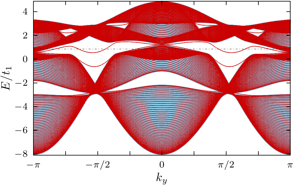
Figure 3: (Color online) Energy bands of the two-orbital model with SDW order: Bands of a (10) strip of width $W=100$ (medium red/gray lines) compared to the bulk bands projected onto the 1D BZ for the strip (light blue/gray region).

In the presence of a SDW with ordering vector $\mathbf{Q}=(\pi,0)$, the unit cell of the iron square lattice is doubled in the $x$ direction. Therefore, the bands are folded into the magnetic BZ. SDW formation opens gaps at some of the new band crossings but not at all of them—the bands still stick together at Dirac points.RWZ09 Figure 3 shows the band structure of the (10) strip compared to the projected bulk bands. Spin degeneracy is not lifted by the SDW since the mean-field Hamiltonian is invariant under combined spin rotation and spatial reflection $x\to-x$. However, the near degeneracy between bonding and antibonding combinations of edge states is strongly broken. We instead find two edge states per spin direction, which are localized mainly at one edge and are split in energy due to the opposite exchange field at the two edges. Note that the edge bands are connected to the bulk bands at the projected Dirac points, similar to graphene. Moreover, Fig. 3 shows that additional edge bands appear within the new gaps away from the Fermi energy.

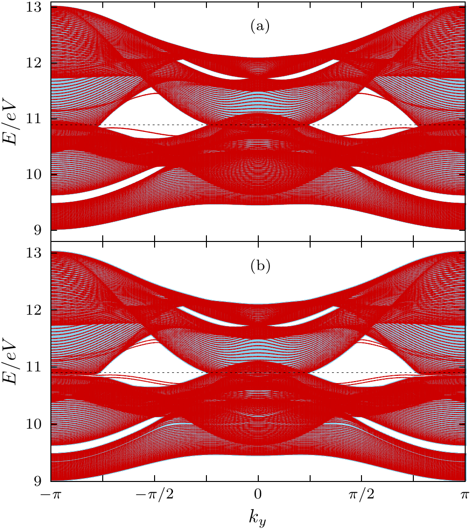
Figure 4: (Color online) Energy bands of the five-orbital model (a) without and (b) with SDW order: Bands of a (10) strip of width $W=60$ (medium red/gray lines) compared to the bulk bands projected onto the 1D BZ for the strip (light blue/gray regions).

To check whether the edge bands also occur for the five-orbital model,KOA08 ; RWZ09 we plot in Fig. 4 the energy bands of the (10) strip compared to the projected bulk bands for the paramagnetic and the SDW phase. In the paramagnetic phase we now find two edge bands, each of which is twofold spin degenerate and, in the wide limit, also twofold degenerate between bonding and antibonding combinations. SDW order again leads to the opening of gaps at crossings of folded bands. The twofold spin degeneracy remains but the asymptotic degeneracy between bonding and antibonding states is lifted, for the same reason as for the two-orbital model.

To understand the appearance of surface states in the five-orbital model, we again consider effective gapped 1D models obtained by fixing $k_{y}$ to values for which the path through the BZ at constant $k_{y}$ does not intersect a Fermi surface. In this case, two bands lie above the Fermi energy and three below. The Hamiltonian can be deformed continuously without closing the gap performing the following steps. (i) The hopping amplitudes between the $d_{3Z^{2}-R^{2}}$ and all other orbitals are tuned to zero and the resulting decoupled band is shifted down in energy, effectively removing it from the model, together with two electrons per iron. (ii) The hopping amplitudes beyond next-nearest neighbors are tuned to zero. All components of the Hamiltonian $\mathcal{H}(k_{x})$ can now be written as linear combinations of $\cos k_{x}$, $\sin k_{x}$, and a constant. (iii) All constant terms are tuned to zero. (iv) The coefficients of $\sin k_{x}$ in the diagonal components are tuned to zero. (v) The coefficients of $\cos k_{x}$ in the off-diagonal components are tuned to zero. (vi) The remaining coefficients in diagonal components are tuned to unity and in off-diagonal components to $1/\sqrt{2}$. A unitary transformation in orbital space maps the resulting Hamiltonian onto

$$\hat{\mathcal{H}}(k_{x})=\left(\begin{array}[]{cccc}0&e^{-ik_{x}}&0&0\\ e^{ik_{x}}&0&0&0\\ 0&0&0&e^{-ik_{x}}\\ 0&0&e^{ik_{x}}&0\end{array}\right).$$ (6)

Since this deformed Hamiltonian just consists of two copies of the Hamiltonian in Eq. (5), it has two sets of zero-energy end states of distinct orbital character. Upon deforming the Hamiltonian back into the original one, the end states for every considered $k_{y}$ continuously develop into dispersing bands. In addition, the degeneracy between the edge states of different orbital character is lifted so that we end up with two bands.

IV Conclusions

We have shown that two models of iron pnictides predict the existence of dispersing bands of surface states at (100) surfaces for the paramagnetic state. They could be used to probe the topologically nontrivial electronic structure. These bands are twofold spin degenerate and have an additional twofold degeneracy in the limit of a thick slab due to the decoupling of the states localised at the two surfaces. The main difference between the two-orbital and the five-orbital model is that the latter predicts two instead of one such bands. Their existence can be understood from a topological argument based on the continuous deformation of the Hamiltonian into one in Altland-Zirnbauer class BDI. In the SDW state, where we had guessed from an analogy to graphene that surface states might exist, the surface bands split into two twofold degenerate bands. It should be noted that while the two models inherit the surface states from topologically nontrivial Hamiltonians, they are not themselves topologically nontrivial. Hence, the surface states are not robust against disorder scattering. The analogy is thus more with graphene than with topological insulators.

The origin of the surface states discussed here is completely different from surface states at (001) surfaces of iron pnictides of the 1111 family, such as $\mathrm{LaOFeAs}$, which have been observed by ARPES.LYM09 ; ELK10 In this case, surface bands result from the polar nature of these surfaces.ELK10 Surface states of this kind are not expected for $\mathrm{LiFeAs}$ and $\mathrm{NaFeAs}$ since the (001) surface of these compounds is not polar and they are indeed not seen by ARPES.LKB10 ; YLM12

The surface states predicted here could be detected by ARPES or scanning tunneling spectroscopy on (100) surfaces, which are however challenging to prepare. An alternative could be tunneling into the edges of thin (001) films, either using an STM tip, a technique that has been successful for the detection of edge states in graphene,KFE05 or one of the setups discussed in Ref. Sei11, in the context of Josephson junctions. Such tunneling experiments would probe the density of states, which is expected to be enhanced close to (100) edges of the film. In particular, the van Hove singularities associated with extrema of the surface bands lead to an enhancement of the density of states since the surface states are essentially one-dimensional. It is an interesting question what happens to the surface states when superconductivity sets in. Superconductivity of the $s^{+-}$ type preferred for iron pnictides could introduce energy gaps in the surface bands discussed here but also induce additional surface-bound states.OnT09 Both would also be relevant for recent suggestions to engineer topological superconductors by using the proximity effect of superconducting iron pnictides.ZKM13

References

- (1) D. Johnston, Adv. Phys. 59, 803 (2010).
- (2) P. Dai, J. Hu, and E. Dagotto, Nature Phys. 8, 709 (2012).
- (3) M. Z. Hasan and C. L. Kane, Rev. Mod. Phys. 82, 3045 (2010).
- (4) X.-L. Qi and S.-C. Zhang, Rev. Mod. Phys. 83, 1057 (2011).
- (5) Y. Ran, F. Wang, H. Zhai, A. Vishwanath, and D.-H. Lee, Phys. Rev. B 79, 014505 (2009).
- (6) S. Raghu, X.-L. Qi, C.-X. Liu, D. J. Scalapino, and S.-C. Zhang, Phys. Rev. B 77, 220503(R) (2008).
- (7) K. Kuroki, S. Onari, R. Arita, H. Usui, Y. Tanaka, H. Kontani, and H. Aoki, Phys. Rev. Lett. 101, 087004 (2008).
- (8) P. M. R. Brydon, M. Daghofer, and C. Timm, J. Phys.: Condens. Matter 23, 246001 (2011).
- (9) J. Schmiedt, P. M. R. Brydon, and C. Timm, Phys. Rev. B 85, 214425 (2012).
- (10) N. Harrison and S. E. Sebastian, Phys. Rev. B 80, 224512 (2009); M. Sutherland, D. J. Hills, B. S. Tan, M. M. Altarawneh, N. Harrison, J. Gillett, E. C. T. O’Farrell, T. M. Benseman, I. Kokanovic, P. Syers, J. R. Cooper, and S. E. Sebastian, Phys. Rev. B 84, 180506(R) (2011).
- (11) I. Pallecchi, F. Bernardini, F. Caglieris, A. Palenzona, S. Massidda, and M. Putti, Eur. Phys. J. B 86, 338 (2013).
- (12) P. Richard, K. Nakayama, T. Sato, M. Neupane, Y.-M. Xu, J. H. Bowen, G. F. Chen, J. L. Luo, N. L. Wang, X. Dai, Z. Fang, H. Ding, and T. Takahashi, Phys. Rev. Lett. 104, 137001 (2010).
- (13) K. K. Huynh, Y. Tanabe, and K. Tanigaki, Phys. Rev. Lett. 106, 217004 (2011).
- (14) T. Terashima, N. Kurita, M. Tomita, K. Kihou, C.-H. Lee, Y. Tomioka, T. Ito, A. Iyo, H. Eisaki, T. Liang, M. Nakajima, S. Ishida, S. Uchida, H. Harima, and S. Uji, Phys. Rev. Lett. 107, 176402 (2011).
- (15) A. H. Castro Neto, F. Guinea, N. M. R. Peres, K. S. Novoselov, and A. K. Geim, Rev. Mod. Phys. 81, 109 (2009).
- (16) M. Fujita, K. Wakabayashi, K. Nakada, and K. Kusakabe, J. Phys. Soc. Jpn. 65, 1920 (1996); K. Nakada, M. Fujita, G. Dresselhaus, and M. S. Dresselhaus, Phys. Rev. B 54, 17954 (1996).
- (17) A. H. Castro Neto, F. Guinea, and N. M. R. Peres, Phys. Rev. B 73, 205408 (2006).
- (18) S. Ryu and Y. Hatsugai, Phys. Rev. Lett. 89, 077002 (2002).
- (19) B.-J. Yang and H.-Y. Kee, Phys. Rev. B 82, 195126 (2010), in particular note Fig. 7.
- (20) M. R. Zirnbauer, J. Math. Phys. 37, 4986 (1996); A. Altland and M. R. Zirnbauer, Phys. Rev. B 55, 1142 (1997).
- (21) A. P. Schnyder, S. Ryu, A. Furusaki, and A. W. W. Ludwig, Phys. Rev. B 78, 195125 (2008).
- (22) D. H. Lu, M. Yi, S.-K. Mo, J. G. Analytis, J.-H. Chu, A. S. Erickson, D. J. Singh, Z. Hussain, T. H. Geballe, I. R. Fisher, and Z.-X. Shen, Physica C 469, 452 (2009).
- (23) H. Eschrig, A. Lankau, and K. Koepernik, Phys. Rev. B 81, 155447 (2010).
- (24) A. Lankau, K. Koepernik, S. Borisenko, V. Zabolotnyy, B. Büchner, J. van den Brink, and H. Eschrig, Phys. Rev. B 82, 184518 (2010).
- (25) M. Yi, D. H. Lu, R. G. Moore, K. Kihou, C.-H. Lee, A. Iyo, H. Eisaki, T. Yoshida, A. Fujimori, and Z.-X. Shen, New J. Phys. 14, 073019 (2012).
- (26) Y. Kobayashi, K.-i. Fukui, T. Enoki, K. Kusakabe, and Y. Kaburagi, Phys. Rev. B 71, 193406 (2005); Y. Kobayashi, K.-i. Fukui, T. Enoki, and K. Kusakabe, Phys. Rev. B 73, 125415 (2006).
- (27) P. Seidel, Supercond. Sci. Technol. 24, 043001 (2011).
- (28) S. Onari and Y. Tanaka, Phys. Rev. B 79, 174526 (2009).
- (29) F. Zhang, C. L. Kane, and E. J. Mele, Phys. Rev. Lett. 111, 056402 (2013).