Entanglement as an indicator of a geometrical crossover in a two-electron quantum dot in a magnetic field

Abstract

We found that a downwardly concave entanglement evolution of the ground state of a two-electron axially symmetric quantum dot testifies that a shape transition from a lateral to a vertical localization of two electrons under a perpendicular magnetic field takes place. Although affected, the two-electron probability density does not exhibit any prominent change.

Quantum phase transitions (QPTs) in many-body systems, driven by quantum fluctuations at zero temperature, attract a considerable attention in recent years Sad . They are recognized as abrupt changes of the ground state of many-body system with varying a non-thermal control parameter (magnetic field, pressure etc) in the Hamiltonian of the system. Although the phases should be characterized by different types of quantum correlations on either side of a quantum critical point (actual transition point), in some cases they cannot be distinguished by any local order parameter. Particular examples are the integer and fractional quantum Hall liquids Hall which cannot be understood in terms of the traditional description of phases based on symmetry breaking and local order parameters. Nowadays, there is a growing interest in using quantum entanglement measures for study such transitions am and, in general, quantum correlations in many-body systems TMB2011 .

According to a general wisdom, various phases could exist in mesoscopic systems such as quantum dots (QDs) at different strengths of the applied magnetic field. Indeed, if an axially-symmetric QD is placed under a perpendicular magnetic field, one observes the orbital momentum and spin oscillations of the ground state of a QD by increasing the field strength RM . At certain field range the oscillations disappear and it is believed that the electrons form a finite-size analogue of infinite integer quantum Hall liquid. This fully polarized state in a QD is called the maximum density droplet. It is widely accepted that a further increase of the magnetic field should lead to the formation of the Wigner molecule, a finite-size analogue of the Wigner crystallization of the homogeneous electron gas. While the rotational symmetry of the ground state is expected to be preserved at the transition between these phases, specific excited (rotational) states should appear after the transition point RM ; mak ; yan . These states are not observed yet, and one needs further to develope experimental as well as theoretical tools to detect such transitions which may be associated with QPTs. Although finite systems can only show precursors of the QPT behaviour, they are also important for the development of the concept.

Two-electron QDs being realistic non-trivial systems are, in particular, attractive. In contrast to many-electron QDs, their eigenstates can be obtained very accurately, or in some cases exactly (cf kais ; r1 ). In fact, two-electron QDs become a testing ground for various approaches used for description of many-electron QDs. We will show that a quantum entanglement enables us to detect a geometrical (shape) transition in the ground state of two interacting electrons confined in a three-dimensional (3D) quantum dot under a magnetic field. It turns out that such a transition might be associated with a quantum phase transition.

We carry our analysis by means of the numerical diagonalization of the Hamiltonian

$$H=\sum_{j=1}^{2}\bigg{[}\frac{1}{2m^{*}\!}\,\Big{(}{\bf p}_{j}\!-\!\frac{e}{c}{\mathbf{A}}_{j}\Big{)}^{\!2}+U({\mathbf{r}}_{j})\bigg{]}+\frac{k}{|\mathbf{r}_{1}\!-\!\mathbf{r}_{2}|}+H_{\mathrm{spin}}.$$ (1)

Here $k=e^{2}/4\pi\varepsilon_{0}\varepsilon_{r}$ and $H_{\it spin}=g^{*}\mu_{B}(\mathbf{s}_{1}+\mathbf{s}_{2})\!\cdot\!\mathbf{B}$ describes the Zeeman term, where $\mu_{B}=|e|\hbar/2m_{e}c$ is the Bohr magneton. As an example, we will use the effective mass $m^{*}=0.067m_{e}$, the relative dielectric constant $\varepsilon_{r}=12$ and the effective Landé factor $g^{*}=-0.44$ (bulk GaAs values). For the perpendicular magnetic field we choose the vector potential with gauge ${\mathbf{A}}=\frac{1}{2}\mathbf{B}\times\mathbf{r}=\frac{1}{2}B(-y,x,0)$. The confining potential is approximated by a 3D axially-symmetric harmonic oscillator $U(\mathbf{r})=m^{*}[\omega_{0}^{2}\,(x^{2}\!+y^{2})+\omega_{z}^{2}z^{2}]/2$, where $\hbar\omega_{z}$ and $\hbar\omega_{0}$ are the energy scales of confinement in the $z$-direction and in the $xy$-plane, respectively.

Introducing the center of mass (CM) and relative coordinates: $\mathbf{R}=\frac{1}{2}(\mathbf{r}_{1}+\mathbf{r}_{2})$ and $\mathbf{r}_{12}=\mathbf{r}_{1}-\mathbf{r}_{2}$, – one separates the Hamiltonian (1) into the CM and relative motion terms $H=H_{\rm CM}+H_{\rm rel}$ (the Kohn theorem kohn ). The CM term is described by the oscillator Hamiltonian with the mass ${\cal M}=2m^{*}$ and frequencies of the one-particle confining potential $U$. The Hamiltonian for relative motion in cylindrical coordinates takes the form

$$H_{\rm rel}=\frac{1}{2\mu}\Big{(}p_{\rho_{12}}^{2}\!+\frac{\ell_{z}^{2}}{\rho_{12}^{2}}+p_{z_{12}}^{2}\!\Big{)}+\frac{\mu}{2}(\Omega^{2}\rho_{12}^{2}+\omega_{z}^{2}z_{12}^{2})+\frac{k}{r_{12}}-\omega_{L}\ell_{z},$$ (2)

where $\mu=m^{*}/2$ is the reduced mass, $\ell_{z}$ ($\to-i\hbar\partial/\partial\varphi$) is the projection of angular momentum for relative motion and $\rho_{12}=(x_{12}^{2}+y_{12}^{2})^{1/2}$, $\varphi=\arctan(y_{12}/x_{12})$, $r_{12}=(\rho_{12}^{2}+z_{12}^{2})^{1/2}$. Here, $\omega_{L}=|e|B/2m^{*}\!c$ is the Larmor frequency, and the effective lateral confinement frequency $\Omega=(\omega_{L}^{2}+\omega_{0}^{2})^{1/2}$ depends through $\omega_{L}$ on $B$.

The total two-electron wave function $\Psi(\mathbf{r}_{1},\mathbf{r}_{2})=\psi(\mathbf{r}_{1},\mathbf{r}_{2})\chi(\sigma_{1},\sigma_{2})$ is a product of the orbital $\psi(\mathbf{r}_{1},\mathbf{r}_{2})$ and spin $\chi(\sigma_{1},\sigma_{2})$ wave functions. Due to the Kohn theorem, the orbital wave function is factorized as a product of the CM and the relative motion wave functions $\psi(\mathbf{r}_{1},\mathbf{r}_{2})=\psi_{\mathrm{CM}}(\mathbf{R})\,\psi_{\mathrm{rel}}(\mathbf{r}_{12})$. The parity of $\psi_{\mathrm{rel}}(\mathbf{r}_{12})$ is a good quantum number as well as the magnetic quantum number $m$, since $\ell_{z}$ is the integral of motion.

The CM eigenfunction is a product of the Fock-Darwin state (the eigenstate of a single electron in an isotropic 2D harmonic oscillator potential in a perpendicular magnetic field) Fock in the $(X,Y)$-plane and the oscillator function in the $Z$-direction (both sets for a particle of mass ${\cal M}$). In this paper we consider the lowest CM eigenstate with the projection of CM angular momentum equal zero.

Since the Coulomb interaction ($k\neq 0$) couples the motions in $\rho_{12}$ and $z_{12}$-directions, the eigenfunctions of the Hamiltonian for relative motion (2) are expanded in the basis of the Fock-Darwin states $\Phi_{n,m}(\rho_{12},\varphi_{12})$ and oscillator functions in the $z_{12}$-direction $\phi_{n_{z}}(z_{12})$ (for a particle of mass $\mu$), i.e.

$$\psi_{\mathrm{rel}}(\mathbf{r}_{12})=\sum_{n,n_{z}}c_{n,n_{z}}^{(m)}\Phi_{n,m}(\rho_{12},\varphi_{12})\,\phi_{n_{z}}(z_{12}).$$ (3)

The coefficients $c_{n,n_{z}}^{(m)}$ can be determined by diagonalizing the Hamiltonian (2) in the same basis. Evidently, in numerical analysis the basis is restricted to a finite set $\{\Phi_{n,m}\,\phi_{n_{z}}|\,n=0,\ldots,n_{\max};\,n_{z}=0,\ldots,n_{z}^{\max}\}$. It must be, however, large enough to provide a good convergence for the numerical results.

For non-interacting electrons the ground state is described by the wave function $\psi_{\mathrm{rel}}=\Phi_{0,0}\,\phi_{0}$. For interacting electrons, however, the ground state (in the form (3)) evolves from $m=0$ to higher values of $m$ as the magnetic field strength increases. Since the quantum number $m$ and the total spin are related by expression $S=\frac{1}{2}[1-(-1)^{m}]$, this evolution leads to the well known singlet-triplet (S-T) transitions wag . Note that the Zeeman splitting (with $g^{*}<0$) lowers the energy of the $M_{S}=1$ component of the triplet states, while leaving the singlet states unchanged. As a consequence, the ground state is characterized by $M_{S}=S$.

At the value $\omega_{L}^{\mathrm{sph}}=(\omega_{z}^{2}-\omega_{0}^{2})^{1/2}$ the magnetic field gives rise to the spherical symmetry $(\omega_{z}/\Omega=1)$ in the axially-symmetric two-electron QD (with $\omega_{z}>\omega_{0}$) hs1 . This phenomenon was also recognized in the results for many interacting electrons in self-assembled QDs W . Note that the symmetry is not approximate but exact even for strongly interacting electrons, because the radial electron-electron repulsion does not break the rotational symmetry. A natural question arises how to detect such a transition looking on the ground state density distribution only. The related question is, if such a transition occurs, what are the concomitant structural changes?

To this end we employ the entanglement measure based on the linear entropy of reduced density matrices (cf yuk )

$${\cal E}=1-2\,\mathrm{Tr}[{\rho_{r}^{(orb)}}^{2}]\,\mathrm{Tr}[{\rho_{r}^{(spin)}}^{2}],$$ (4)

where $\rho_{r}^{(orb)}$ and $\rho_{r}^{(spin)}$ are the single-particle reduced density matrices in the orbital and spin spaces, respectively. This measure is quite popular for the analysis of the entanglement of two-fermion systems, in particular, two electrons confined in the parabolic potential in the absence of the magnetic field YPD . Notice that the measure (4) vanishes when the global (pure) state describing the two electrons can be expressed as one single Slater determinant.

The trace $\mathrm{Tr}[{\rho_{r}^{(spin)}}^{2}]$ of the two-electron spin states with a definite symmetry $\chi_{S,M_{S}}$ has two values: (i) $1/2$ if $M_{S}=0$ (anti-parallel spins of two electrons); (ii) $1$ if $M_{S}=\pm 1$ (parallel spins). The condition $M_{S}=S$ yields $\mathrm{Tr}[{\rho_{r}^{(spin)}}^{2}]=\hbox{$\frac{1}{2}$}(1+|M_{S}|)=(3-(-1)^{m})/4.$

The trace of the orbital part

$$\mathrm{Tr}[{\rho_{r}^{(orb)}}^{2}]\!\! = \!\!\int d\mathbf{r}_{1}\,d\mathbf{r}_{1}^{\,\,\prime}\,d\mathbf{r}_{2}\,d\mathbf{r}_{2}^{\,\,\prime}\,\psi(\mathbf{r}_{1},\mathbf{r}_{2})\,\psi^{*}(\mathbf{r}_{1}^{\,\,\prime},\mathbf{r}_{2})$$ (5)

$$\qquad\quad\psi^{*}(\mathbf{r}_{1},\mathbf{r}_{2}^{\,\,\prime})\,\psi(\mathbf{r}_{1}^{\,\,\prime},\mathbf{r}_{2}^{\,\,\prime}).$$

is more involved. Indeed, in virtue of Eq. (3) it requires cumbersome calculations of eightfold sums of terms (integrals) obtained analytically. The magnetic field dependence of the entanglement ${\cal E}$ naturally occurs via inherent variability of the expansion coefficients.

To characterize the Coulomb interaction strength relative to the confinement strength we employ the so-called Wigner parameter $R_{W}=(k/l_{0})/\hbar\omega_{0}=l_{0}/a^{*}$ (see details in lor ). Here, $l_{0}=\sqrt{\hbar/m^{*}\omega_{0}}$ is the oscillator length, and $a^{*}=\hbar^{2}/km^{*}$ is the effective Bohr radius. We choose the value $R_{W}=1.5$ which corresponds for GaAs QDs to the confinement frequency $\hbar\omega_{0}\approx 5.627$ meV. The linear entropy $\cal E$ is calculated using the basis with $n_{\max}=n_{z}^{\max}=4$, which gives $390625$ terms in Eq. (5).

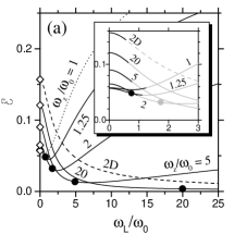
Figure 1: (a) The entanglement measure $\cal E$ of the lowest state with $m=0$ at $R_{W}=1.5$ and various ratios $\omega_{z}/\omega_{0}$ as functions of the parameter $\omega_{L}/\omega_{0}$. The initial (black) parts of the measure (shown in the inset) correspond to the intervals of $\omega_{L}/\omega_{0}$, when the lowest state $m=0$ is the ground state. Full circles denote the values of $\omega_{L}/\omega_{0}$, when the effective 3D confinements become spherically symmetric. (b) The relative strengths of the Coulomb interaction $R_{\mathrm{eff}}^{\mathrm{(2D)}}/R_{W}$ (solid line) and $R_{\mathrm{eff}}^{\mathrm{(1D)}}/R_{W}$ (dash-dotted line) for the lowest state $m=0$ at various ratios $\omega_{z}/\omega_{0}$ as functions of the parameter $\omega_{L}/\omega_{0}$.

At zero magnetic field ($\omega_{L}/\omega_{0}=0$) the entanglement of the lowest state with $m=0$ decreases if the ratio $\omega_{z}/\omega_{0}$ decreases from $\infty$ (2D model) to $1$ (spherically symmetric 3D model); see open symbols (diamonds) in Fig. 1(a). This effect could be explained by introducing the effective charge $k_{\mathrm{eff}}$ ec which determines the effective electron-electron interaction $V_{C}^{\mathrm{eff}}=k_{\mathrm{eff}}/\rho_{12}$ in the QD. In the 3D dot the electrons can avoid each other more efficiently than in the 2D one. Consequently, the Coulomb interaction has a smaller effect when $\omega_{0}\approx\omega_{z}$ (the ratio $k_{\mathrm{eff}}/k\approx 0.5$) than in the anisotropic case $\omega_{0}\ll\omega_{z}$ ($k_{\mathrm{eff}}/k=1$). Therefore, a decreasing of the ratio $\omega_{z}/\omega_{0}$ yields an analogous effect as the reduction of the electron-electron interaction – a weaker mixing of the single-particle states and, consequently, a lowering of the entanglement.

By increasing the magnetic field from zero to $B_{\mathrm{sph}}\sim\omega_{L}^{\mathrm{sph}}=\sqrt{\omega_{z}^{2}-\omega_{0}^{2}}$ (see full circles in Fig. 1(a)) the entanglement decreases. Similar to the case $B=0$, one would expect the decrease of the effective electron-electron interaction with the evolution of the effective confinement from the disk shape ($\Omega<\omega_{z}$) to the spherical form ($\Omega=\omega_{z}$). Further increase of the magnetic field yields the increase of the entanglement. The effective confinement becomes again anisotropic (now with $\Omega>\omega_{z}$). Evidently, for $\omega_{z}/\omega_{0}\to\infty$ (2D model) the minimum of $\cal E$ is shifted to infinity, i.e. in this case the entanglement decreases monotonically with the increase of the field (dashed line in Fig. 1(a)).

The entanglement evolution can be explained by the influence of the magnetic field on the effective strength of the electron-electron interaction, which transforms the Wigner parameter $R_{W}$ to the form $R_{\mathrm{\Omega}}=l_{\Omega}/a^{*}$. The length $l_{\Omega}=\sqrt{\hbar/m^{*}\Omega}$ characterizes the effective lateral confinement.

For the quasi-2D system ($\Omega\ll\omega_{z}$), the influence of magnetic field on the effective strength $R_{\Omega}\Rightarrow R_{\mathrm{eff}}^{\mathrm{(2D)}}=(k_{\mathrm{eff}}^{\mathrm{(2D)}}/l_{\Omega})/\hbar\Omega$ is twofold. Here $k_{\mathrm{eff}}^{\mathrm{(2D)}}=\langle\rho_{12}V_{C}\rangle$ (see Eq. (18)-(20) in Ref. ec ), where $V_{C}=k/r_{12}$ is the full 3D Coulomb interaction. The magnetic field affects the effective confinement $\hbar\Omega$ as well as the effective charge. With the increase of the effective confinement the effective charge $k_{\mathrm{eff}}^{\mathrm{(2D)}}/k\to 1$ and, therefore, the effective stength decreases as $R_{\mathrm{eff}}^{\mathrm{(2D)}}\sim 1/\sqrt{\Omega}$ (see Fig. 1(b)).

For $\Omega\gg\omega_{z}$ (very strong magnetic field) the electrons are pushed laterally towards the dot’s center. The magnetic field, however, does not affect the vertical confinement. As a consequence the electrons practically move only in the z-direction, and the QD becomes a quasi-1D system. In this case the effective strength is $R_{\Omega}\Rightarrow R_{\mathrm{eff}}^{\mathrm{(1D)}}=(k_{\mathrm{eff}}^{\mathrm{(1D)}}/l_{z})/\hbar\omega_{z}$. Here the effective charge $k_{\mathrm{eff}}^{\mathrm{(1D)}}=\langle|z_{12}|V_{C}\rangle$, and $l_{z}=\sqrt{\hbar/m^{*}\omega_{z}}$ is the oscillator length of the vertical confinement. For the lowest state with $m=0$ it can be shown that $k_{\mathrm{eff}}^{\mathrm{(1D)}}/k=(1+\sqrt{\omega_{z}/\Omega})^{-1}$. At a very strong magnetic field the ratio $k_{\mathrm{eff}}^{\mathrm{(1D)}}/k\to 1$ which yields the maximal value $R_{\mathrm{eff}}^{\mathrm{(1D)}}\sim 1/\sqrt{\omega_{z}}$. When $\Omega=\omega_{z}$ the 3D system is far from both the 2D and the 1D limits. As a result, $R_{\mathrm{eff}}^{\mathrm{(2D)}}$ and $R_{\mathrm{eff}}^{\mathrm{(1D)}}$ do not match smoothly (see Fig. 1(b)). However, it is clear that the effective strength reaches the minimum around this point, i.e. when the transition from the lateral to the vertical localization of two electrons takes place.

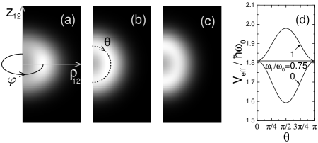
Figure 2: The ground state probability density (the relative motion part, $m=0$) for the near-spherical ($\omega_{z}/\omega_{0}=1.25$) two-electron QD with $R_{W}=1.5$ ($\hbar\omega_{0}=5.627$ meV) and $g^{*}=-0.44$ at different values of the magnetic field: (a) $\omega_{L}/\omega_{0}=0$, (b) $\omega_{L}/\omega_{0}=0.75$, (c) $\omega_{L}/\omega_{0}=1$. For the spherically symmetric case (b) the maximum of the probability density spreads uniformly over the spherical shell of a radius $r_{0}$. The panel (d) displays the potential $V_{\mathrm{eff}}(\rho_{12},z_{12})$ on this sphere ($\rho_{12}=r_{0}\sin\theta$, $z_{12}=r_{0}\cos\theta$) for the cases (a-c).

In order to get a deeper insight into this transition we examine the probability density $|\psi({\bf r}_{12})|^{2}$ for the ground state, when $m=0$. Such a ground state can be realized for a near spherical QD with $\omega_{z}/\omega_{0}=1.25$. For this ratio and $R_{W}=1.5$ the first S-T transition occurs at $\omega_{L}/\omega_{0}\approx 1.11$ (see the inset in Fig. 1(a)). The spherical symmetry ($\Omega=\omega_{z}$) sets up at $\omega_{L}^{\rm sph}/\omega_{0}=0.75$, i.e., in the ground state. For the magnetic field strengths $\omega_{L}<\omega_{L}^{\rm sph}$ ($\Omega<\omega_{z}$) the density maximum forms a ring in the $(x_{12},y_{12})$-plane (a consequence of the axial symmetry). Fig. 2(a) shows the cut of this density with the $(\rho_{12},z_{12})$-plane at arbitrary azimuthal angle $\varphi$. For $\omega_{L}=\omega_{L}^{\rm sph}$ the maximum of the probability density forms a spherical shell (visible if we rotate Fig. 2(b) around $z_{12}$-axis). For $\omega_{L}>\omega_{L}^{\rm sph}$ ($\Omega>\omega_{z}$) two separate density maxima start to grow, located symmetrically in the $z_{12}$-axis (see Fig. 2(c)). In contrast to the corresponding behaviour of the entanglement, a fuzzy transition manifests itself in the probability density for the chosen dot’s parameters. In fact, the entanglement evolution guides us to trace a geometrical crossover from the lateral to the vertical localization of the electrons.

The probability density evolution due to the magnetic field shown in Figs. 2(a-c) can be elucidated by means of the analysis of the effective potential $V_{\mathrm{eff}}=\frac{1}{2}\,\mu\,(\Omega^{2}\rho_{12}^{2}+\omega_{z}^{2}z_{12}^{2})+k/r_{12}+\hbar^{2}m^{2}/(2\mu\rho_{12}^{2})$. Namely, the maxima of the probability density for the ground state are directly related to the minima of $V_{\mathrm{eff}}$. For $\omega_{L}<\omega_{L}^{\rm sph}$ the potential surface has the minimum at $\rho_{12}=\rho_{0}$, $z_{12}=0$, where $\rho_{0}=(k/\mu\Omega^{2})^{1/3}$ if $m=0$. By increasing the magnetic field to values $\omega_{L}>\omega_{L}^{\rm sph}$ this minimum transforms to the saddle point in the $(\rho_{12},z_{12})$-plane, but two new minima divided by this saddle (potential barrier) appear. For $m=0$ these minima are located at $z_{12}=\pm z_{0}$, where $z_{0}=(k/\mu\omega_{z}^{2})^{1/3}$.

For weakly anisotropic (near spherical) systems it is convenient to use the spherical coordinates $(r_{12},\theta,\varphi)$, where the polar angle is $\theta\equiv\arctan(\rho_{12}/z_{12})$. In these coordinates the positions of the minima are $r_{12}=\rho_{0}$, $\theta=\pi/2$ for $\Omega<\omega_{z}$ and $r_{12}=z_{0}$, $\theta=0,\pi$ for $\Omega>\omega_{z}$; see the cases $\omega_{L}/\omega_{0}=0$ and $1$, respectively, in Fig. 2(d). Note, that due to the axial symmetry the azimuthal angle $\varphi$ is arbitrary. The maximum at $\theta=\pi/2$ for $\Omega>\omega_{z}$ (the case $\omega_{L}/\omega_{0}=1$ in Fig. 2(d)) corresponds to the saddle point at $z_{12}=0$. If we consider small oscillations around a minimum, the effective potential can be written in the form $V_{\mathrm{eff}}\approx V_{0}+\frac{1}{2}\,\omega_{1}^{2}\,q_{1}^{2}+\frac{1}{2}\,\omega_{2}^{2}\,q_{2}^{2}$ (the expansion up to the quadratic terms), where $q_{1}=\Delta r$, $q_{2}=r_{0}\Delta\theta$ are the normal coordinates. Here $r_{0}=\rho_{0}$ when $\Omega<\omega_{z}$, whereas $r_{0}=z_{0}$ when $\Omega>\omega_{z}$. The corresponding normal frequencies (if $m=0$) are: (i) $\omega_{1}=\sqrt{3}\,\Omega$, $\omega_{2}=(\omega_{z}^{2}-\Omega^{2})^{1/2}$ for $\Omega<\omega_{z}$; and (ii) $\omega_{1}=\sqrt{3}\,\omega_{z}$, $\omega_{2}=2\,(\Omega^{2}-\omega_{z}^{2})^{1/2}$ for $\Omega>\omega_{z}$. For the spherically symmetric case ($\Omega=\omega_{z}$) one has $\omega_{2}=0$ and the minima of $V_{\mathrm{eff}}$ degenerate to the sphere of radius $r_{0}=\rho_{0}=z_{0}$. In other words, the potential $V_{\mathrm{eff}}$ becomes independent on the angle $\theta$; see the case $\omega_{L}/\omega_{0}=0.75$ in Fig. 2(d). As a consequence, the wave function becomes spherically symmetric (Fig. 2(b)). The quantum oscillations evolve in a way similar to those of quantum phase transitions studied for model systems Sad .

In conclusion, we found that the entanglement of the lowest state with $m=0$ in axially symmetric two-electron QDs, being first a decreasing function of the magnetic field, starts to increase after the transition point $\omega_{L}^{\mathrm{sph}}=\sqrt{\omega_{z}^{2}-\omega_{0}^{2}}$ with the increase of the magnetic field. This behaviour is understood as the transition from the lateral to the vertical localization of two electrons. It is especially noteworthy that the transition point associated with the onset of the spherical symmetry is robust at any strength of the Coulomb interaction at the fixed ratio of the quantum confinement $\omega_{z}/\omega_{0}$. Varying the magnetic field around the transition point, one can control the increase/decrease of the entanglement in QDs. We paid a special attention to the case when the shape transition occurs in the dot’s ground state. This can happen for weakly anisotropic QDs (see the inset in Fig. 1(a)). Note that for a typical ratio $\omega_{z}\gg\omega_{0}$ considered in literature the lowest $m=0$ state becomes an excited state before the shape transition takes place. Therefore, it would be difficult to recognize such type of transitions in previously considered cases. We speculate that the transition may be observed in optical experiments, where the appearance of the wave function in the vertical direction may affect the photoluminescence of the QD. However, this question requires a dedicated study and is beyond the scope of the present paper.

This work is partly supported by RFBR Grant No.11-02-00086 (Russia), Project 171020 of Ministry of Education and Science of Serbia; by the CAIB and FEDER (Spain).

References

- (1) S. Sachdev, Quantum Phase Transitions (Cambridge University Press, Cambridge, 2011) 2nd Edition.
- (2) K. von Klitzing, G. Dorda, and M. Pepper, Phys. Rev. Let. 45, 494 (1980); D. C. Tsui, H. L. Stormer, and A. C. Gossard, ibid, 48, 1559 (1982).
- (3) L. Amico, R. Fazio, A. Osterloh, and V. Vedral, Rev. Mod. Phys. 80, 517 (2008).
- (4) M. Tichy, F. Mintert, and A. Buchleitner, J. Phys. B: At. Mol. Opt. Phys. 44, 192001 (2011).
- (5) S. M. Reimann and M. Manninen, Rev. Mod. Phys. 74, 1283 (2002).
- (6) P. A. Maksym, H. Imamura, G. P. Mallon, H. Aoki, J. Phys. Condens. Matter 12, R299 (2000).
- (7) C. Yannouleas and U. Landman, Rep. Prog. Phys. 70, 2067 (2007).
- (8) S. Kais, D. R. Herschbach, and R. D. Levine, J. Chem. Phys. 91, 7791 (1989); M. Taut, J. Phys. A 27, 1045 (1994); B. S. Kandemir, J. Math. Phys. 46, 032110 (2005); W. Zhu and S.B. Trickey, Phys. Rev. A 72, 022501 (2005).
- (9) R. G. Nazmitdinov, Physics of Particles and Nuclei 40, 71 (2009).
- (10) W. Kohn, Phys. Rev. 123, 1242 (1961).
- (11) V. Fock, Z. Phys. 47, 446 (1928); C. G. Darwin, Proc. Cambridge Philos. Soc. 27, 86 (1930).
- (12) M. Wagner, U. Merkt, and A. V. Chaplik, Phys. Rev. B 45, 1951 (1992).
- (13) R. G. Nazmitdinov and N. S. Simonović, Phys. Rev. B 76, 193306 (2007).
- (14) N. S. Simonović and R. G. Nazmitdinov, Phys. Rev. B 67, 041305(R) (2003).
- (15) A. Wojs, P. Hawrylak, S. Fafard, and L. Jacak, Phys. Rev. B 54, 5604 (1996).
- (16) A. Coleman and V. Yukalov, Reduced Density Matrices (Springer-Verlag, Berlin, 2000).
- (17) J. Naudts and T. Verhulst, Phys. Rev. A 75 062104 (2007); J. P. Coe, A. Sudbery, and I. D’ Amico, Phys. Rev. B 77, 205122 (2008); J. Pipek and I. Nagy, Phys. Rev. A 79, 052501 (2009); R. J Yaez, A. R. Plastino, and J.S. Dehesa, Eur. Phys. J. D 56, 141 (2010); P. Kościk P and A. Okopińska, Phys. Lett. A 374, 3841 (2010).
- (18) Ll. Serra, R. G. Nazmitdinov, and A. Puente, Phys. Rev. B 68, 035341 (2003).
- (19) N. S. Simonović and R. G. Nazmitdinov, Phys. Rev. A 78, 032115 (2008).