Grand-Canonical Quantized Liquid Density-Functional Theory in a Car-Parrinello Implementation

Abstract

Quantized Liquid Density-Functional Theory [Phys. Rev. E 2009, 80, 031603], a method developed to assess the adsorption of gas molecules in porous nanomaterials, is reformulated within the grand canonical ensemble. With the grand potential it is possible to compare directly external and internal thermodynamic quantities. In our new implementation, the grand potential is minimized utilizing the Car-Parrinello approach and gives, in particular for low temperature simulations, a significant computational advantage over the original canonical approaches. The method is validated against original QLDFT, and applied to model potentials and graphite slit pores.

I Introduction

In the recent past, it has been shown that metal-organic frameworks (MOFs) and other molecular framework materials are suitable to adsorb hydrogen in appreciable quantities Rosi et al. (2003) and to separate light-weight fluids, as for example H₂ and D₂.Chen et al. (2008); Teufel et al. (2013); Cai et al. (2012); Liu et al. (2012) At low temperatures, quantum effects of the adsorbed fluids in the rather weak host-guest potential become important, and in the case of quantum sieving they determine the performance of the functional material. Beenakker et al. (1995); Teufel et al. (2013) Quantum effects are also required for the quantitative estimation of the gas adsorption capacity of materials, in particular towards light-weight molecules such as H₂ and D₂.Garberoglio et al. (2005); Kumar et al. (2006) At present, two principal models are established for the treatment of quantum effects: widely spread is the Feynman-Hibbs correction of the classical potential in the Grand Canonical Monte Carlo (GCMC) methodFeynman and Hibbs (1965); Feynman (1975). A more rigorous, albeit computationally more demanding, model is the path integral (PI) technique Feynman (1948); Feynman and Hibbs (1965), that has been applied to describe H₂ and D₂ clusters Chakravarty (1995) and to assess hydrogen adsorption for carbon model pores Wang and Johnson (1999). For a review about the path integral technique we refer to the works of CeperleyCeperley (1995) or Chakravarty.Chakravarty (1997).

In 2005, Patchkovskii et al. suggested to assess the quantum effects of light-weight molecules or atoms, i.e. of hydrogen molecules, within the ideal gas approximation by solving the Schrödinger equation (SE) of a single H₂ particle in the external potential.Patchkovskii et al. (2005) The wave function of the adsorbed hydrogen fluid has been expanded in a plane wave series, and the SE has been solved by explicit diagonalization of the Hamiltonian. In 2007, the numerical implementation has been rigorously revised by using an exponential series to compute the partition function, taking advantage of the sparseness of the Hamiltonian, leading to significant computational advantage for temperatures of 200 K or higher.Patchkovskii and Heine (2007) In order to go beyond the ideal gas treatment, Patchkovskii and Heine applied the Kohn-Sham approach Kohn and Sham (1965) to the problem of a quantum fluid adsorbed in an external potential in the so-called Quantized Liquid Density-Functional Theory (QLDFT).Patchkovskii and Heine (2009) Like in the traditional Kohn-Sham method for electronic systems, the fully interacting system is mapped to a non-interacting system in an effective potential, and the effective one-particle states are occupied within the classical Maxwell-Boltzmann statistics. All terms of the free energy which cannot be expressed explicitly as functional of the density are treated approximately in the excess functional $F_{xc}$, that has been determined such that the experimental isotherms of the uniform fluid served as reference system, similar as the homogeneous electron gas in electronic DFT.

In 2011, Mesa et al. have implemented the proper Bose-Einstein statistics to QLDFT. However, they have shown that even at temperatures of 50 K the classical Maxwell-Boltzmann statistics does not deviate from its rigorous counterpart. On the other hand, quantum effects have been found to be appreciable even at ambient temperature for certain pore sizes.Martinez-Mesa et al. (2011)

The QLDFT method has been successfully applied to describe hydrogen adsorption in carbon foamsMartinez-Mesa et al. (2012), in Porous Aromatic Frameworks (PAFs)Lukose et al. (2012) and to determine the selectivity of $D_{2}$ vs. $H_{2}$ adsorption in the metal-organic framework MFU-4.Teufel et al. (2013)

Today it is generally accepted that reversible hydrogen storage by physisorption in MOFs and other nanoporous materials is only efficient at temperatures that allow cooling with liquid nitrogen (77 K). The presently available QLDFT code Patchkovskii and Heine (2009) shows a rather poor computational performance for temperatures below 100 K. Moreover, it is advantageous to reformulate canonical QLDFT (C-QLDFT) within the grand canonical ensemble to allow a direct comparison to thermodynamic data through the chemical potential, and to be able to compare our simulations with GCMC calculations.

In this article we present the reformulation of QLDFT in the grand-canonical ensemble (GC-QLDFT). For computational efficiency, we suggest a simple approximation of the free energy that is advantageous in particular for low temperature applications. We minimize the grand potential employing the Car-Parrinello (CP) method Car and Parrinello (1985) and compare the performance of this new approach for model potentials and carbon slit pores with C-QLDFT and literature data.

II Method

According to Hohenberg-Kohn and MerminHohenberg and Kohn (1964); Mermin (1965) the exact grand potential $\Omega$ is a functional of the density $\rho(\vec{r})$. This functional can be written as

$$\Omega[\rho]=F_{HKM}[\rho]-\mu\int d^{3}r\,\rho(\vec{r})+\int d^{3}r\,\rho(\vec{r})v_{ext}(\vec{r}).$$ (1)

$F_{HKM}$ denotes the Hohenberg-Kohn and Mermin free energy functional, $\mu$ the chemical potential and $v_{ext}$ is the external potential.

The physical density of a system in contact with a particle reservoir is obtained by fixing the chemical potential and minimizing the functional $\Omega$. The only problem is that the general form of the free energy functional $F_{HKM}$ is unknown and approximations are necessary.

II.1 The QLDFT free energy

In C-QLDFT the free energy $F$ is obtained from the following expression

$$F[\rho]= F_{0}[\rho]-F_{H}[\rho]-\int\,d^{3}r\,v_{xc}(\vec{r})\rho(\vec{r})+F_{xc}[\rho].$$ (2)

$F_{0}$ describes the free energy of a non-interacting system in an effective potential and is discussed below in more detail. $F_{xc}$ denotes the excess functional and $v_{xc}$ is the excess potential which can be obtained by the functional derivative of $F_{xc}$ with respect to the density $\rho$. $F_{H}[\rho]$ is given by

$$F_{H}[\rho]=\frac{1}{2}\int d^{3}r\int d^{3}r^{\prime}\,\rho(\vec{r})v_{12}(|\vec{r}-\vec{r}^{\prime}|)\rho(\vec{r}^{\prime})$$ (3)

where $v_{12}$ denotes the two-body interaction potential between the guest molecules. The choice of $v_{12}$ may range from complete neglection of this typically slightly attractive term to parametrized data from ab initio calculations. For hydrogen adsorption, we have chosen to employ the zero-order term of the extrapolated exact Born-Oppenheimer intermolecular H₂–H₂ interaction potential, as reported by Diep and Johnson.Diep and Johnson (2000) $F_{0}$ is calculated from the non-interacting one-particle partition function $Z_{0}$ using

$$F_{0}=-\frac{N}{\beta}ln\,\frac{Z_{0}}{N}.$$ (4)

$Z_{0}$ is given by a power series expansion of the non-interacting effective Hamiltonian $\mathbf{H_{0}}$

$$\mathbf{H_{0}}= -\frac{\vec{\nabla}^{2}}{2m}+v_{ext}(\vec{r})+\int d^{3}r^{\prime}\,v_{12}(|\vec{r}-\vec{r}^{\prime}|)\rho(\vec{r}^{\prime})+v_{xc}(\vec{r})$$ (5)

of $N$ particles in the external host–guest potential $v_{ext}$:

$$Z_{0}=\mbox{Tr}\,\exp(-\beta\mathbf{H_{0}})\exp(-\beta\mathbf{H_{0}})\approx\mathbf{1}+\sum_{n=1}^{n_{max}}\frac{1}{n!}(\mathbf{-\beta H_{0}})^{n}.$$ (6)

with $\beta=(k_{B}T)^{-1}$. The numerical effort to treat the power series depends on the temperature. In case of high temperatures convergence is rapidly achieved for small numbers of $n_{max}$, but for low temperatures, i.e. at 77 K, convergence requires the inclusion of a large number of terms. Therefore, a simplification to avoid the power series is appreciated and will be suggested below. The power series was originally introduced because of the mapping of an interacting system onto a system of non-interacting particles in an effective potential. In principle, this mapping is very useful because one can obtain a very good approximation of the free energy. It also yields one-particle wave functions in that formalism, and the explicit implementation of the Bose-Einstein statistics is straight-forward.Martinez-Mesa et al. (2011) However, for lower temperatures this approach becomes computationally prohibitively expensive and therefore requires revision.

II.2 The GC-QLDFT grand potential

The C-QLDFT free energy functional will be reformulated in this subsection, avoiding the power series that has marked the computational bottleneck in C-QLDFT. We will obtain the GC-QLDFT grand potential which is based on the minimum principle. The free energy of the effective one-particle reference system $F_{0}$ can be written as follows

$$F_{0}[\rho] =-\frac{N}{\beta}ln\,\frac{Z_{0}}{N}=-\frac{N}{\beta}\left(ln\,Z_{0}-ln\,N\right)$$ (7)

$$=N\left(\sum_{i}f_{i}\int d^{3}r\varphi_{i}(\vec{r})^{*}\mathbf{H_{0}}\varphi_{i}(\vec{r})+\frac{1}{\beta}\sum_{i}f_{i}\log(f_{i})\right)+\frac{N}{\beta}ln\,N.$$

$\varphi_{i}(\vec{r})$ are eigenfunctions of the effective Hamiltonian $\mathbf{H_{0}}$ and $f_{i}$ can be obtained from the eigenvalues by using $Z_{0}^{-1}\exp[-\beta\varepsilon_{i}]$. In C-QLDFT the density $\rho(\vec{r})$ is calculated by rescaling the non-interacting density matrix

$$\gamma_{0}(\vec{r},\vec{r}^{\prime})=\sum_{i}\varphi_{i}(\vec{r})^{*}f_{i}\varphi_{i}(\vec{r}),$$ (8)

yielding a fluid density

$$\rho(\vec{r})=N\gamma_{0}(\vec{r},\vec{r}).$$ (9)

We insert the definition of the Hamiltonian $\mathbf{H_{0}}$ given in equation 5 into 7. By using equation 2 and some simplifications we can write the grand potential in the minimum with $n_{i}:=Nf_{i}$ in the following way

$$\Omega_{0} =\min_{n_{i},\varphi_{i}}\Big{[}\sum_{i}n_{i}\int d^{3}r\,\varphi_{i}(\vec{r})^{*}\Big{(}-\frac{\vec{\nabla}^{2}}{2m}\Big{)}\varphi_{i}(\vec{r})$$ (10)

$$+\int d^{3}r\,\rho(\vec{r})v_{ext}(\vec{r})+\frac{1}{\beta}\sum_{i}n_{i}\log(n_{i})$$

$$+F_{H}[\rho]+F_{xc}[\rho]-\mu\int d^{3}r\,\rho(\vec{r})$$

$$+\sum_{i,j}\lambda_{i,j}\left(\int d^{3}r\varphi_{i}^{*}(\vec{r})\varphi_{j}(\vec{r})-\delta_{i,j}\right)\Big{]}.$$

$\lambda_{i,j}$ are Lagrange multipliers which were introduced to keep the orthogonality of the set of eigenfunctions $\varphi_{i}$.

II.3 The zero-temperature reference system

To simplify equation 10 we apply the zero-temperature approximation to the one particle system, but keep the finite temperature in the many particle system. Such a reference system would be inappropriate if we would describe electrons, since the electron-electron interaction is quite soft and therefore the spin statistics is important in establishing the pair-correlation function. But in case of molecules the intermolecular interaction gets very hard at short distances and completely overwhelms the spin statistics in the pair-correlation function. The work of Mesa et al. Martinez-Mesa et al. (2011) has already shown that Maxwell-Boltzmann and Bose-Einstein statistics are equivalent even for temperatures as low as 50 K.

As the zero temperature reference system appears to be a rather strong approximation we have carefully validated it, and we will show that it yields density profiles in excellent agreement with the C-QLDFT method.

For the zero-temperature approximation and a real wave function we obtain the following expression for the free energy

$$F[\rho] =-\int d^{3}r\phi(\vec{r})\frac{\vec{\nabla}^{2}}{2m}\phi(\vec{r})+F_{H}[\rho]+F_{xc}[\rho]+\int d^{3}r\,\rho(\vec{r})v_{ext}(\vec{r}).$$ (11)

Here we have defined $\phi(\vec{r}):=\sqrt{N}\varphi_{0}(\vec{r})$. Note that with such choice of the free energy the grand potential $\Omega$ can be minimized without any constraint.

Different suggestions for the choice of $F_{xc}$ have already been discussed in ref. Patchkovskii and Heine (2009). There, the most sophisticated functional is the LIE1 (LIE=local interaction expression) excess functional which uses the weighted local density approximation (WLDA) Curtin and Ashcroft (1985). This functional is based on the parametrized thermodynamic data summarized by McCarty et al.McCarty et al. (1981) and based on the experiment of Mills et al .Mills et al. (1977). A double counting term is subtracted. $F^{LIE1}[\rho]$ is given by

$$F^{LIE1}[\rho]=\int d^{3}r\,\rho(\vec{r})\Big{\{}f_{exp}[\rho(\vec{r})]+\beta^{-1}\log\big{(}\frac{Z_{kin}}{\overline{\rho}(\vec{r})V}\big{)}-\frac{1}{2}\rho(\vec{r})\int d^{3}r^{\prime}v_{12}(\vec{r}^{\prime})\Big{\}},$$ (12)

where $Z_{kin}$ is the kinetic partition function obtained from the cyclic-Hamiltonian limit. $f_{exp}$ denotes the free energy per particle obtained in experiment and the weighted density is given by

$$\overline{\rho}(\vec{r})=\int d^{3}r^{\prime}w(|\vec{r}-\vec{r}^{\prime}|)\rho(\vec{r}^{\prime}).$$ (13)

$Z_{kin}$, $\overline{\rho}$ and $f_{exp}$ are utilized in exactly the same way as in C-QLDFT and for details we refer to ref. Patchkovskii and Heine (2009). We recognized that $F_{xc}$ cannot simply be replaced by $F_{xc}^{LIE1}$ as the zero temperature approximation is applied to the one-particle system. This approximation affects the kinetic energy of the effective one particle system. The kinetic part of the double counting term (the term $\beta^{-1}\log\big{(}\frac{Z_{kin}}{\overline{\rho}(\vec{r})V}\big{)}$) is in principle not necessary in case of the zero temperature approximation but it controls the density oscillations within the WDA and can therefore not be omitted. For systems involving appreciable density oscillations we found that

$$F_{xc}=F_{xc}^{LIE1}-\beta^{-1}\int d^{3}r\,\rho(\vec{r})\log\left(\frac{Z_{kin}}{\rho(\vec{r})V}\right)$$ (14)

yields satisfactory density profiles for the model systems we have studied. We will call this functional qLIE1 functional (quantum LIE1).

II.4 Approximation of $F_{HKM}$

With the formalism suggested in this work it is possible to approximate the Hohenberg-Kohn and Mermin free energy $F_{HKM}$ similar to the strategy used in classical liquid density functional theory (CLDFT) Saam and Ebner (1977); Evans (1979); Singh (1991).

The most straight-forward approximation of the free energy for the confined fluid is the free energy of the uniform fluid of the same density, which means

$$F_{HKM}[\rho]\approx\int d^{3}r\,\rho(\vec{r})f_{exp}[\rho(\vec{r})].$$ (15)

This is the local density approximation (LDA), well-known in electronic DFT, but in our case for the Hohenberg-Kohn and Mermin free energy functional. It should be noted that the LDA functional goes beyond the CLDFT strategy because it is exact in the uniform fluid limit. To go beyond the LDA, we employ the weighted local density approximation (WLDA)

$$F_{HKM}[\rho] \approx-\frac{1}{\beta}\int d^{3}r\,\rho(\vec{r})\log\left(\frac{Z_{kin}}{\rho(\vec{r})V}\right)+F_{H}[\rho]+F_{xc}^{LIE-1}[\rho,\overline{\rho}].$$ (16)

The first two terms in equation 16 were chosen in order to fulfil the uniform fluid limit exactly. We will call this functional cLIE1 functional (classical LIE1), because we will see that it only reflects the classical LIE1 limit. The approximations 15, 16 and 11 (in connection with equation 14) were implemented into a new software that allows the minimization of the grand potential. The software is published at our website http://www.jacobs-university.de/ses/theine/research. Other functional choices are definitely possible and we plan to evaluate more sophisticated approximations than LDA, cLIE1 or qLIE1.

II.5 Grand canonical ensemble and external pressure

The choice of the ensemble should not influence the result in the thermodynamic limit. From that point of view it does not matter if the method is formulated in the canonical or grand canonical ensemble. But the standard methods like GCMC or PI-GCMCWang et al. (1997) typically use the grand canonical ensemble, and thus this choice is more convenient to directly compare the QLDFT results with other theoretical approaches. In the grand canonical ensemble the external pressure and the chemical potential can be related to each other directly. This can be achieved most conveniently by using the available data from experiments for the uniform fluid.

It is straight-forward to obtain the free energy of the uniform fluid from experiment over a wide range of pressures and temperatures Patchkovskii and Heine (2009), and also the molar volume is available. This information is sufficient to relate the chemical potential, pressure and temperature using standard thermodynamic relations.

For a given input pressure and temperature we can calculate the free energy $F_{N}$ per $N$ particles and the molar volume $V_{N}$ from experiment. Thus, we obtain the grand potential $\Omega_{N}$ per mole from $\Omega_{N}=-pV_{N}$. The chemical potential is given by

$$\mu=\frac{F_{N}-\Omega_{N}}{N}$$ (17)

II.6 Minimization within the Car-Parrinello scheme

For the minimization of the grand potential $\Omega$ we have chosen the Car-Parrinello (CP) scheme Car and Parrinello (1985). This scheme was originally introduced to allow molecular dynamics simulations based on first principles forces on the atoms. However, this scheme can be used to minimize any functional. The CP method is often discussed in the literature (for an overview about the basic techniques see for example ref. Tuckerman and Parrinello (1994)), and we only show the main equations here. First, we discuss the minimization of an approximation of the grand potential $\Omega$. A grid is covering the space in the simulation box. We denote a grid point with $R$, for the corresponding density at this point we use $\rho_{R}$ and for the wave function $\phi_{R}$. In case of the grand canonical ensemble we do not have to fix the number of particles, but we have to take care that the density at a grid point $R$ cannot be negative. This constraint is already fulfilled because $\rho_{R}$ is given by the square of the non-normalized wave function $\phi_{R}$, which means $\rho_{R}:=\phi_{R}^{2}$.

Similar to Car and Parrinello we introduce a fictitious kinetic energy term for $\phi_{R}$. The Lagrange function is given by

$$\mathcal{L}=\frac{m_{x}}{2}\sum_{R}\,\dot{\phi}_{R}^{2}-\Omega[{\phi_{R}}]$$ (18)

where $m_{x}$ is the fictitious mass parameter. Using the Euler-Lagrange equations we obtain

$$m_{x}\ddot{\phi}_{R}=-\frac{\partial\Omega}{\partial\phi_{R}}-m_{x}\alpha\dot{x}_{R}.$$ (19)

Here we have added a friction term $-m_{x}\alpha\dot{\phi}_{R}$ with friction parameter $\alpha$. The set of the differential equations can be discretized using the Verlet algorithm Verlet (1967, 1968), where the time derivatives $\dot{\phi}_{R}$ and $\ddot{\phi}_{R}$ are replaced by

$$\dot{\phi}_{R}\approx\frac{\phi_{R}(+)-\phi_{R}(-)}{2\Delta}$$ (20)

and

$$\ddot{\phi}_{R}\approx\frac{\phi_{R}(+)-2\phi_{R}(0)+\phi_{R}(-)}{\Delta^{2}},$$ (21)

respectively. $(0)$ denotes the present, $(+)$ the next and $(-)$ the previous iteration, differing by time step $\Delta$. We can easily rearrange the terms to obtain $\phi_{R}$ for the next step

$$\phi_{R}(+) =\left(1+\frac{m_{x}\alpha}{2\Delta}\right)^{-1}$$ (22)

$$\times\left[-\frac{\Delta^{2}}{m}\frac{\partial\Omega}{\partial\phi_{R}}+2\phi_{R}(0)-(1-\frac{m_{x}\alpha}{2\Delta})\phi_{R}(-)\right].$$

Note that an explicit calculation of constraints is not necessary in the suggested formalism. Choosing a reasonable time step $\Delta$ and friction parameter $\alpha$, the scheme yields the minimum of the functional $\Omega$. From now on we will call this treatment the CP-GC-QLDFT method.

III Benchmark Applications

To test the presented method we applied it to the adsorption of molecular hydrogen in three selected well known systems that have been studied intensively in the literature. The first one is the hard-wall slit pore model potential, the second density fluctuations around a fixed hydrogen probe potential and the third one the graphite slit pore with variable pore size. Further applications employing CP-GC-QLDFT to MOFs are currently in progress.

III.1 Model systems

The hard-wall slit pore has been widely studied in the literature (see for example Hansen and McDonald (2006)) and can safely be regarded as the benchmark system for the adsorption of molecular hydrogen. The particle-in-a-box character of the boundary implies strong fluctuations of the hydrogen density and thus marks a challenge for the numerical approach. The strong oscillations of the density cannot be described well within the LDA. However, satisfactory results can be obtained employing the WLDA, as already shown earlier.Patchkovskii and Heine (2009) We use these systems to test our CP-GC-QLDFT method thoroughly: We benchmark the results by comparing the hydrogen density profiles to those obtained with the C-QLDFT method, and we evaluate the computational performance in terms of convergence and computer time.

The central potential describes a fixed hydrogen molecule at the center of the unit cell. This model allows us to study the density oscillations of the quantum liquid associated to the ‘first solvation shell’ around a fixed fictitious hydrogen molecule.

The convergence of the CP-GC-QLDFT method is illustrated in Figure 1 for an exemplary slit pore. We have used a temperature of 100 K and a pressure of 1 kbar, and employed the cLIE1 functional. The size of the unit cell was chosen to be $a=b=5$Åand $c=20$Å. A grid of 1 point per Åin $x$ and $y$ direction and 10 points per Åin $z$ direction was applied. As shown in Figure 1, after approximately 400 simulation steps (we use $\Delta=0.05$ for the presented example) the change in the grand potential becomes negligible. After $\sim$ 200 steps the number of particles in the unit cell changes by $\Delta N=10^{-2}$ particles, after $\sim$ 300 steps by $\Delta N=10^{-4}$. We consider the system to be converged by $\Delta N=10^{-5}$ which is obtained after $\sim$ 400 steps.

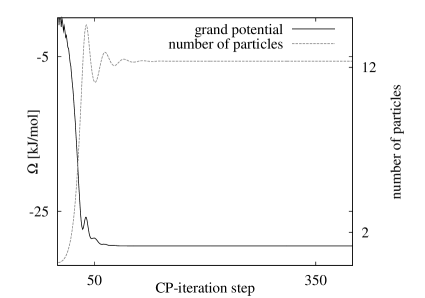
Figure 1: Grand potential $\Omega$ (left $y$-axis) in dependence of the simulation step. The grand potential and the number of particles (right $y$-axis) show convergence after 400 steps (the time step was chosen to be $\Delta=0.05$) for the presented example. The calculation refers to a hard-wall slit pore at $T=$100 K and $p$=1 kbar.

It is not straight-forward to compare the grand canonical and the canonical ensemble: While in C-QLDFT the number of particles in the simulation box is fixed, in GC-QLDFT we fix the external pressure or, equivalently, the chemical potential. In order to achieve the best possible comparison, we have first converged the system in the CP-GC-QLDFT approach, and then used the obtained molar volume as input variable for C-QLDFT. Calculations have been carried out for $T$=100 K, 200 K and 300 K. In case of CP-GC-QLDFT we have applied the LDA, cLIE1 and qLIE1 functionals in case of C-QLDFT the LIE0 (for details see Patchkovskii and Heine (2009)) and LIE1 functionals. Calculations have been carried out for the same setup and temperatures as reported above.

In Figure 2 the density profiles of both methods are compared for the central potential. As expected, within the LDA we obtain a nearly shapeless density profile. The LDA, where the $v_{12}$ intermolecular potential is incorporated in the HKM operator, and LIE0, that is LDA with neglection of the interparticle interactions of the fluid, give - not surprisingly - very similar results.

The non-physical absence of the density oscillations has already been discussed in detail earlier.Patchkovskii and Heine (2009) Here, we note that it is irrelevant if the local approximation is made to the classical or the quantum-mechanical system and state that it should only be applied if the potential variation and the associated density oscillations are expected to be very small.

Because of the fact that the magnitude of the density oscillations is controlled by the choice of the weighting function $w$ used to construct $\overline{\rho}$, we are not surprised that the densities of the cLIE1, qLIE1 and the LIE-1 functionals are in rather close agreement with each other.

The classical LIE1 functional produces a discontinuity of the density profile for the hard wall potential (see figure 3). This behaviour is due to the discontinuous character of the model potential and thus will not occur when treating real systems with parametrized force fields describing the host-guest interaction.

In contrast to the classical functional (cLIE1), the qLIE1 correctly describes the density oscillations and also the quantum behaviour in a satisfactory manner: in comparison to the C-QLDFT result, small differences in the density profile are observed close to the hard walls. We observe a slight overdelocalization in qLIE1 due to the choice of the zero temperature reference system, a consequence of the missing higher-energy one-particle states.

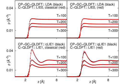
Figure 2: Density profiles of the hydrogen quantum liquid in the central potential obtained with the C-QLDFT and CP-GC-QLDFT methods. A pressure of 1 kbar was chosen for the CP-GC-QLDFT calculations. On the left-hand side it is shown that the cLIE1 (LDA) density profile is nearly the same compared to the classical C-QLDFT LIE1 (LIE0) result. On the right-hand panel we compare the LDA and qLIE1 density profiles with the results obtained from non-classical LIE0 and LIE1 calculations.

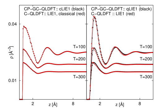
Figure 3: Density profiles of the hydrogen quantum liquid for the hard-wall potential. The position of the hard wall is $z=0.5$ Å  for the presented example. The CP-GC-QLDFT result ($p$=1 kbar) obtained with the cLIE1 functional (left-hand side) shows a discontinuity at the hard wall in contrast to the result obtained with qLIE1 (right-hand side). The LDA result for the hard-wall potential is not presented. In that case one obtains a step-like density profile without a quantum correction close to the hard wall.

In contrast to the cLIE1 approximation, the qLIE1 functional is able to describe the density oscillations and also the quantum behaviour in a satisfactory manner. In comparison to the C-QLDFT result, small differences in the density profile can be observed close to the hard walls. The zero temperature reference system delocalizes the particles a bit too much which is a consequence of the missing higher-energy one-particle states. The differences have, however, only numerical character and if necessary one can change the weighting function used in the qLIE1 functional to obtain a better agreement. In future we plan to analyse this behaviour in more detail by comparing our results with PI calculations.

At this point we compare the computational performance of C-QLDFT with CP-GC-QLDFT. A big advantage of the CP-GC-QLDFT treatment is that the method is formulated in a way that the speed of the calculations does not depend strongly on the temperature. In the exponential series employed to calculate the partition function in C-QLDFTPatchkovskii and Heine (2007), low temperatures result in non-sparse Hamiltonians and long series are necessary to reach convergence. In our direct minimization scheme there is no explicit dependency on the temperature, and hence this scheme works with about the same performance for all temperatures tested. It should be noted that for a calculation with $T$=50 K the computer time on the same machine accounts for a few seconds for the CP-GC-QLDFT scheme, compared to more than a week using the C-QLDFT scheme, employing the exponential series. For high temperatures (e.g. 300 K) both codes show comparable performance.

III.2 Carbon layers

Experiments in the late 1990s have reported that porous carbon structures can store a significant amount of hydrogen even at room temperature Dillon et al. (1997); Chambers et al. (1998). These experiments have motivated a lot of theoretical and experimental investigations of carbon based materials in the last decades. Today it is known that these experiments were not reproducible and the hydrogen uptake of these materials is only significant at much lower temperatures. However, carbon based materials are still among the attractive candidates for hydrogen storage. For reviews about that topic we refer to Hirscher et al. (2009); Meregalli and Parrinello (2001).

For our benchmark applications we will focus on graphite slit pores (GSPs). GSPs have been studied theoretically with GCMC calculations by Aga et al. Aga et al. (2007) and Rzepka et al. Rzepka et al. (1998), with the PI-GCMC method Wang et al. (1997) by Wang and Johnson Wang and Johnson (1999) (idealized carbon slit pore) and also with a free energy based method by Patchkovskii et al. Patchkovskii et al. (2005). Today it is well known that a change of the graphite interlayer distance influences the hydrogen uptake significantly, depending on external pressure and temperature.

For the theoretical treatment of GSPs, different $C-H_{2}$ potentials have been employed in the past. Wang et al. Wang et al. (1980) suggested a Lennard-Jones potential (LJ)

$$V(r)=4\varepsilon\left[\left(\frac{\sigma}{r}\right)^{12}-\left(\frac{\sigma}{r}\right)^{6}\right]$$ (23)

with $\sigma$ = 2.97 Å and $\varepsilon$ = 3.69 meV, while Patchkovskii et al. Patchkovskii et al. (2005) have chosen a Buckingham potential (B)

$$V(r)=Ae^{-\alpha r}+C_{6}r^{-6}$$ (24)

with $A$=1099.52 eV, $\alpha$ = 3.5763 Å^-1 and $C_{6}$ = -17.36 eV Å⁶. It was already discussed that the B potential predicts a significantly stronger $C-H_{2}$ binding energy than the LJ potential with the parameters reported above, and therefore predicts a larger amount of hydrogen uptake.Aga et al. (2007)

It should be mentioned that the PI-GCMC calculations of Wang and Johnson Wang and Johnson (1999) were performed with the Crowell-Brown (CB) potential Crowell and Brown (1982). This potential depends on the number and distance of graphene planes. As we wanted to apply potentials which can be used in a more general way for further applications, we decided to focus on the LJ and B potentials only.

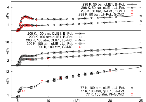
Figure 4: Weight percent adsorption in dependence of the interlayer distance $d$. Results for $T$=298 K at $p$=50 bar, as well as for $T$=77 K and 200 K at $p$=101.325 bar are shown. The results are compared with GCMC calculations of Aga and co-workers Aga et al. (2007) ($T$=300 K), with the GCMC results of Rzepka et al. Rzepka et al. (1998) ($T$=200 K) and with the PI-GCMC calculations of Wang and Johnson Wang and Johnson (1999).

The size of the GSP unit cell was chosen to be $a$ = 12.30622099 Å, $b$ = 12.789 Åand $c$ = 4$d$. $d$ denotes the distance between the graphene layers. We used 6 grid points per Åfor our calculations. The gravimetric adsorption capacity (in weight percent wt %) is shown in Figure 4. Simulations have been carried out at $T$=77 K, 200 K and 298 K. In case of 77 K and 200 K we applied $p$= 101.325 bar, in case of $T$=298 K $p$=50 bar. In all cases, the chosen force field has an enormous influence on the predicted hydrogen storage capacity. It illustrates the importance of high precision host-guest interaction potentials. Our CP-GC-QLDFT results with cLIE1 functional match Aga et al.’s GCMC calculations Aga et al. (2007) very closely at room temperature. We observe the same maximum between 6.2 and 6.6 Å, caused by the superposition of the host-guest interaction of upper and lower layer. Like GCMC, CP-GC-QLDFT also predicts a vanishing hydrogen density at approximatly 5 Å.

The qLIE1 functional predicts a smaller hydrogen uptake for both potentials. This can be expected because quantum effects lower the heat of adsorption. Our results match the GCMC calculations of Rzepka et al. Rzepka et al. (1998) and the PI-GCMC calculations of Wang and Johnson Wang and Johnson (1999) closely. We assume that different potentials and the rather different numerical implementation explain the deviations.

For the low-temperature and high pressure simulation we have applied the LIE1 functional in the classical (cLIE1) and quantum-mechanical (qLIE1) variants. In case of $T$=77 K we focus on the LJ-potential. We have also done calculations with the B-potential, but our simulations yield results outside the safety range of the available experimental data that is used to determine $F_{xc}$. This is not a problem of the presented method, and should be solved by implementing more accurate experimental data.

The density profiles obtained with the cLIE1 and qLIE1 functionals at $T$=77 K and $p$= 101.325 bar are shown in figure 5. For both functionals we find spherical (disc-like) areas where a large amount of hydrogen is predicted. These high-density areas are a consequence of the external potential which shows the same pattern, as already observed earlier.Patchkovskii et al. (2005)

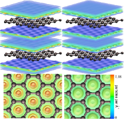
Figure 5: Density profiles for $T$=77 K and $p$= 101.325 bar obtained from CP-GC-QLDFT calculations using the LJ potential. The distance of the graphene layers is 10 Å. On the left-hand side the cLIE1 result is shown, on the right side the qLIE1 result.

IV Conclusions

We have reformulated Quantized Liquid Density-Functional Theory in the grand canonical ensemble. The method has been implemented employing a Car-Parrinello scheme for direct minimization of the grand potential. We obtain a significant computational performance for low-temperature applications. We have compared our implementation with the canonical version of QLDFT for model slit pores and with GCMC calculations for graphite slit pores. In future work we plan to examine more sophisticated approximations of the free energy functional. The software used for this work is available on our website at http://www.jacobs-university.de/ses/theine/research.

V Acknowledgements

Financial support by Deutsche Forschungsgemeinschaft (HE 3543/7-2) within Priority Program SPP1613 is gratefully acknowledged. We thank Prof. Charusita Chakravarty for inspiring discussions.

References

- Rosi et al. (2003) Rosi, N.; Eckert, J.; Eddaoudi, M.; Vodak, D.; Kim, J.; O’Keeffe, M.; Yaghi, O. Science 2003, 300, 1127–1129.
- Chen et al. (2008) Chen, B.; Zhao, X.; Putkham, A.; Hong, K.; Lobkovsky, E. B.; Hurtado, E. J.; Fletcher, A. J.; Thomas, K. M. Journal of the American Chemical Society 2008, 130, 6411–6423, PMID: 18435535.
- Teufel et al. (2013) Teufel, J.; Oh, H.; Hirscher, M.; Wahiduzzaman, M.; Zhechkov, L.; Kuc, A.; Heine, T.; Denysenko, D.; Volkmer, D. Advanced Materials 2013, 25, 635–639.
- Cai et al. (2012) Cai, J.; Xing, Y.; Zhao, X. RSC Advances 2012, 2, 8579–8586.
- Liu et al. (2012) Liu, D.; Wang, W.; Mi, J.; Zhong, C.; Yang, Q.; D, W. Industrial and Engineering Chemistry Research 2012, 51, 434–442.
- Beenakker et al. (1995) Beenakker, J. J. M.; Borman, V. D.; Krylov, S. Y. Chem. Phys. Lett. 1995, 232, 379–382.
- Garberoglio et al. (2005) Garberoglio, G.; Skoulidas, A. I.; Johnson, J. K. The Journal of Physical Chemistry B 2005, 109, 13094–13103, PMID: 16852629.
- Kumar et al. (2006) Kumar, A. V. A.; Jobic, H.; Bhatia, S. K. The Journal of Physical Chemistry B 2006, 110, 16666–16671, PMID: 16913804.
- Feynman and Hibbs (1965) Feynman, R. P.; Hibbs, A. R. Quantum Mechanics and Path Integrals; New York: McGraw-Hill, 1965.
- Feynman (1975) Feynman, R. P. Statistical Mechanics; Benjamin: New-York, 1975.
- Feynman (1948) Feynman, R. P. Rev. Mod. Phys. 1948, 20, 367–387.
- Chakravarty (1995) Chakravarty, C. Molecular Physics 1995, 84, 845–852.
- Wang and Johnson (1999) Wang, Q.; Johnson, J. K. The Journal of Chemical Physics 1999, 110, 577–586.
- Ceperley (1995) Ceperley, D. Reviews of Modern Physics 1995, 67, 279.
- Chakravarty (1997) Chakravarty, C. International reviews in physical chemistry 1997, 16, 421–444.
- Patchkovskii et al. (2005) Patchkovskii, S.; Tse, J. S.; Yurchenko, S. N.; Zhechkov, L.; Heine, T.; Seifert, G. Proceedings of the National Academy of Sciences of the United States of America 2005, 102, 10439–10444.
- Patchkovskii and Heine (2007) Patchkovskii, S.; Heine, T. Phys. Chem. Chem. Phys. 2007, 9, 2697–2705.
- Kohn and Sham (1965) Kohn, W.; Sham, L. Physical Review 1965, 140, 1–5.
- Patchkovskii and Heine (2009) Patchkovskii, S.; Heine, T. Phys. Rev. E 2009, 80, 031603.
- Martinez-Mesa et al. (2011) Martinez-Mesa, A.; Yurchenko, S. N.; Patchkovskii, S.; Heine, T.; Seifert, G. The Journal of Chemical Physics 2011, 135, 214701.
- Martinez-Mesa et al. (2012) Martinez-Mesa, A.; Zhechkov, L.; Yurchenko, S. N.; Heine, T.; Seifert, G.; Rubayo-Soneira, J. The Journal of Physical Chemistry C 2012, 116, 19543–19553.
- Lukose et al. (2012) Lukose, B.; Wahiduzzaman, M.; Kuc, A.; Heine, T. The Journal of Physical Chemistry C 2012, 116, 22878–22884.
- Car and Parrinello (1985) Car, R.; Parrinello, M. Phys. Rev. Lett. 1985, 55, 2471–2474.
- Hohenberg and Kohn (1964) Hohenberg, P.; Kohn, W. Phys. Rev. 1964, 136, B864–B871.
- Mermin (1965) Mermin, N. D. Phys. Rev. 1965, 137, A1441–A1443.
- Diep and Johnson (2000) Diep, P.; Johnson, J. K. The Journal of Chemical Physics 2000, 112, 4465.
- Curtin and Ashcroft (1985) Curtin, W. A.; Ashcroft, N. W. Phys. Rev. A 1985, 32, 2909–2919.
- McCarty et al. (1981) McCarty, R. D.; Hord, J.; Roder, H. M. Selected properties of hydrogen (engineering design data); Technical Report, 1981.
- Mills et al. (1977) Mills, R.; Liebenberg, D.; Bronson, J.; Schmidt, L. The Journal of Chemical Physics 1977, 66, 3076.
- Saam and Ebner (1977) Saam, W.; Ebner, C. Physical Review A 1977, 15, 2566–2568.
- Evans (1979) Evans, R. Advances in Physics 1979, 28, 143–200.
- Singh (1991) Singh, Y. Physics Reports 1991, 207, 351–444.
- Wang et al. (1997) Wang, Q.; Johnson, J. K.; Broughton, J. Q. The Journal of Chemical Physics 1997, 107, 5108–5117.
- Tuckerman and Parrinello (1994) Tuckerman, M. E.; Parrinello, M. The Journal of Chemical Physics 1994, 101, 1302–1315.
- Verlet (1967) Verlet, L. Phys. Rev. 1967, 159, 98–103.
- Verlet (1968) Verlet, L. Phys. Rev. 1968, 165, 201–214.
- Hansen and McDonald (2006) Hansen, J.; McDonald, I. Theory of simple liquids; Academic press, 2006.
- Dillon et al. (1997) Dillon, A. C.; Jones, K. M.; Bekkedahl, T. A.; Kiang, C. H.; Bethune, D. S.; Heben, M. J. Nature 1997, 386, 377–379.
- Chambers et al. (1998) Chambers, A.; Park, C.; Baker, R. T. K.; Rodriguez, N. M. The Journal of Physical Chemistry B 1998, 102, 4253–4256.
- Hirscher et al. (2009) Hirscher, M.; Züttel, A.; Borgschulte, A.; Schlapbach, L. Ceramic Transactions 2009, 202, year.
- Meregalli and Parrinello (2001) Meregalli, V.; Parrinello, M. Applied Physics A: Materials Science & Processing 2001, 72, 143–146.
- Aga et al. (2007) Aga, R. S.; Fu, C. L.; Krčmar, M.; Morris, J. R. Phys. Rev. B 2007, 76, 165404.
- Rzepka et al. (1998) Rzepka, M.; Lamp, P.; De La Casa-Lillo, M. The Journal of Physical Chemistry B 1998, 102, 10894–10898.
- Wang et al. (1980) Wang, S.; Senbetu, L.; Woo, C.-W. Journal of Low Temperature Physics 1980, 41, 611–628.
- Crowell and Brown (1982) Crowell, A.; Brown, J. Surface Science 1982, 123, 296–304.