Permutation complexity of interacting dynamical systems

Abstract

The coupling complexity index is an information measure introduced within the framework of ordinal symbolic dynamics. This index is used to characterize the complexity of the relationship between dynamical system components. In this work, we clarify the meaning of the coupling complexity by discussing in detail some cases leading to extreme values, and present examples using synthetic data to describe its properties. We also generalize the coupling complexity index to the multivariate case and derive a number of important properties by exploiting the structure of the symmetric group. The applicability of this index to the multivariate case is demonstrated with a real-world data example. Finally, we define the coupling complexity rate of random and deterministic time series. Some formal results about the multivariate coupling complexity index have been collected in an Appendix.

1 Introduction

The characterization of complex dynamical systems is a relevant topic arising in different fields of research. This kind of systems are often composed of a large number of interacting components, thus the dynamical behavior may depend on many degrees of freedom. Complex systems display a variety of interesting phenomena, e.g. synchronization Glass2001 and spatially structured collective behavior Tononi1998 ; Strogatz2005 , whose study requires elaborated methods. Recently, ordinal time series analysis has received much attention because its tools present some advantages like robustness against noise and computational efficiency. Ordinal time series analysis is a particular form of symbolic analysis whose ‘symbols’ are ordinal patterns of a given length $L\geq 2$. This concept was introduced by C. Bandt and B. Pompe in their seminal paper Bandt2002 , in which they also introduced permutation entropy as a complexity measure of time series. Since then, ordinal time series analysis has found a number of interesting applications in biomedical sciences, physics, engineering, finance, statistics, etc.

Within the framework of ordinal symbolic dynamics, transcripts arise when considering the relationship between coupled time series. Transcripts are essentially ordinal patterns whose definition exploits the structure of the permutation group. They were introduced in Monetti2009 and applied to characterize the synchronization behavior of two coupled, chaotic oscillators. This work was continued in Amigo2012 , where a general concept of “coupling complexity” was given along with two complexity indices, $C_{1}$ and $C_{2}$, for its quantification. Coupling complexity refers to the relationship among dynamical system components; in general, it differs from the complexity of the individual components or from their sum.

In this paper we approach some basic properties of the complexity index $C_{1}$ (which will be denoted hereafter just by $C$ or $C_{L}$) in a rather didactic and intuitive way. For this reason our discussions and examples will mainly address the cases of two or three coupled time series, shifting the $N$-variate case to the Appendix. Examples also include the analysis of real world data. In the last section, we extend the coupling complexity index from random ordinal patterns to random ordinal pattern-valued processes. The mathematically oriented reader will find in the Appendix a number of technical facts, together with formal proofs of the properties discussed in the main text.

2 Transcripts

We briefly describe the main concepts and some properties associated to transcripts. Consider a time series $\{x_{t}\}_{t\geq 1}$ and a subsequence $x_{t}^{t+T(L-1)}=(x_{t},x_{t+T},\ldots,x_{t+T(L-1)})$ of length $L$ and time delay $T\geq 1$, extracted from $\{x_{t}\}_{t\geq 1}$. The ordinal pattern $o(x_{t}^{t+T(L-1)})$ of length $L$ (or ordinal $L$-pattern) is defined as the rank-ordered indices of the components of $x_{t}^{t+T(L-1)}$. If, say,

$$x_{t+Tj_{0}}<x_{t+Tj_{1}}<...<x_{t+Tj_{L-1}},$$

then we write $o(x_{t}^{t+T(L-1)})=\left\langle j_{0},j_{1}...,j_{L-1}\right\rangle$. Note that $\{j_{0},j_{1}...,j_{L-1}\}$ is a permutation of $\{0,1,...,L-1\}$. In case $x_{t+j_{r}}=x_{t+j_{s}}$, a convention has to be used to order these two symbols. The whole sequence of ordinal patterns extracted from $\{x_{t}\}_{t\geq 1}$ is known as the symbolic representation of the time series.

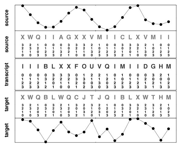
Figure 1: Transcription scheme for sequence length $L=4$. Symbols in light grey (source and target) correspond to the symbolic representations and the black symbols indicate the transcriptions that have to be applied to the upper symbols (source) to obtain the lower ones (target).

Ordinal patterns will be denoted by low case Greek letters throughout. Given two symbols $\alpha$ and $\beta$ there always exists a unique symbol $\tau_{\alpha,\beta}=\tau$, in the following called transcript, such that the composition $\tau\alpha=\beta$. Specifically if $\alpha=\left\langle j_{0},j_{1},\ldots,j_{L-1}\right\rangle$ and $\tau=\left\langle k_{0},k_{1},\ldots,k_{L-1}\right\rangle$, then the action of the symbol $\tau$ is defined as follows.

$$\tau\alpha=\left\langle j_{k_{0}},j_{k_{1}},\ldots,j_{k_{L-1}}\right\rangle.$$ (1)

Figure 1 shows symbolic representations of the ‘source’ and ‘target’ time series (light grey symbols) and the corresponding sequence of transcripts (black symbols) for $L=4$. With the operation (1), the set of ordinal $L$-patterns forms a finite non-Abelian group of order $L!$ known as the symmetric group $\mathcal{S}_{L}$ (i.e., the group of permutations on $L$ elements). The identity permutation is

$$id=\left\langle 0,1,...,L-1\right\rangle,$$

and the inverse element is given by

$$\alpha^{-1}=o(j_{0},...,j_{L-1}).$$

Then, $\tau_{\alpha,\beta}=\beta\alpha^{-1}$ and $\alpha=\tau_{\alpha,\beta}^{-1}\beta$ are equivalent definitions of the transcript $\tau_{\alpha,\beta}$. In sum, the use of transcripts allows us to exploit the structure of $\mathcal{S}_{L}$. For further properties of the transcripts, see Monetti2009 ; Amigo2012 .

We now focus on the probability function of transcripts. Consider a source and a target symbolic representations generated by the actual coupled dynamics of the time series. Given a data source, the set of all feasible ordinal $L$-patterns $\mathcal{S}^{1}=\{\alpha_{i}\}$ and $\mathcal{S}^{2}=\{\beta_{j}\}$ conform the state spaces of the source and the target representations, respectively. Let $\Pr(\alpha)$ and $\Pr(\beta)$ be the marginal probability functions, $\Pr(\alpha,\beta)$ the joint probability function, and

$$\Pr(\tau)=\sum_{\alpha,\beta\in\mathcal{S}_{L}:\;\beta\alpha^{-1}=\tau}\Pr(\alpha,\beta)$$ (2)

the probability function of the transcripts. Thus, the entropy of the joint probability function $\Pr(\alpha,\beta)$ and the entropy of the corresponding transcript probability function $\Pr(\tau)$ are given by

$$H(\alpha,\beta)=-\sum\limits_{\alpha,\beta\in\mathcal{S}_{L}}\Pr(\alpha,\beta)\log\Pr(\alpha,\beta),$$

and

$$H(\tau)=-\sum\limits_{\tau\in\mathcal{S}_{L}}\Pr(\tau)\log\Pr(\tau),$$

respectively.

The definition of transcript, Eq. (1), provides the algebraic relationship between source and target ordinal patterns. It follows that, given the triple $(\alpha,\beta,\tau)$, the knowledge of any pair of symbols, i.e. $(\alpha,\beta)$, $(\alpha,\tau)$, or $(\beta,\tau)$, univocally determines the remaining symbol. We call this the uniqueness property. This important property implies bookIT that the corresponding joint entropies coincide, i.e.,

$$H(\alpha,\beta)=H(\alpha,\tau)=H(\beta,\tau).$$ (3)

More generally, we mean by the uniqueness property the fact that different sets of variables comprised of ordinal patterns and transcripts contain the same information just because there is a 1-to-1 relation between any two of them, allowing to recover the variables of one set from the variables of the other. This property is used several times in the proofs of the Appendix.

3 Coupling complexity

Transcripts have triggered the development of information measures for the assessment of the coupling relationship between system components. The coupling complexity index is one of them. As its name indicates, this index aims at quantifying the complexity of the interaction. Here, we consider only one of two coupling complexity indices proposed in Amigo2012 , namely

$$C(\alpha,\beta)=\min\{H(\alpha),H(\beta)\}-\Delta(\alpha,\beta),$$ (4)

where

$$\Delta(\alpha,\beta)=H(\alpha,\beta)-H(\tau)$$ (5)

is the information loss of the transcription process Amigo2012 . According to (Amigo2012, , Corollary 1), $\Delta(\alpha,\beta)\geq 0$. Whenever we want to underscore the length of the ordinal patterns used in the symbolic representation, we will write $C_{L}$, $\Delta_{L}$, etc.

We clearly observe in (4) that the coupling complexity is symmetric under the interchange of $\alpha$ and $\beta$. By means of Eq. (3), $C$ can be written as

$$C(\alpha,\beta)=\min\{I(\alpha,\tau),I(\beta,\tau)\},$$ (6)

where $I$ denotes the mutual information. As mutual information is a non-negative quantity, it follows $C(\alpha,\beta)\geq 0$. Still a third expression is

$$C(\alpha,\beta)=H(\tau)-\max\{H(\alpha|\beta),H(\beta|\alpha)\}.$$ (7)

A generalization of (6)-(7) to the multivariate case can be found in the Appendix, Eqs. (A.11)-(A.12).

In order to deeper understand the meaning of $C$, we will discuss some cases leading to extreme values. Assume two identical but otherwise arbitrary time series. In this case, $\tau=id$ is the only existing transcript, thus $H(\tau)=0$. Since $H(\alpha,\beta)=H(\alpha)=H(\beta)$, we conclude that $C(\alpha,\beta)=0$. As a second example, consider a symbolic representation $\{\alpha_{t}\}_{t\geq 1}$ of a time series generated by random $iid$ numbers along with another arbitrary one, $\{\beta_{t}\}_{t\geq 1}$, independent of $\{\alpha_{t}\}_{t\geq 1}$. Since the time series are independent, $H(\alpha,\beta)=H(\alpha)+H(\beta)$. By assumption, the probability function $\Pr(\alpha)$ is uniform and, owing to the independence between $\alpha$ and $\beta$, the probability function $\Pr(\tau)$ is uniform as well. Thus, $H(\tau)=H(\alpha)$ and $\min\{H(\alpha),H(\beta)\}=H(\beta)$, hence $C(\alpha,\beta)=0$ once again. We have shown with these two examples that the coupling complexity is a property of the relationship between symbolic representations rather than a characteristic of the individual components. It certainly vanishes if the synchronization is rigid, but it also vanishes if the time series are independent, provided that at least one of them is equidistributed.

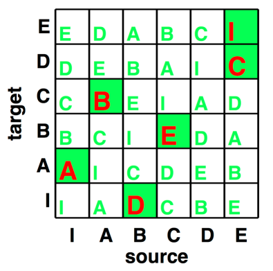
Figure 2: Transcription probability matrix for pattern length $L=3$ showing a rare case with high coupling complexity. Symbols and transcripts were denoted by the letters $I=\langle 0,1,2\rangle$, $A=\langle 0,2,1\rangle$, $B=\langle 2,0,1\rangle$, $C=\langle 1,0,2\rangle$, $D=\langle 1,2,0\rangle$, and $E=\langle 2,1,0\rangle$. The matrix elements are the transcripts which transform the ‘source symbol’ into the ‘target symbol’. In this example, only the transcripts in the shaded squares are supposed to have positive and equal probability. Correspondingly, only some pairs of symbols $(\alpha,\beta)$ are realized.

The example of Fig. 2 shows a transcription probability matrix for pattern length $L=3$, where every transcript $\tau$ in a shaded square connects only one pair of ordinal patterns $(\alpha,\beta)$, where $\alpha,\beta,\tau\in\{I,A,B,C,D,E\}$, while other connections are forbidden (more details in the caption of Fig. 2). Furthermore, the allowed pairs occur all with the same frequency. Thus, the knowledge of a transcript univocally determines one pair of symbols, i.e. there is no loss of information in the transcription process. Using this configuration, it is easy to calculate the coupling complexity index. We first observe that $H(\tau)=H(\alpha,\beta)=\log 3!$, hence $\Delta(\alpha,\beta)=0$. It is now clear why the term $\Delta$ in Eq. (4) was associated to the information loss of the transcription, which is zero in this particular case. Consequently, the coupling complexity reduces to $C(\alpha,\beta)=\min\{H(\alpha),H(\beta)\}=\log 3!-(2\log 2)/3!$, which is the maximum attainable complexity value for $L=3$ and $\Delta_{L}=0$. A proof for $C_{L}(\alpha,\beta)\leq$ $\log L!-(2\log 2)/L!$ if $\Delta_{L}=0$ can be found for $N$ symbolic representations in the Appendix, Proposition 2. This result strongly suggests that $\log L!$ is not an optimal upper bound for the coupling complexity index either in the bivariate nor in the multivariate case.

Figure 3 shows two examples again for the case $L=3$, which further clarify not only the meaning of $\Delta(\alpha,\beta)$ but also the difference between $C(\alpha,\beta)$ and $I(\alpha,\beta)$, the mutual information of the symbolic representations. Since every row and every column of the transcription probability matrices is occupied once and the probability is supposed to be the same, we obtain $I(\alpha,\beta)=\log 3!$ in both cases. In order to calculate $C(\alpha,\beta)$, we first note that both marginal entropies are equal, and the joint entropy also equals the marginal ones, i.e. $H(\alpha,\beta)=H(\alpha)=H(\beta)$. Consequently, the complexity index reduces to $C(\alpha,\beta)=H(\tau)$ in both examples. In the left panel of Fig. 3, we observe that only five transcripts are realized, four of them having a 1-to-1 relationship with pairs of source and target symbols, while the remaining one ($I$) is assigned to two different pairs. This situation is reflected by the information loss of the transcription, whose value is $\Delta(\alpha,\beta)=(2\log 2)/3!$; the complexity index amounts to $C(\alpha,\beta)=\log 3!-(2\log 2)/3!$. Observe that this value of $C$ is the same as we found for the transcription probability matrix of Fig. 2, but both cases are distinguished by the information loss $\Delta$. In the right panel of Fig. 3, the situation is different, with only four transcripts realized, three of them having a 1-to-1 relation with pairs of source and target symbols, the remaining one ($I$) being assigned to three different pairs. Now, the information loss of the transcription increases to $\Delta(\alpha,\beta)=(3\log 3)/3!$, while the complexity decreases to $C(\alpha,\beta)=\log 3!-(3\log 3)/3!$.

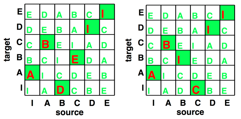
Figure 3: Transcription probability matrices for pattern length $L=3$ indicating two cases leading to different values of $C(\alpha,\beta)$ but the same mutual information $I(\alpha,\beta)$. Symbols are defined as in Fig. 2. As before, only the transcripts in the shaded squares are supposed to have positive and equal probability.

The coupling complexity index can be generalized to the multivariate case by means of the expression

$$C(\alpha^{1},\alpha^{2},\ldots,\alpha^{N})$$

$$= \min_{1\leq n\leq N}H(\alpha^{n})-[H(\alpha^{1},\alpha^{2},\ldots,\alpha^{N})-H(\tau^{1,2},\tau^{2,3},\ldots,\tau^{(N-1),N})],$$

where $\alpha^{n}$ denotes the feasible symbols of the $n^{\mbox{th}}$ time series and $\tau^{(n-1),n}$ are the transcripts connecting the symbols $\alpha^{n-1}$ and $\alpha^{n}$, i.e., $\tau^{(n-1),n}=\tau_{\alpha^{n-1},\alpha^{n}}$ for brevity. Similarly to the bivariate case, the generalized coupling complexity is invariant under the interchange of the $\alpha^{n}$’s. This property, which is a consequence of the uniqueness property explained before, is proved in Proposition 3 of the Appendix. For instance, consider three symbolic representations $\{\alpha_{t}\}_{t\geq 1}$, $\{\beta_{t}\}_{t\geq 1}$, and $\{\gamma_{t}\}_{t\geq 1}$, and all possible transcripts $\{(\tau_{\alpha,\beta})_{t}\}_{t\geq 1}$, $\{(\tau_{\alpha,\gamma})_{t}\}_{t\geq 1}$, and $\{(\tau_{\beta,\gamma})_{t}\}_{t\geq 1}$. The property of uniqueness warranties that $H(\tau_{\alpha,\beta},\tau_{\alpha,\gamma})=H(\tau_{\alpha,\beta},\tau_{\beta,\gamma})=H(\tau_{\alpha,\gamma},\tau_{\beta,\gamma})$ and therefore the invariance of $C(\alpha,\beta,\gamma)$ (see Eq. (3)) under permutations of its arguments.

Another consequence of the uniqueness property is the validity of Eq. (3) in higher dimensions, that is,

$$H(\alpha^{1},\alpha^{2},\ldots,\alpha^{N})=H(\alpha^{n},\tau^{1,2},\tau^{2,3},\ldots,\tau^{(N-1),N})$$ (9)

where $n\in\{1,\ldots,N\}$. Using property (9) and the following inequality (see for instance bookIT ),

$$H(Z|X,Y)\leq H(Z|X),$$

one can show under certain conditions the monotonicity of $C(\alpha^{1},\ldots,\alpha^{N})$ with respect to the number of variables, that is

$$C(\alpha^{1},...,\alpha^{k},\ldots,\alpha^{N})\geq C(\alpha^{1},...,\hat{\alpha}^{k},\ldots,\alpha^{N}),$$ (10)

where $\hat{\alpha}^{k}$ means that $\alpha^{k}$ has been omitted at that position, and $N\geq 3$. For further details, see Proposition 4 in the Appendix.

Figure 4: Coupling complexity indices evaluated for the coupled system defined in Eq. (11). The diagram shows the behaviour of the index of the three variables and the indices of all combinations of two variables versus the coupling $k_{yz}$ for $k_{xy}=1$. The full, dot-dashed, dashed, and dotted curves correspond to the complexities $C_{xyz}$, $C_{xy}$, $C_{yz}$, and $C_{xz}$, respectively. The symbolic representations were generated using ordinal patterns of length $L=4$ and time delay $T=6$ for time series with $N=5\mbox{x}10^{5}$ data points.

As an example, consider the following three delay-coupled autoregressive models,

$$x(t+1) = ax(t)+k_{xy}y(t-\Lambda_{xy})+\eta^{x}(t),$$ (11)

$$y(t+1) = by(t)+k_{yz}z(t-\Lambda_{yz})+\eta^{y}(t),$$

$$z(t+1) = cz(t)+\eta^{z}(t),\;\;\mbox{for}\;t\geq\max(\Lambda_{xy},\Lambda_{yz})$$

where $a=0.6$, $b=0.4$, $c=0.9$, $\Lambda_{xy}=3$, $\Lambda_{yz}=1$, and $\eta^{x},\eta^{y},\eta^{z}$ are normal random numbers satisfying $\left\langle\eta^{r}(t_{i})\eta^{s}(t_{j})\right\rangle=\delta_{rs}\delta_{ij}$ with $r,s\in\{x,y,z\}$. Here, we set the coupling constant $k_{xy}=1$ and $k_{yz}\in(-1,1)$. The components of this system are unidirectionally coupled in the form $z\rightarrow y\rightarrow x$, as clearly indicated by Eq. (11). Denote by $\alpha^{x},\alpha^{y},\alpha^{z}$ the symbols realized by the $x$-, $y$-, $z$-time series, respectively. Figure 4 shows that $C_{xyz:}:=C(\alpha^{x},\alpha^{y},\alpha^{z})\geq C(\alpha^{r},\alpha^{s})=:C_{rs}$, for every $r,s\in\{x,y,z\}$, $r\neq s$, in agreement with Eq. (10). It should be noted that for $k_{yz}=0$, the components $y$ and $z$ become uncoupled but the components $x$ and $y$ remain always coupled since $k_{xy}=1$. Furthermore, due to the coupling structure of the model, the components $x$ and $z$ become uncoupled for $k_{yz}=0$ as well. Figure 4 shows that for $k_{yz}=0$ both coupling complexities $C_{yz}$, and $C_{xz}$ almost vanish. However, $C_{xy}$ remains significantly positive due to the non-vanishing interaction between $x$ and $y$. It is worth noting that $C_{xyz}\simeq C_{xy}$ for $k_{yz}=0$, since the interaction $x$-$y$ is then the only source of coupling complexity in the system. Let us point out that the coincidence of $C_{xyz}$ with $C_{xy}$ in the uncoupled case ($k_{yz}=0$) is not valid in general (see Appendix, Proposition 5, with $N=3$, $\alpha^{1}=\alpha^{x}$, $\alpha^{2}=\alpha^{y}$, $\alpha^{3}=\alpha^{z}$). However, in many cases the use of a suitable time delay $T$ ($T$ is expressed in samples of the time series, see Fig. 4) may cause that the necessary conditions for the validity of this property are fulfilled, thus clearly unveiling the coupling structure of the dynamical system.

4 Applications to real world data

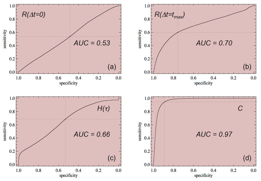
Figure 5: Receiver operator characteristic analysis to compare the performance of different linear and non-linear measures to distinguish pre-ictal from ictal states. The performance is quantified in terms of the area under the curve $AUC$, where $AUC=0.5$ is the expected performance of a random classifier. All plots show sensitivity versus specificity. a) Cross correlation $R$ evaluated at a time delay $\Delta t=0$. b) Maximum value of the cross correlation. c) The entropy $H(\tau)$ of the transcripts. d) The coupling complexity $C$. More details in the text.

We analyze the electrical brain activity of an infant patient suffering from frontal lobe epilepsy (FLE). It should be remarked that it is not the purpose of this work to perform a clinical study but to demonstrate the applicability of the above presented methodology to an example of real world data. A clinical study of the evolution of the brain electrical activity of this infant during therapy has already been presented in Bunk et al. Bunk . The authors compared the performance of a variety of synchronization measures and found that the synchronization level is significantly increased during the clinical manifestation of FLE, even in interictal periods. The EEG recording was acquired during a time interval of 15 minutes at a sampling rate of 250 Hz and a signal depth of 16 bits, and consists of 21 synchronously obtained time series. The positioning of the electrodes followed that of the standardized 10-20-International System of Electrode Placements (see the left panel of Fig. 6). In Amigo2012 , we demonstrated the applicability of the coupling complexity index $C$ to EEG data in the context of epilepsy studies. By means of a sliding window analysis considering all possible electrode pairs, we showed that $C$ increases in ictal periods, meaning that the relationship between different EEGs becomes less random.

Here, we consider a simple task, namely, that of differentiating pre-ictal and ictal states, in order to evaluate the performance of $C$ in comparison with other linear and non-linear correlation measures. To this end, we perform a sliding window analysis including all possible pairs of EEG signals (210 pairs), using windows of size $w\simeq 16\sec$ and sampling every $\Delta w\simeq 2\sec$. We have used patterns of length $L=4$ and a time delay $T=0.048\sec$, thus every symbol has a time horizon of $\Delta T=0.144\sec$. For every measure, all values in the pre-ictal and ictal states are collected for all pairs, respectively. Then, the performance is evaluated by means of a receiver operator characteristic analysis Swets1986 . Figure 5 shows plots of the sensitivity versus the specificity for the cross-correlations $R(\Delta t=0)$ and $R(\Delta t=t_{\max})$, the entropy of the transcripts $H(\tau)$, and the coupling complexity $C$. Here, $\Delta t$ denotes the time lag and $t_{\max}$ is the time lag at the maximum of $R$. The sensitivity is defined as $sen=\frac{Ntp}{Ntp+Nfn}$, where $Ntp$ is the number of true positives and $Nfn$ is the number of false negatives. Similarly, the specificity is given by the fraction $sp=\frac{Ntn}{Ntn+Nfp}$, where $Ntn$ is the number of true negatives and $Nfp$ is the number of false positives. Thus, for a random classifier, sensitivity and specificity amount about the same, and the area under the curve (AUC) becomes $AUC\simeq 0.5$. Figure 5 (a) indicates that the cross-correlation $R(\Delta t=0)$ has a rather poor performance, quite close to that of the random classifier. The performance of the cross-correlation improves when considering the maximum $R(\Delta t=t_{\max})$, where now the brain state can be correctly predicted in 70$\%$ of the cases. The entropy $H(\tau)$ has a performance rather smaller than that of $R(\Delta t=t_{\max})$, but the best performance is given by $C$ with an $AUC=0.97$. Thus, this example shows that $C$ captures the main features essential to distinguish between these two brain states.

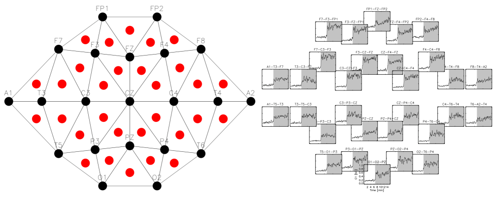
Figure 6: Left: Two dimensional diagram representing a two dimensional projection of the position of the electrodes (black points, vertices of the triangles) on the head, oriented as up-down $\rightarrow$ frontal-occipital, left-right $\rightarrow$ left ear - right ear. Right: The time evolution of the complexity $C$ evaluated for every electrode triple. The positions of the responses correspond to the grey points centered on the triangles. All insets are displayed using the same scale, thus they can easily be compared. The symbolic representations were generated using ordinal patterns of length $L=3$ and time delay $T=0.048\sec$. More details in text.

The application of $C$ to the multivariate case (Eq. (3)) has to be done with some care due to the curse of dimensionality. In fact, given $N$ time series the number of possible states for the joint process (transcripts) is $L!^{N}$ ($L!^{N-1}$), respectively. Thus, one has to find a suitable compromise between the number $N$ of time series to be analyzed and the length $L$ of the ordinal patterns. We consider a trivariate analysis of the above EEG data, where we have chosen neighboring triples of electrodes as shown in the left panel of Fig 6. Using $L=3$, a rough estimate of the necessary data to perform such an analysis leads to $10\,\mbox{x}\,3!^{3}\simeq 2160$ data points, which is well below the window length of $w=16\sec=4000$ data points used in this study. The right panel of Fig. 6 shows for every electrode triple the time evolution of the complexity $C$, where in every inset the white (grey) region corresponds to the pre-ictal (ictal) state, respectively. Note that the positions of the insets correspond to that of the central, grey points of the triangles on the left panel of the same figure. We first observe in all insets that $C$ increases in the ictal state, in agreement with the results of the bivariate analysis Amigo2012 . Furthermore, Fig. 6 shows that $C$ displays the strongest contrasts in the frontal region, thus supporting the clinical diagnosis of frontal lobe epilepsy.

5 Coupling complexity rate

Consider $N$ stationary random processes $\mathbf{X}^{n}=\{X_{t}^{n}\}_{t\geq 1}$, $1\leq n\leq N$, where the identically distributed random variables $X_{t}^{n}$ take values in a linearly ordered set. For each $t\geq 1$ and $L\geq 2$, set $\alpha_{t}^{n}=o(X_{t}^{n},...,X_{t+L-1}^{n})\in\mathcal{S}_{L}$. Therefore, each sequence $\mathbf{A}^{n}=\{\alpha_{t}^{n}\}_{t\geq 1}$ is a stationary and identically distributed random process taking values in $\mathcal{S}_{L}$.

For each $n$, let $H(X^{n})$ be the entropy of the (identically distributed) random variables $X_{t}^{n}$ and

$$h(\mathbf{X}^{n})=\lim_{t\rightarrow\infty}\frac{1}{t}H(X_{1}^{n},...,X_{t}^{n})$$

the entropy rate of the process $\mathbf{X}^{n}$. The entropy $H_{L}(\alpha^{n}):=H(o(X_{1}^{n},...,X_{L}^{n}))$, is called the permutation entropy of order $L$ corresponding to the common probability distribution of the $\alpha_{t}^{n}$’s, and

$$h(\mathbf{A}^{n})=\lim_{L\rightarrow\infty}\frac{1}{L}H_{L}(\alpha^{n})=:h^{\ast}(\mathbf{X}^{n})$$ (12)

is the permutation entropy rate of the process $\mathbf{X}^{n}$. It can be proved that if the alphabet of $\mathbf{X}^{n}$ is finite, then $h^{\ast}(\mathbf{X}^{n})=h(\mathbf{X}^{n})$ Amigo2012a ; Haruna2011 .

In (A.6)-(A.7) we have defined the coupling complexity index $C_{L}(\alpha^{1},...,\alpha^{N})$ for random ordinal $L$-patterns $\alpha^{1},...,\alpha^{N}$. According to (12), $H_{L}(\alpha^{n})$ scales linearly with $L$, and the same happens with $C_{L}(\alpha^{1},...,\alpha^{N})$ for $N$ fixed (see (3)). Therefore, we define the corresponding coupling complexity rate for symbolic processes as

$$C_{L}(\mathbf{A}^{1},...,\mathbf{A}^{N})=\underset{L\rightarrow\infty}{\lim\sup}\frac{1}{L}C_{L}(\alpha^{1},...,\alpha^{N}).$$ (13)

This scenario can be extended to time series output by chaotic dynamical systems (with sufficiently regular invariant measures). One important difference between the randomly generated time series and the deterministically generated ones is the existence in the latter case of so-called forbidden patterns (i.e., ordinal patterns that cannot occur) under very general conditions Amigo2006 ; Amigo2008 ; Amigo2010 . The bottom line is that the number of ordinal $L$-patterns actually observed does not grow factorially but exponentially with $L$. To be specific, $\left|\{\alpha\in\mathcal{S}_{L}:\Pr(\alpha)>0\}\right|\propto e^{Lh_{top}(f)}$, where $\propto$ stands for “asymptotically”, and $h_{top}(f)$ denotes the topological entropy of $f$. Hence, if $h_{top}(f)<\infty$,

$$C_{L}(\alpha^{1},...,\alpha^{N})\leq\min_{1\leq n\leq N}H_{L}(\alpha^{n})\leq Lh_{top}(f),$$ (14)

We conclude that if $\{\alpha_{t}^{n}\}_{t\geq 1}$ proceeds from an orbit generated by a map $f:I^{d}\rightarrow I^{d}$, then

$$\frac{1}{L}C_{L}(\alpha^{1},...,\alpha^{N})\leq\frac{1}{L}\cdot Lh_{top}(f)=h_{top}(f).$$

Then $C(\mathbf{A}^{1},...,\mathbf{A}^{N})<\infty$ if $h_{top}(f)<\infty$.

6 Conclusion

In this paper we have briefly reviewed the concept of transcript and some of its properties. We have also presented a detailed discussion of the coupling complexity index, using examples that clarify its meaning. Furthermore, we introduced a generalization of this index to $N$ time series and discussed several useful properties via examples. A formal approach to the $N$-variate coupling complexity index, containing mathematical proofs of some of its properties, can be found in the Appendix below. As an application in higher dimensions, we evaluated the coupling complexity index in a trivariate case using biomedical data and found agreement with the results obtained in the bivariate analysis. In the last section we introduced the coupling complexity rate of symbolic random processes.

Appendix A Properties of the $N$-variate coupling complexity index

Two trivial properties of the transcripts are

$$\tau_{\beta,\alpha}=(\tau_{\alpha,\beta})^{-1}$$ (A.1)

and

$$\tau_{\beta,\gamma}\tau_{\alpha,\beta}=\gamma\beta^{-1}\beta\alpha^{-1}=\gamma\alpha^{-1}=\tau_{\alpha,\gamma}.$$ (A.2)

Given the random variables $\alpha^{n}$, $1\leq n\leq N$, with outcomes in $\mathcal{S}_{L}$, then

$$H(...,\alpha^{n},\alpha^{n+1},...) =H(...,\alpha^{n},\tau_{\alpha^{n},\alpha^{n+1}},...)=H(...,\alpha^{n},\tau_{\alpha^{n+1},\alpha^{n}},...)$$ (A.3)

$$=H(...,\tau_{\alpha^{n},\alpha^{n+1}},\alpha^{n+1},...)=H(...,\tau_{\alpha^{n+1},\alpha^{n}},\alpha^{n+1},...)$$ (A.4)

because any of the random variable pairs explicitly shown in (A.3)-(A.4) can be determined from any other variable pairs.

For notational convenience we will also use the notations $\tau^{n,n+1}$ or $\tau(\alpha^{n},\alpha^{n+1})$ for $\tau_{\alpha^{n},\alpha^{n+1}}$, and write, for example,

$$H(\tau_{\alpha^{1},\alpha^{2}},...,\tau_{\alpha^{N-1},\alpha^{N}})\equiv H(\tau^{1,2},...,\tau^{N-1,N})\equiv H(\tau(\alpha^{1},\alpha^{2}),...,\tau(\alpha^{N-1},\alpha^{N})).$$

If all ordinal $L$-patterns $\alpha^{1},...,\alpha^{N}$ are feasible, then the $L!^{N-1}$ sets

$$\Omega_{L}(\tau^{1,2},...,\tau^{N-1,N})$$

$$= \{(\alpha^{1},...,\alpha^{N})\in(\mathcal{S}_{L})^{N\text{ }}:\tau^{1,2}\alpha^{1}=\alpha^{2},...,\tau^{N-1,N}\alpha^{N-1}=\alpha^{N}\},$$

build a partition of $(\mathcal{S}_{L})^{N\text{ }}$, with $\left|\Omega_{L}(\tau^{1,2},...,\tau^{N-1,N})\right|=L!$, independently of $N$. Actual time series may have symbolic representations with forbidden patterns Amigo2006 ; Amigo2008 ; Amigo2010 . This may entail that $\left|\Omega_{L}(\tau^{1,2},...,\tau^{N-1,N})\right|<L!$, or even $\Omega_{L}(\tau^{1,2},...,\tau^{N-1,N})=\emptyset$ for some choices of $\tau^{1,2},...,\tau^{N-1,N}$.

Consider throughout $N\geq 2$ random variables $\alpha^{n}$, $1\leq n\leq N$, taking values in $\mathcal{S}_{L}$, sometimes called random ordinal $L$-patterns. Their coupling complexity index was defined Amigo2012 as

$$C_{L}(\alpha^{1},...,\alpha^{N})=\min_{1\leq n\leq N}H_{L}(\alpha^{n})-\Delta_{L}\left(\alpha^{1},...,\alpha^{N}\right),$$ (A.6)

where $H_{L}(\cdot)$ stands for the Shannon entropy of the random ordinal $L$-patterns appearing in the argument, and

$$\Delta_{L}\left(\alpha^{1},...,\alpha^{N}\right)=H_{L}(\alpha^{1},...,\alpha^{N})-H_{L}(\tau^{1,2},...,\tau^{N-1,N})$$ (A.7)

is called the transcription information loss Amigo2012 . According to (Amigo2012, , Corollary 1), $\Delta(\alpha,\beta)\geq 0$. We dispense with the lower indices $L$ for the time being.

We are going to give an alternative expression for $C(\alpha^{1},...,\alpha^{N})$ that, in passing, will also prove that it is non-negative. First of all, from

$$H(\alpha^{1},...,\alpha^{N})=H(\alpha^{k},\tau^{1,2},...,\tau^{N-1,N})$$ (A.8)

it follows

$$\Delta\left(\alpha^{1},...,\alpha^{N}\right)=H(\alpha^{k}\left|\tau^{1,2},...,\tau^{N-1,N}\right),$$ (A.9)

$1\leq k\leq N$. Since $\Delta\left(\alpha^{1},...,\alpha^{N}\right)$ does not depend on $k$, the following result holds.

Proposition 1

$H\left(\alpha^{i}\right|\tau^{1,2},...,\tau^{N-1,N})=H\left(\alpha^{j}\right|\tau^{1,2},...,\tau^{N-1,N})$, for every $1\leq i,j\leq N$.

Therefore,

$$C(\alpha^{1},...,\alpha^{N}) =\min_{1\leq n\leq N}H(\alpha^{n})-H(\alpha^{k}\left|\tau^{1,2},...,\tau^{N-1,N}\right)$$ (A.10)

$$=\min_{1\leq n\leq N}\left\{H(\alpha^{n})-H(\alpha^{k}\left|\tau^{1,2},...,\tau^{N-1,N}\right)\right\}$$

$$=\min_{1\leq n\leq N}\left\{H(\alpha^{n})-H(\alpha^{n}\left|\tau^{1,2},...,\tau^{N-1,N}\right)\right\}$$

$$=\min_{1\leq n\leq N}I(\alpha^{n};\tau^{1,2},...,\tau^{N-1,N})\geq 0.$$ (A.11)

Still other expression is

$$C(\alpha^{1},...,\alpha^{N}) =H(\tau^{1,2},...,\tau^{N-1,N})-\left(H(\alpha^{1},...,\alpha^{N})-\min_{1\leq n\leq N}H(\alpha^{n})\right)$$

$$=H(\tau^{1,2},...,\tau^{N-1,N})-\max_{1\leq n\leq N}H\left(\alpha^{1},...,\hat{\alpha}^{n},...,\alpha^{N}\right|\left.\alpha^{n}\right),$$ (A.12)

where $\hat{\alpha}^{n}$ means that $\alpha^{n}$ has been omitted at that position.

A trivial upper bound of $C(\alpha^{1},...,\alpha^{N})$ is $\log L!.$ The next result suggests that this bound is not optimal.

Proposition 2

If $\Delta\left(\alpha^{1},...,\alpha^{N}\right)=0$, then

$$C(\alpha^{1},...,\alpha^{N})=\min_{1\leq n\leq N}H(\alpha^{n})\leq\log L!-\frac{2}{L!}\log 2.$$

Proof. Suppose first $N\ =2$. In order that $\Delta(\alpha^{1},\alpha^{2})=0$ there must be a 1-to-1 relation between each realization $(\alpha_{i},\alpha_{j})$ of the pair $(\alpha^{1},\alpha^{2})$ and the ensuing transcript $\tau_{i,j}=\alpha_{j}(\alpha_{i})^{-1}$, i.e., $\left|\Omega_{L}(\tau)\right|=1$ for every $\tau\in\mathcal{S}_{L}$.

In turn, if given, say, any realization $\alpha_{i}$ of $\alpha^{1}$ there would exist one and only one realization $\tau_{i,j}$ of $\tau^{1,2}$, then this would fix also the realization $\alpha_{j}$ of $\alpha^{2}$ so that $H(\alpha^{1},\alpha^{2})=H(\alpha^{1})=H(\alpha^{2})$, and $C(\alpha^{1},\alpha^{2})$ could reach its maximum $\log L!$. We prove by contradiction that this cannot happen.

A 1-to-1 relation $\alpha_{i}\leftrightarrow\tau_{i,j}$ (or $\alpha_{j}\leftrightarrow\tau_{i,j}=\tau_{j,i}^{-1}$ for that matter) means that if $\alpha_{1},...,\alpha_{L!}$ is an enumeration of the ordinal patterns in $\mathcal{S}_{L}$ (without restriction, $\alpha_{1}=\left\langle 1,2,...,L-1,L\right\rangle=:id$), then there is a permutation $\pi:\{1,...,L!\}\rightarrow\{1,...,L!\}$ such that

$$\alpha_{\pi(1)}(\alpha_{1})^{-1}=\tau_{1,\pi(1)},\;...,\;\alpha_{\pi(i_{0})}(\alpha_{i_{0}})^{-1}=id,\;...,\;\alpha_{\pi(L!)}(\alpha_{L!})^{-1}=\tau_{L!,\pi(L!)}$$ (A.13)

is also an enumeration of $\mathcal{S}_{L}$. Note that $\pi(i_{0})=i_{0}$ but $\pi(i)\neq i$ for $i\neq i_{0}$ because, otherwise, the identity $id$ would be repeated on the list (A.13).

We claim that such an enumeration is not possible. Indeed, from

$$\tau_{i,\pi(i)}\tau_{\pi(i),i}=\alpha_{\pi(i)}(\alpha_{i})^{-1}\alpha_{i}(\alpha_{\pi(i)})^{-1}=id$$

for every $i$, it follows that each of the $L!-1$ transcripts $\tau_{i,\pi(i)}$ with $i\neq i_{0}$ can be paired with its inverse $(\tau_{i,\pi(i)})^{-1}=\tau_{\pi(i),i}\neq\tau_{i,\pi(i)}$. Since their number is odd, this is not possible. It follows that there is at least one $i\in\{1,...,L!\}$ such that $\alpha_{i}$ is not realized by $\alpha^{1}$, hence $C(\alpha^{1},\alpha^{2})\leq H(\alpha^{1})<\log L!$.

We conclude from the above argument that the maximum of $C\left(\alpha^{1},\alpha^{2}\right)$ is reached when the would-be pairing $\alpha_{i}\leftrightarrow\tau_{i,j}$ is minimally violated, i.e., there is only one $\alpha_{i^{\prime}}$ with no correspondence $\tau_{i^{\prime},j}$ (thus the pattern $\alpha_{i^{\prime}}$ is not realized by $\alpha^{1})$, and there is only one $\alpha_{i^{\prime\prime}}$ with two correspondences $\tau_{i^{\prime\prime},k}$ and $\tau_{i^{\prime\prime},h}$. Without restriction, we assume that this happens for $i^{\prime}=L!$, and $i^{\prime\prime}=L!-1$, i.e., there is a map $\phi:\{1,...,L!-1\}\rightarrow\{1,...,L!\}$ with $\phi(i_{0})=i_{0}$, $\phi(i)\neq i$ for $i\neq i_{0}$, such that

$$\tau_{1,\phi(1)},\;...,\;\tau_{i_{0},\phi(i_{0})}=id,\;...,\;\tau_{L!-1,\phi(L!-1)},\;\tau_{L!-1,K},$$

is also an enumeration of $\mathcal{S}_{L}$, where $K\in\{1,...,L!\}$ is such that $K\neq\phi(i)$ for $i=1,...,L!-1$. To allow $H(\alpha^{1})$ to be as great as possible, suppose furthermore that the transcripts are uniformly distributed. Then

$$H(\alpha^{1})=-(L!-2)\frac{1}{L!}\log\frac{1}{L!}-\frac{2}{L!}\log\frac{2}{L!}=\log L!-\frac{2}{L!}\log 2,$$

$H(\alpha^{2})=\log L!$, and

$$C(\alpha^{1},\alpha^{2})=\min\{H(\alpha^{1}),H(\alpha^{2})\}=\log L!-\frac{2}{L!}\log 2.$$

Finally, in the case $N>2$ extend consecutively the above rigid correlations between $\alpha^{1}$ with $\alpha^{2}$ (which maximize $C(\alpha^{1},\alpha^{2})$) to $\alpha^{3},...,\alpha^{N}$. Then $\Delta(\alpha^{1},...,\alpha^{N})=0$, $H(\alpha^{1})=...=H(\alpha^{\left\lfloor N+1\right\rfloor})=\log L!-\frac{2}{L!}\log 2$, $H(\alpha^{2})=...=H(\alpha^{\left\lfloor N/2\right\rfloor})=\log L!$, and $C(\alpha^{1},...,\alpha^{N})=\min_{1\leq n\leq N}H(\alpha^{(n)})=\log L!-\frac{2}{L!}\log 2.$ $\square$

Next we derive some basic properties of the complexity index.

Proposition 3

(Invariance). $C(\alpha^{1},...,\alpha^{N})$ is invariant under permutations of $\alpha^{1},$ …, $\alpha^{N}$.

Proof. We claim that each random variable in the set $\mathcal{T}=\{\tau^{1,2},...,\tau^{N-1,N}\}$ is a function of random variables in the set $\mathcal{T}_{\pi}=\{\tau^{\pi(1),\pi(2)},...,\tau^{\pi(N-1),\pi(N)}\}$, and vice-versa, for any $\pi\in\mathcal{S}_{N}$. It follows then

$$H(\tau^{1,2},...,\tau^{N-1,N})=H(\tau^{\pi(1),\pi(2)},...,\tau^{\pi(N-1),\pi(N)}),$$

and also $C(\alpha^{1},...,\alpha^{N})=C(\alpha^{\pi(1)},...,\alpha^{\pi(N)})$ by the definition (A.6)-(A.7).

In fact, we are going to prove the somewhat stronger result that $\mathcal{T}_{\pi}$ generates all $\tau^{i,j}$, $1\leq i\neq j\leq N$, via multiplication of transcripts sharing a common index. To this end, multiply each transcript of $\mathcal{T}_{\pi}$ times the preceding one, that is, $\tau^{\pi(n),\pi(n+1)}\tau^{\pi(n-1),\pi(n)}=\tau^{\pi(n-1),\pi(n+1)}$ (see (A.2)), to obtain the set

$$\mathcal{T}_{\pi}^{(2)}=\left\{\tau^{\pi(n),\pi(n+2)}:\;1\leq n\leq N-2\right\}.$$

$\mathcal{T}_{\pi}^{(2)}$ is the first member of a family of sets

$$\mathcal{T}_{\pi}^{(k)}=\left\{\tau^{\pi(n),\pi(n+k)}:\;1\leq n\leq N-k\right\},$$

$2\leq k\leq N-1$, recursively constructed as follows. Define $\mathcal{T}_{\pi}^{(1)}=\mathcal{T}_{\pi}$ and multiply all transcripts $\tau^{\pi(n),\pi(n+i)}\in\mathcal{T}_{\pi}^{(i)}$, $1\leq i\leq k-1$, times all transcripts $\tau^{\pi(n-k+i),\pi(n)}\in\mathcal{T}_{\pi}^{(k-i)}$, sharing a common index $\pi(n)$ as indicated. According to (A.2),

$$\tau^{\pi(n),\pi(n+i)}\tau^{\pi(n-k+i),\pi(n)}=\tau^{\pi(n-k+i),\pi(n+i)}\in\mathcal{T}_{\pi}^{(k)}.$$

In particular, $\mathcal{T}_{\pi}^{(N-1)}=\left\{\tau^{\pi(1),\pi(N)}\right\}$.

By construction, $\mathcal{T}_{\pi}^{(1)},\mathcal{T}_{\pi}^{(2)},...,\mathcal{T}_{\pi}^{(N-1)}$ build a partition of the set $\{\tau^{\pi(n),\pi(m)}:1\leq n<m\leq N\}$ such that $\tau^{\pi(n),\pi(m)}\in\mathcal{T}_{\pi}^{(m-n)}$. The remaining transcripts are obtained by inversion (see (A.1)).

Consider now an arbitrary transcript $\tau^{i,j}$, and let $\pi(a)=i$ and $\pi(b)=j$. Suppose that $a<b$, otherwise consider $\tau^{j,i}=(\tau^{i,j})^{-1}$ instead. Then $\tau^{i,j}=\tau^{\pi(a),\pi(b)}\in\mathcal{T}_{\pi}^{(b-a)}$. We conclude that any transcript $\tau^{i,j}$ (in particular, those $\tau^{i,i+1}\in\mathcal{T}$) can be determined from $\mathcal{T}_{\pi}$ using algebraic operations (multiplications and inversions) in the way explained above.

For the inverse relation, set $\beta^{n}:=\alpha^{\pi(n)}$ and proceed as before, using this time the permutation $\pi^{-1}$, to show that the transcript $\tau(\beta^{n},\beta^{n+1})=\tau(\alpha^{\pi(n)},\alpha^{\pi(n+1)})$ can be recovered via algebraic operations from transcripts of $\{\tau(\beta^{(\pi^{-1}(1))},\beta^{(\pi^{-1}(2))}),$…, $\tau(\beta^{\pi^{-1}(N-1)},\beta^{\pi^{-1}(N)})\}=\{\tau(\alpha^{1},\alpha^{2}),...,\tau(\alpha^{N-1},\alpha^{N})\}$. $\square$

The next proposition shows that, under some provisos, $C$ is monotonous with respect to the number of random variables.

Proposition 4

(Monotonicity). Let $N\geq 3$.

(i)

If there is only one random variable $\alpha^{n_{\min}}$ such that $\min_{1\leq n\leq N}H(\alpha^{n})=H(\alpha^{n_{\min}})$, then $C(\alpha^{1},...,\alpha^{N})\geq C(\alpha^{1},...,\hat{\alpha}^{k},...,\alpha^{N})$ for all $k\neq n_{\min}$.

(ii)

If there are at least two random variables with minimum entropy, then $C(\alpha^{1},...,\alpha^{N})$ $\geq C(\alpha^{1}$,…,$\hat{\alpha}^{k}$,…,$\alpha^{N})$ for all $k=1,...,N$.

Proof. (i) If $k\neq n_{\min}$, then $\min_{n\neq k}H(\alpha^{n})=\min_{1\leq n\leq N}H(\alpha^{n})=H(\alpha^{n_{\min}})$. Then, using (A.9) and Proposition 1,

$$C(\alpha^{1},...,\alpha^{N})-C(\alpha^{1},...,\hat{\alpha}^{k},...,\alpha^{N})$$

$$=H\left(\alpha^{n_{\min}}\right|\tau^{1,2},...,\tau^{k-1,k+1},...\tau^{N-1,N})-H\left(\alpha^{n_{\min}}\right|\tau^{1,2},...,\tau^{N-1,N})$$

$$\geq 0$$

because the relative entropy $H(\alpha^{n_{\min}}\left|...\right)$ is greater the less conditioning variables.

(ii) In this case, one can always find for any $k\in\{1,...,N\}$ a random ordinal $L$-pattern $\alpha^{n}$ with $H(\alpha^{n})=H(\alpha^{n_{\min}})$ and $n\neq k$. Apply then (i). $\square$

Proposition 5

If $\alpha^{k}$ is independent of $\{\alpha^{1},...,\hat{\alpha}^{k},...,\alpha^{N}\}$ and $H(\alpha^{k})=\log L!$, then

$$C(\alpha^{1},...,\alpha^{N})=C(\alpha^{1},...,\hat{\alpha}^{k},...,\alpha^{N}),$$

where, in case $N=2$, we set $C(\alpha^{1})=C(\alpha^{2})=0$.

Proof. The case $N=2$ has to be dealt with separately. If, say, $k=1$, then $\min\{H(\alpha^{1}),$ $H(\alpha^{2})\}=H(\alpha^{2})$, $H(\alpha^{1},\alpha^{2})=H(\alpha^{1})+H(\alpha^{2})$ by assumption, and

$$\Pr(\tau) = \sum_{\alpha^{1},\alpha^{2}:\tau\alpha^{1}=\alpha^{2}}\Pr(\alpha^{1},\alpha^{2})=\sum_{\alpha^{1}}\Pr(\alpha^{1})\Pr(\tau\alpha^{1})$$

$$= \frac{1}{L!}\sum_{\alpha^{1}}\Pr(\tau\alpha^{1})=\frac{1}{L!},$$

hence $H(\tau)=\log L!=H(\alpha^{1})$. It follows $C(\alpha^{1},\alpha^{2})=0=:C(\alpha^{2}).$

Suppose $N\geq 3$. Since $C(\alpha^{1},...,\alpha^{N})\geq C(\alpha^{1},...,\hat{\alpha}^{k},...,\alpha^{N})$ by Proposition 4 (ii), we need only to show that $C(\alpha^{1},...,\alpha^{N})\leq C(\alpha^{1},...,\hat{\alpha}^{k},...,\alpha^{N})$.

Using $\min_{1\leq n\leq N}H(\alpha^{n})=\min_{n\neq k}H(\alpha^{n})$ and

$$H(\alpha^{1},...,\alpha^{N})=H(\alpha^{k})+H(\alpha^{1},...,\hat{\alpha}^{k},...,\alpha^{N}),$$

we obtain

$$C(\alpha^{1},...,\alpha^{N})-C(\alpha^{1},...,\hat{\alpha}^{k},...,\alpha^{N})$$

$$=-H(\alpha^{1},...,\alpha^{N})+H(\alpha^{1,2},...,\tau^{N-1,N})$$

$$+H(\alpha^{1},...,\hat{\alpha}^{k},...,\alpha^{N})-H(\tau^{1,2},...,\tau^{k-1,k+1},\tau^{N-1,N})$$

$$=-H(\alpha^{k})+H(\tau^{1,2},...,\tau^{N-1,N})-H(\tau^{1,2},...,\tau^{k-1,k+1},\tau^{N-1,N}),$$

where

$$H(\tau^{1,2},...,\tau^{N-1,N})=H(\tau^{n,k},\tau^{1,2},...,\tau^{k-1,k+1},\tau^{N-1,N})$$

for any $n\neq k$. Then

$$C(\alpha^{1},...,\alpha^{N})-C(\alpha^{1},...,\hat{\alpha}^{k},...,\alpha^{N})$$

$$=-H(\alpha^{k})+H(\tau^{n,k}\left|\tau^{1,2},...,\tau^{k-1,k+1},\tau^{N-1,N}\right)\leq 0$$

because $H(\tau^{n,k}\left|\tau^{1,2},...,\tau^{k-1,k+1},\tau^{N-1,N}\right)\leq\log L!=H(\alpha^{k})$. $\square$

If all the random variables $\alpha^{n}$ have a flat probability distribution ($H(\alpha^{1})=...=H(\alpha^{1})=\log L!$), then, according to Proposition 2, $\Delta(\alpha^{1},...,\alpha^{N})>0$ and

$$C(\alpha^{1},...,\alpha^{N})=\log L!-\Delta(\alpha^{1},...,\alpha^{N})<\log L!\text{.}$$ (A.14)

The next proposition is a strengthening of (A.14).

Proposition 6

If all the random ordinal $L$-patterns $\alpha^{n}$ are independent and uniformly distributed ($H(\alpha^{1})=...=H(\alpha^{1})=\log L!)$, then $C(\alpha^{1},...,\alpha^{N})=0$.

Proof. We have to prove (see (A.14)), that $\Delta(\alpha^{1},...,\alpha^{N})=\log L!$.

First of all,

$$H(\alpha^{1},...,\alpha^{N})=H(\alpha^{1})+...+H(\alpha^{N})=N\log L!$$ (A.15)

because $\alpha^{1},...,\alpha^{N}$ are independent. Then (remember (A)),

$$\Pr(\tau^{1,2},...,\tau^{N-1,N}) =\sum_{(\alpha^{1},...,\alpha^{N})\in\Omega_{L}(\tau^{1,2},...,\tau^{N-1,N})}\Pr(\alpha^{1},...,\alpha^{N})$$

$$=\sum_{(\alpha^{1},...,\alpha^{N})\in\Omega_{L}(\tau^{1,2},...,\tau^{N-1,N})}\Pr(\alpha^{1})\cdots\Pr(\alpha^{N})$$

$$=\sum_{(\alpha^{1},...,\alpha^{N})\in\Omega_{L}(\tau^{1,2},...,\tau^{N-1,N})}\frac{1}{(L!)^{N}}=\frac{1}{(L!)^{N-1}},$$

where we have used $\left|\Omega_{L}(\tau^{1,2},...,\tau^{N-1,N})\right|=L!$ in the last equality. We conclude that the multivariate random variable $\tau^{1,2},...,\tau^{N-1,N}$ is also uniformly distributed. Hence

$$H(\tau^{1,2},...,\tau^{N-1,N})=\log(L!)^{N-1}=(N-1)\log L!.$$ (A.16)

Finally, from (A.15) and (A.16),

$$\Delta(\alpha^{1},...,\alpha^{N})=H(\alpha^{1},...,\alpha^{N})-H(\tau^{1,2},...,\tau^{N-1,N})=\log L!\text{ }\square$$

Received xxxx 20xx; revised xxxx 20xx.

References

• (1) L. Glass, Nature 410, (2001) 277
• (2) G. Tononi and G.E. Edelman, Science 282, (1998) 1846
• (3) S.H. Strogatz, et al., Nature 438, (2005) 43
• (4) C. Bandt and B. Pompe, Phys. Rev. Lett. 88, (2002) 174102
• (5) J.M. Amigó and M.B. Kennel, Physica D 231, (2007) 137
• (6) M. Staniek and K. Lehnertz, Phys. Rev. Lett., 100, (2008) 158101
• (7) R. Monetti, W. Bunk, T. Aschenbrenner, and F. Jamitzky, Phys. Rev. E 79, (2009) 046207
• (8) J.M. Amigó, R. Monetti, T. Aschenbrenner, and W. Bunk, Chaos 22, (2012) 013105
• (9) T.M. Cover and J.A. Thomas, Elements of Information Theory, John Wiley & Sons, New York (1991)
• (10) W. Bunk, T. Aschenbrenner, et al., (2009) e-print arXiv:physics.med-ph/0905.3911v1
• (11) J.A. Swets, Psycological Bulletin 99, (1986) 100
• (12) J.M. Amigó, Physica D 241, (2012) 789
• (13) T. Haruna and K. Nakajima, Physica D 240, (2011) 1370
• (14) J.M. Amigó, L. Kocarev, J. Szczepanski, Phys. Lett. A 355, (2006) 27
• (15) J.M. Amigó and M.B. Kennel, Physica D 237, (2008) 2893
• (16) J.M. Amigó, Permutation Complexity in Dynamical Systems: Ordinal Patterns, Permutation Entropy, and All That (Springer Verlag, Berlin, 2010)