Mapping the Central Region of the PPN CRL 618 at Sub-arcsecond Resolution at 350 GHz

Abstract

CRL 618 is a well-studied pre-planetary nebula. We have mapped its central region in continuum and molecular lines with the Submillimeter Array at 350 GHz at $\sim$ $0^{\prime\prime}_{{}^{\textrm{.}}}3$ to $0^{\prime\prime}_{{}^{\textrm{.}}}5$ resolutions. Two components are seen in 350 GHz continuum: (1) a compact emission at the center tracing the dense inner part of the H II region previously detected in 23 GHz continuum and it may trace a fast ionized wind at the base, and (2) an extended thermal dust emission surrounding the H II region, tracing the dense core previously detected in HC₃N at the center of the circumstellar envelope. The dense core is dusty and may contain mm-sized dust grains. It may have a density enhancement in the equatorial plane. It is also detected in carbon chain molecules HC₃N and HCN, and their isotopologues, with higher excitation lines tracing closer to the central star. It is also detected in CH₂CHCN toward the innermost part. Most of the emission detected here arises within $\sim$ 630 AU ($0^{\prime\prime}_{{}^{\textrm{.}}}7$) from the central star. A simple radiative transfer model is used to derive the kinematics, physical conditions, and the chemical abundances in the dense core. The dense core is expanding and accelerating, with the velocity increasing roughly linearly from $\sim$ 3 km s^-1 in the innermost part to $\sim$ 16 km s^-1 at 630 AU. The mass-loss rate in the dense core is extremely high with a value of $\sim 1.15\times 10^{-3}$ M_⊙ yr^-1. The dense core has a mass of $\sim$ 0.47 $M_{\odot}{}$ and a dynamical age of $\sim$ 400 yrs. It could result from a recent enhanced heavy mass-loss episode that ends the AGB phase. The isotopic ratios of ¹²C/¹³C and ¹⁴N/¹⁵N are 9$\pm 4$ and 150$\pm 50$, respectively, both lower than the solar values.

1 Introduction

Most stars are low- and intermediate-mass stars and they end their lives the same way as the Sun. They first evolves into red giant branch (RGB) stars and then asymptotic giant branch (AGB) stars with intense mass loss, producing atomic and molecular circumstellar envelopes around them. Eventually, they evolves into white dwarfs hot enough to photoionize the envelopes, forming spectacular emission nebulae called planetary nebulae (PNe). PNe are mostly bipolar and multipolar, but their shaping mechanism is still uncertain. Pre-planetary nebulae (PPNe) are transient objects in the transition phase between the AGB phase and PN phase. Their central stars are post-AGB stars, which will evolve rapidly into the hot white dwarfs, turning the PPNe into PNe in less than 1000 yrs. PPNe are also mostly bipolar and multipolar (Sahai et al., 2007), indicating that the shaping of PNe must have started earlier in the PPN phase, see, e.g, the simulations in Lee & Sahai (2003) and Lee et al. (2009). Since the circumstellar envelopes may help shaping the structures of the PPNe (Balick & Frank, 2002), it is important to determine their physical and kinematic properties.

CRL 618 is a nearby ($\sim$ 900 pc) well-studied PPN, with the morphological classification Mcw,ml,h(e,a) based on HST imaging (Sahai et al., 2007), where M=primary class is multipolar; c=outflow lobes are closed at their ends, w=obscuring waist; ml=minor outflow lobes are present; h(e,a)=elongated halo is present around nebula and shows (some) circular arc structures. The radio image in 23 GHz continuum showed a compact H II region close to the central star (Kwok & Bignell, 1984; Martin-Pintado et al., 1993), suggesting that this PPN has started to evolve into a PN at the center. The optical image showed two pairs of collimated outflow lobes in the east-west direction, expanding rapidly away from the star (Trammell & Goodrich, 2002; Sánchez Contreras et al., 2002). Since CRL 618 is a C-rich star, single-dish molecular line surveys detected many lines from carbon chain molecules HCN, HC₃N, and their isotopologues at various vibrational states, arising from a circumstellar envelope that expands at $\sim$ 5-18 km s^-1 (Wyrowski et al., 2003; Pardo et al., 2004, 2007). A total of 1736 lines of HC₃N, its isotopologues, and its vibrationally excited states have been previously reported by Pardo et al. (2004, 2007) and Pardo & Cernicharo (2007). This source is also the first one in which benzene and polyacetylenes were detected in space (Cernicharo et al., 2001a, b; Fonfría et al., 2011). The envelope was found to have a ¹²C/¹³C ratio of 10-15 (Wyrowski et al., 2003; Pardo et al., 2004), much lower than the solar value.

In the interferometric observations in HCO⁺ J=1-0 at $\sim$ $2^{\prime\prime}$ resolution, Sánchez Contreras & Sahai (2004) found in the envelope a large expanding torus with a diameter of $\sim$ $11^{\prime\prime}$ (10,000 AU) perpendicular to the outflow axis. In the interferometric observations in CO J=2-1 and HC₃N J=25-24 at $\sim$ $1^{\prime\prime}$ resolution, the envelope was resolved into an extended round halo and a compact dense torus-like core near the central star aligned with the large expanding torus (Sánchez Contreras et al. 2004, hereafter Setal (04)). As argued by Setal (04), the dense core may result from a recent heavy mass loss from the central star and it may help shaping the PPN. In order to check these possibilities, we present our observations of the central region at $\sim$ 2-3 times higher resolution, obtained with the Submillimeter Array (SMA) in the 350 GHz band. In our observations, many lines are also detected in the dense core, arising from the carbon chain molecules, allowing us to refine not only the physical and kinematic properties, but also the chemical properties of the dense core at higher resolution. In particular, our observations provide a much higher angular resolution than that of Pardo et al. (2004, 2007), allowing us to directly distinguish the different contributions to the molecular emission, study the detailed spatial distribution of HC₃N, and thus to understand the chemical processes at work (Cernicharo, 2004). Moreover, the dense core and the H II region can also be seen and studied in 350 GHz continuum.

2 Observations

The observations toward CRL 618 were carried out on 2011 January 23 and February 4 with the SMA in the very extended and extended configurations, respectively. The detailed information of the SMA can be found in Ho et al. (2004). In these observations, the receivers were setup to have the following two frequency ranges: 342.104–346.065 in the lower sideband and 354.115–358.068 GHz in the upper sideband. These frequency ranges covered the lines of CO, CS, HCO⁺, HC₃N and HCN and their isotopologues, simultaneously with the 350 GHz continuum. The correlator was setup to have a velocity resolution from 0.35 to 1.41 km s^-1 per channel. One single pointing was used to observe the central region of CRL 618, with a field of view of $34^{\prime\prime}$. Six and seven antennas were used in the very extended and extended configurations, respectively. The baseline length, after combining the two configurations, ranged from 45 to 460 m. The observations were interleaved every 5 minutes with nearby gain calibrators, 3C 84 and 3C 111, to track the phase variations over time. However, only 3C 111 was used for the gain calibration because it is much closer to the source and was already bright enough. The bandpass calibrator was the quasar 3C 279, and the flux calibrator was Titan. The total on-source time was $\sim$ 5 hrs in each configuration. The system temperature ranges were from 220 to 660 K and from 250 to 900 K in the very extended and extended configurations, respectively.

The visibility data were calibrated with the MIR package. The flux uncertainty was estimated to be $\sim$ 20%. The continuum band was obtained from the line-free channels. The calibrated visibility data were imaged with the MIRIAD package. The dirty maps that were produced from the calibrated visibility data were CLEANed using the Steer clean method, producing the CLEAN component maps. The final maps were obtained by restoring the CLEAN component maps with a synthesized (Gaussian) beam fitted to the main lobe of the dirty beam. With natural weighting, the synthesized beam has a size of $0^{\prime\prime}_{{}^{\textrm{.}}}53$$\times$$0^{\prime\prime}_{{}^{\textrm{.}}}36$ at a position angle (P.A.) of $\sim$ 83^∘. The rms noise levels are $\sim$ 60 mJy Beam^-1 for the channel maps with a velocity resolution of 1.4 km s^-1, and 3.7 mJy Beam^-1 for the continuum map. The velocities of the channel maps are LSR.

3 Observational Results

3.1 Continuum: Dense core and H II region

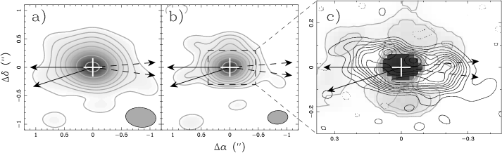
Figure 1: 350 GHz continuum maps toward the source. The cross marks the central star position. The solid and dashed arrows indicate the outflow axes on the blueshifted and redshifted sides, respectively. (a) and (b) show the maps at angular resolutions of $0^{\prime\prime}_{{}^{\textrm{.}}}53$$\times$$0^{\prime\prime}_{{}^{\textrm{.}}}35$ and $0^{\prime\prime}_{{}^{\textrm{.}}}36$$\times$$0^{\prime\prime}_{{}^{\textrm{.}}}24$, respectively. The contour levels are 8$\sigma(1-r^{n})/(1-r)$, where $r=1.55$, $n=1,2,3,..$, with $\sigma=3.7$ mJy Beam^-1 in (a) and $\sigma=2.4$ mJy Beam^-1 in (b). (c) shows the CLEAN component map of the continuum on top of the 23 GHz map of the H II shell adopted from Martin-Pintado et al. (1993). The contour levels start at 26 K with a step of 52 K. The compact emission peak at the center has a brightness temperature of $\sim$ 800 K.

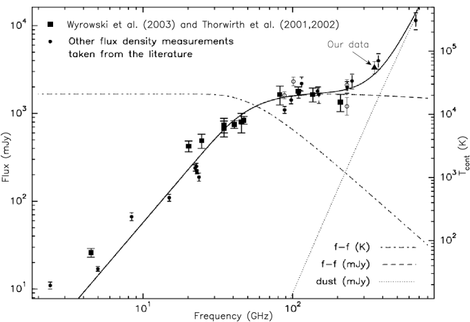
Figure 2: Spectral energy distribution of CRL 618. It is Figure 3 adopted from Wyrowski et al. (2003), and the fit in the figure was done by them. For other flux density measurements shown in the figure, please refer to that paper for the references. In their model, they assumed two components for the continuum, a free-free (f-f) emission from the H II region and a thermal dust emission from the envelope. The brightness temperature of the H II region was derived assuming a constant source size of $\sim$ $0^{\prime\prime}_{{}^{\textrm{.}}}22$. Previous OVRO (Owens Valley Radio Observatory) data from Sánchez Contreras & Sahai (2004) and Setal (04) are shown as open circles. Our SMA data at 350 GHz is also included and its flux density is consistent with the two-component model.

At 350 GHz, continuum emission is detected within $1^{\prime\prime}$ from the central star elongated in the east-west direction along the main outflow axis (Fig. 1a), with a total flux density of $\sim$ $3.3\pm$0.7 Jy. According to previous model for the spectral energy distribution (SED) of the source, the continuum emission at this frequency consists of two components: free-free emission from the H II region near the central star and thermal dust emission from the circumstellar envelope (see Fig. 2 and also Wyrowski et al., 2003). Note that for the flux density in the frequency between 80 and 360 GHz, Pardo et al. (2004, 2007) have found that the total flux density from the lines represents less than 3%-5% of the continuum and thus will not affect the analysis of the SED. Our flux density is consistent with the previous model, arising from the two components. Since the emission detected here is within $1^{\prime\prime}$ from the central star, the dust emission component here must be from the dense core of the circumstellar envelope, which has an outer radius of $\sim$ $1^{\prime\prime}_{{}^{\textrm{.}}}2$ (Setal, 04).

In order to distinguish the two components, we zoom into the emission peak at the center at higher resolution in Fig. 1b. However, the emission peak there is still not resolved. Since it is detected with a S/N ratio of more than 100, the structure there can be studied with the CLEAN component map shown in Figure 1c. In the map, a bright compact emission peak is seen at the center inside the H II shell detected at 23 GHz in the year of 1990 (Martin-Pintado et al., 1993). It has a brightness temperature of $\sim$ 800 K, but the actual value must be higher because it is unresolved. It has a flux density of $\sim$ 1.4$\pm 0.3$ Jy, roughly the same as that of free-free emission required to fit the SED of the continuum source (see Fig. 2). As a result, both the brightness temperature and flux density indicate that it traces the H II region. Note that the 23 GHz continuum map has been shifted by $\sim$ $0^{\prime\prime}_{{}^{\textrm{.}}}2$ to the north in order to match the center of the H II shell to the compact emission peak in our map. This position shift, if real, could be due to a proper motion of $\sim$ 40 km s^-1 to the north. As argued by Martin-Pintado et al. (1993), the H II region is a filled region. Since the H II region has a turnover frequency $<$ 100 GHz (see Fig. 2), the free-free emission at 350 GHz is optically thin. It appears as a peak at the center, indicating a presence of a dense inner part there. At 23 GHz, the H II region is optically thick. It appears as a shell probably because of an increase of electron temperature (Martin-Pintado et al., 1993) or an increase of density (Kwok & Bignell, 1984) there. At 350 GHz, the shell is optically thin and it is not detected here due to its not enough column density.

In the CLEAN component map, two faint emission peaks, one in the north and one in the south, are seen at a radius of $\sim$ $0^{\prime\prime}_{{}^{\textrm{.}}}14$ ($\sim$ 126 AU) from the central star roughly in the equatorial plane perpendicular to the outflow axes, surrounding the H II shell. The peak in the north also extends to the east and west surrounding the H II shell. These morphological relationships clearly indicate that these emissions trace the limb-brightened edges of the innermost part of the dense core around the H II shell. The two emission peaks may arise from a density enhancement in the dense core in the equatorial plane that helps confining the H II region into a bipolar morphology. The radius of the two emission peaks can set an upper limit for the current radius of the H II region in the equatorial plane. Less emission is seen in the outflow axes, suggesting that the dense core material there is cleared by the outflow.

Now it is clear that the extended emission in Figs. 1a and 1b traces the dense core. Since the free-free emission of the H II region has a flux density of $\sim$ 1.4$\pm 0.3$ Jy as discussed above, the thermal dust emission from the dense core has a flux density of $\sim$ 1.9$\pm 0.4$ Jy. In Figs. 1b, the emission in the east is resolved, extending to the northeast and southeast from the central star (Fig. 1b), likely tracing the dense core material around the outflow cavity walls. The emission is also seen extending $\sim$ $0^{\prime\prime}_{{}^{\textrm{.}}}6$ to the north from the central star, tracing the dense core that may have a density enhancement perpendicular to the outflow axes. However, no counterpart is seen extending to the south.

3.2 Molecular lines: Dense Core

3.2.1 Spectra

Figure 3 shows the spectra toward the inner region averaged over a circular region with a diameter of $0^{\prime\prime}_{{}^{\textrm{.}}}5$, from 342 to 346 GHz and from 354 to 358 GHz. The observed frequency has been converted to the rest frequency using the systemic velocity of $-21.5$ km s^-1 as found in Setal (04). Many molecular lines are detected, as listed in Table 1. Most of them are from HC₃N and its isotopologues, arising from rotational transitions at various vibrational states, as found at lower frequencies (Wyrowski et al., 2003; Pardo et al., 2007). As can be seen below, these molecules trace mainly the dense core. Most of their lines are isolated or almost isolated, so that their line peak brightness temperature $T_{B}^{p}$ and FWHM linewidth $\triangle v$ can be measured, as listed in Table 2, allowing us to derive the properties of the dense core. With an upper energy level ranging from $\sim$ 300 K up to 2000 K, these lines can be used to probe the properties of the dense core from the outer part down to the very inner part enclosing the H II region. Note that, sharp absorption dips are seen at $\sim$ $-$16 km s^-1 in strong molecular lines, e.g., CO (deepest at $-$15.8 km s^-1), CS ($-$15.8 km s^-1), HCO⁺ ($-$15.5 km s^-1), HCN $v=0$ ($-$15.8 km s^-1), and H¹³CN $v=0$ ($-$15.5 km s^-1), due to an absorption by the extended halo, which is cold and expanding at that velocity (Setal, 04). In this paper, we study the dense core mainly with HC₃N and its isotopologues. Other molecules trace mainly the outflow and will be studied in another paper.

3.2.2 Morphology

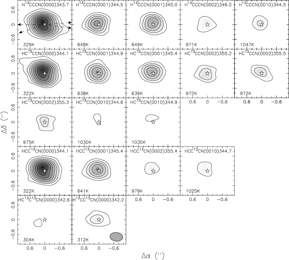
Figure 5: Same as that in Fig. 4 but for the lines of the HC₃N isotopologues. The contour levels are $A(1-r^{n})/(1-r)$, where $A=1$ Jy beam^-1 km s^-1, $r=1.2$, and $n=1,2,3,..$.

The integrated intensity maps of the isolated and almost isolated lines of HC₃N and its isotopologues are shown in Figures 4 & 5, respectively, in the order of increasing upper energy level of the lines. The figures show that for a given molecule, the structure of the emission shrinks closer to the central star as we go to the line with higher upper energy level, indicating that the temperature of the dense core increases toward the central star. In addition, comparing the two figures, we can also see that, for a given similar upper energy level, the lines of the isotopologues trace closer and thus warmer material than the HC₃N lines. This is because the isotopologues are less abundant and thus their lines are optically thinner. For the isotopologues with doubly substitutes of ¹²C with ¹³C, their abundances are very low, and their lines with low upper energy level mainly trace the dense core close to the central star (Fig. 5).

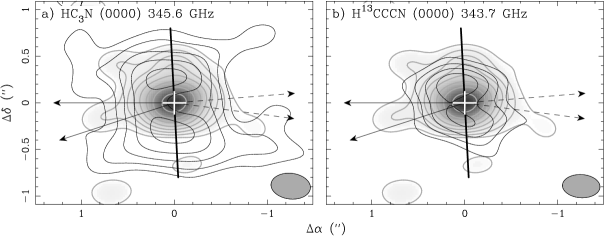
Figure 6: Integrated intensity maps of the (a) HC₃N (0000) and (b) H¹³CCCN (0000) lines on top of the continuum map shown in Fig. 1b, showing the structure of the dense core in the outer part. The cross marks the central star position and the arrows indicate the outflow axes. The solid line indicates the major axis of the dense core. The resolution is $\sim$ $0^{\prime\prime}_{{}^{\textrm{.}}}42$$\times$$0^{\prime\prime}_{{}^{\textrm{.}}}26$. The contour levels are $A(1-r^{n})/(1-r)$, with $n=1,2,3,..$. In (a) $A=2$ Jy beam^-1 km s^-1 and $r=1.4$. In (b) $A=1.2$ Jy beam^-1 km s^-1 and $r=1.3$.

For HC₃N and its singly ¹³C substituted isotopologues, the lines with the lowest upper energy level trace the outer part of the dense core that can be resolved in our observations. Figure 6 shows the maps for two of these lines, one in HC₃N and one in its isotopologue, H¹³CCCN, at a slightly higher angular resolution on top of the continuum map. Although the two lines have a similar upper energy level, the line of the isotopologue traces closer to the central star as discussed above. In these maps, two emission peaks, one in the north and one in the south of the central star, are seen surrounding the continuum emission peak, tracing the two limb-brightened edges of the dense core in the outer part. This two-emission peak structure was also seen in a lower excitation line of HC₃N before, and was used to suggest an equatorial density enhancement (mimicking a torus-like structure) in the dense core further out (Setal, 04).

The dense core is evacuated by the outflow lobes, with the emission around the outflow cavity walls extending to the northeast, southeast, northwest, and southwest, but with less emission along the outflow axes. In addition, the SE and SW outflow lobes evacuate more the southern part of the dense core, reducing more the emission there near the central star, as seen in H¹³CCCN. The major axis of the dense core, defined as the axis passing through the two emission peaks and the central star position, has a position angle of $\sim$ 3^∘, similar to that found by Setal (04), almost perpendicular to the east-west pair (i.e., the major pair) of the outflow lobes. Thus, the dense core is likely to be perpendicular to that pair of outflow lobes and is thus assumed to have an inclination angle of $\sim$ 30^∘ (Setal, 04), with the nearside tilted to the west and farside to the east. Note that the outer part of the dense core is expected to show a tilted ringlike structure in the maps, here we see more like a “C” structure because the emission is fainter in the western side of the central star, due to a self-absorption to be discussed later.

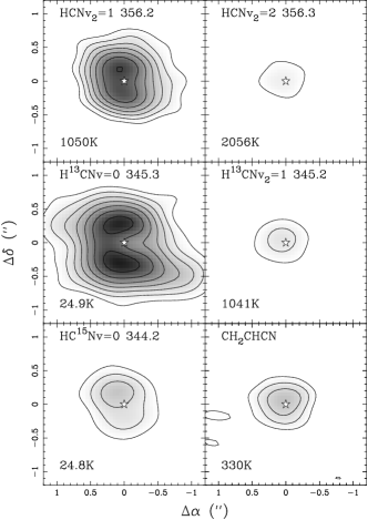
Figure 7: Same as that in Fig. 4 but for the lines of HCN and its isotopologues that trace the dense core. Also CH₂CHCN map is presented after summing over all the CH₂CHCN lines for a higher signal to noise ratio. The contour levels are $A(1-r^{n})/(1-r)$, where $A=2$ Jy beam^-1 km s^-1, $r=1.25$, and $n=1,2,3,..$.

Quite a few lines are also detected in HCN and its isotopologues (Fig. 3). Some of them also trace mainly the dense core and the maps of the isolated ones are shown in Figure 7. The HCN lines at the vibrational states $v_{2}=1$ and $2$ trace the dense core because of their high upper energy level and thus low number density at low temperature. The HCN line at ground vibrational state traces the outflow and is thus not shown here. The lines of H¹³CN $v=0$ and $v_{2}=1$, and HC¹⁵N $v=0$ trace the dense core due to their low abundances. Like that of HC₃N, the line with higher upper energy level traces the inner part of the dense core. We also detect many CH₂CHCN (Vinyl Cyanide) lines. A total of 120 lines of this molecule have been detected at lower frequency from 80 to 270 GHz by Pardo et al. (2007, see their Table 2). In our frequency ranges, there are 12 lines with the line strength $S_{ij}>96$ (a factor of 3 is included here for the spin-statistical weight of N). Here, 11 of them are detected and 1 at $\sim$ 356.247 GHz is lost in a strong HC₃N line (Fig. 3). These lines are weak, and thus we combine all of them to produce a map with a high signal to noise ratio, as shown in Figure 7. It is clear from the figure that these lines trace the innermost part of the dense core due to the low abundance of the molecule. This molecule could result from the interaction of C₂H₄ and CN, as discussed in Cernicharo (2004).

3.2.3 Kinematics

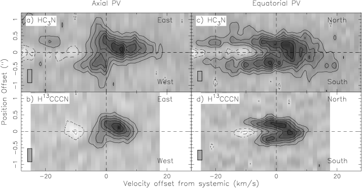
Figure 8: PV diagrams for the HC₃N (0000) and H¹³CCCN (0000) lines. (a) and (b) are the axial PV diagrams cut perpendicular to the dense core. (c) and (d) are the equatorial PV diagrams cut along the major axis of the dense core. The angular and velocity resolutions are shown in the lower left corner. The positive (negative) contours start from 16 ($-$16) K with a step of 16 ($-$16) K.

The kinematics of the dense core can be studied with the position-velocity (PV) diagrams using the same two lines that show the resolved structure of the dense core, as before. The axial PV diagrams, with the cut perpendicular to the dense core, show that the east side (or farside) is mainly redshifted and the west side (or nearside) is blueshifted (see Figs. 8a, b), in opposite to that seen for the outflow. Note that for HC₃N, the blueshifted emission with the velocity $\lesssim$ $-$10 km s^-1 should be ignored because it is contaminated by another weak HC₃N line centered at $-$20 km s^-1. This PV structure clearly supports that the core is expanding away from the central star. Negative contours are seen on the blueshifted side, due to an absorption of the continuum emission and the line emission by a cold layer on the nearside. Thus, the dense core appears fainter in the west of the central star, as seen above in Figure 6. The expansion velocity in each emission line is proportional to the maximum velocity, either redshifted or blueshifted. Since the blueshifted side is self-absorbed, the redshifted side is used, and the redshifted velocity is higher in the HC₃N line than in the H¹³CCCN line. Since the HC₃N line traces outer region than the H¹³CCCN line, this suggests that the expansion velocity increases with the distance from the central star. The equatorial PV diagrams, with the cut along the major axis of the dense core, show an incomplete ringlike PV structure due to the absorption on the blueshifted side (Figs. 8c, d). This ringlike PV structure indicates that for a given position offset from the central star, the blueshifted and redshifted emission are seen. This is expected because the dense core has a small inclination angle and it is thick enough for the cut to pass through both the farside and nearside of the dense core.

As mentioned above, the expansion velocity is found to increase with the distance from the central star. Here we can study quantitatively how fast the increase is, using the linewidth and the angular radius of the dense core seen in the lines of HC₃N and its isotopologues. We first measure the angular diameter and then divide it by two to obtain the angular radius. The angular diameter of the dense core in different line emission can be defined as the full extent in the major axis at the half maximum of the emission peak. It can be measured from those integrated maps (Figs. 4 & 5) that have enough signal to noise ratio, as listed in Table 2. Figure 9 shows the FWHM linewidth, $\triangle v$, versus the angular radius $r$ of the dense core. It shows that the linewidth and thus the expansion velocity increases roughly linearly with the angular radius. In this figure, we exclude the lines with the highest upper energy level, due to their low signal to noise ratio. Also, we exclude the zero vibrational line of HC₃N, which could be affected by the outflow lobes.

3.2.4 Physical Properties

Population diagram can be used to estimate the mean excitation temperature and the column density of HC₃N toward the inner part of the dense core. It is a diagram that plots the column density per statistical weight in the upper energy state in the optically thin limit, $N_{u}^{\textrm{\scriptsize thin}}/g_{u}$, versus the upper energy level $E_{u}$ of the HC₃N lines (Fig. 10). Here $N_{u}^{\textrm{\scriptsize thin}}=(8\pi k\nu^{2}/hc^{3}A_{ul})W$, where the integrated line intensity $W=\int T_{B}dv\approx 1.06T_{B}^{p}\cdot\triangle v$. The lines of the singly ¹³C substituted isotopologues can also be included in the diagram once their integrated line intensity is multiplied by the abundance ratio of HC₃N to the isotopologues. The abundance ratio has been found to be $\sim$ 10 (Wyrowski et al., 2003). This ratio is consistent with our observations because the line intensity of the isotopologues, after multiplied by this ratio, becomes aligned with that of the HC₃N lines in the diagram. The diagram shows almost a straight line if we exclude the data points for the HC₃N lines with $E_{u}/k<1000$ K. Those data points deviate significantly from the straight line because for those data points, (1) the lines become optically thick and (2) a significant fraction of the emission is outside the region that is used to derive the line intensity. The data points lie almost in a straight line, suggesting that the lines are mostly optically thin and arise from LTE material. Fitting the data with a straight line, we find that the mean excitation temperature and column density of the HC₃N molecules are $\sim$ 350 K and 9$\times 10^{16}$ cm^-2, respectively. The column density should be considered as a lower limit, because (1) the line of the isotopologues at the lowest upper energy level is not optically thin, showing an absorption dip in the blueshifted velocity as discussed above, and (2) the emission for line at lower upper energy is further away from the central star.

4 Model

In order to derive the properties of the dense core more accurately, we construct a radiative transfer model to calculate the free-free emission of the H II region, the thermal dust emission and molecular line emission of the dense core to compare with the observations.

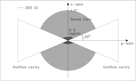
Figure 11: A schematic diagram for our simple model in the $yz$-plane, with $y$ to the west and $z$ to the north. The H II region (dark gray region) is ellipsoidal with a size of $0^{\prime\prime}_{{}^{\textrm{.}}}6$$\times$$0^{\prime\prime}_{{}^{\textrm{.}}}28$$\times$$0^{\prime\prime}_{{}^{\textrm{.}}}28$, and thus it has a radius of $0^{\prime\prime}_{{}^{\textrm{.}}}14$ in the $z$-axis and a radius of $0^{\prime\prime}_{{}^{\textrm{.}}}3$ in the $y$-axis. The dense core (light gray region) is spherical, with its outer radius set to $1^{\prime\prime}_{{}^{\textrm{.}}}2$ and its inner boundary set by the outer boundary of the ellipsoidal H II region. There are two outflow cavities, one in the east and one in the west, both with an half opening angle of 25^∘. In our model, the free-free emission is from the H II region, and both the dust and molecular emissions are from the dense core.

Figure 11 shows a schematic diagram for our model. As discussed in Sec. 3.1, the H II region is a filled region at the center elongated in the east-west direction. The radius of the H II region in the equatorial plane is uncertain and it might have grown to $\sim$ $0^{\prime\prime}_{{}^{\textrm{.}}}14$ as discussed. Thus, the H II region is assumed to be an ellipsoid with a size of $0^{\prime\prime}_{{}^{\textrm{.}}}6$$\times$$0^{\prime\prime}_{{}^{\textrm{.}}}28$$\times$$0^{\prime\prime}_{{}^{\textrm{.}}}28$ elongated in the east-west direction, which is an approximate representation of the size and morphology of the 23 GHz continuum map (Fig. 1). The inner radius of this H II region is unresolved and set to a small value of $0^{\prime\prime}_{{}^{\textrm{.}}}01$ (9 AU), which is more than 20 times smaller than our resolution and thus should not affect our model comparison. In order to produce the bright compact emission peak at the center, the electron density in the H II region is assumed to decrease with the radial distance from the central star, $r$, as follows

$$n_{e}=n_{e0}(\frac{r}{0^{\prime\prime}_{{}^{\textrm{.}}}05})^{-2}\;\textrm{cm}^{-3}$$ (1)

The electron temperature of the H II region is assumed to be constant at 15,000 K, in between that derived by Martin-Pintado et al. (1993) and Wyrowski et al. (2003). Note that the H II shell detected at 23 GHz could suggest an increase of electron temperature (Martin-Pintado et al., 1993) or density (Kwok & Bignell, 1984) in the outer part of the H II region. However, at 350 GHz, the shell is optically thin and it is not detected here because of its low column density. Therefore, its flux can be ignored as compared to that of the dense H II core at the center. As a result, the possible increase in the electron temperature or/and density is not included in our model.

The dense core is assumed to be spherical originally, with the inner radius set by the outer boundary of the H II region and the outer radius set to $1^{\prime\prime}_{{}^{\textrm{.}}}2$, as found in Setal (04). The dense core is excavated by the outflow lobes. For simplicity, we assume two outflow cavities, one in the east and one in the west, both with an half opening angle of 25^∘ (Figure 11), as judged from the HC₃N map in Fig 6a, which shows emission extending to the northeast, northwest, southeast, and southwest.

The dense core is dusty and molecular, producing both the thermal dust emission and molecular emission. For simplicity, the dust and molecular gas are assumed to have the same temperature. This temperature was first assumed to have a single power-law distribution as follows

$$T\propto r^{-p}\;\;\textrm{K}$$ (2)

We found that when $p=1.8$, this temperature distribution can roughly reproduce the low excitation lines in the outer part. However, it can not produce enough emission for the high excitation lines in the inner core, because the temperature there was too high. Therefore, the temperature is assumed to have the following two power-law distribution with a turning point at $r_{0}$

$$T(r)=\left\{\begin{array}[]{cl}T_{0}\big{(}\frac{r}{r_{0}}\big{)}^{-p_{i}}&\;\;\textrm{if}\;\;r<r_{0},\\ T_{0}\big{(}\frac{r}{r_{0}}\big{)}^{-p_{o}}&\;\;\textrm{if}\;\;r\geq r_{0}\end{array}\right.$$ (5)

with the power-law index $p_{i}<p_{o}$. In our model, the expansion velocity is assumed to increase linearly with the radius,

$$v_{\textrm{\scriptsize exp}}=v_{0}(\frac{r}{r_{0}})\;\;\textrm{km s${}^{-1}$}$$ (6)

as we discussed earlier. Note that, however, the dense core will have a maximum (i.e., terminal) expansion velocity, which is assumed to be equal to the expansion velocity of the extended halo or $\sim$ 16 km s^-1, as found earlier. The mass-loss rate in the dense core is assumed to be constant for simplicity, as in Fonfría et al. (2011). Thus, the number density of molecular hydrogen in the dense core becomes

$$n=n_{0}(\frac{r}{r_{0}})^{-3}\;\;\textrm{{cm}${}^{-3}$}$$ (7)

For the thermal dust emission in the dense core, the dust opacity per unit gas mass, $\kappa_{\nu}$, is assumed to be a free parameter in the order of 10^-2 cm² g^-1 at 350 GHz (Sahai et al., 2011). In the model, the molecules that trace the dense core are included. The outflow lines, e.g., CO, CS, HCO⁺, and HCN $v=0$, are excluded. The abundance of HC₃N is assumed to be $2\times 10^{-7}$ as found in Setal (04). The abundances of other molecular species are derived from our model by fitting the line profiles of each of these species.

Radiative transfer is used to calculate all the emissions with an assumption of LTE. The thermal linewidth and the linewidth due to a turbulence velocity of 2 km s^-1 are included. The systemic velocity is assumed to be -21.5 km s^-1. Also, we rotate our model counterclockwise by a P.A. of 3^∘ and tilt it with an inclination of 30^∘ to match the observations. The distance of the source is assumed to be 900 pc.

4.1 Model Results

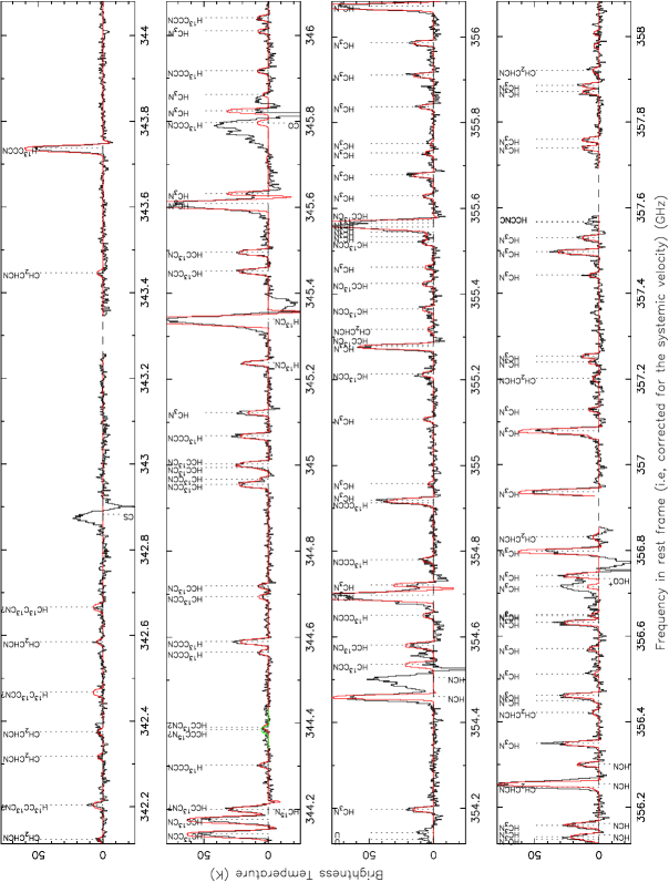
Figure 12: A fit to the spectra with our model. The black spectra are the same as those in Figure 3. Red spectra are derived from our model. The green spectrum shows the possible HCCC¹⁵N (0000) line at 344.3853481 GHz predicted from our model assuming an abundance ratio [HC₃N]/[HCCC¹⁵N]=150.

Figure 12 shows the fit of the spectra with our simple model. The parameters are listed in Table 3, and the profiles of the temperature, density, and velocity in the dense core are shown in Figure 13. In order to produce the observed flux density for the H II region, we obtain $n_{e0}=6.4\times 10^{6}$ cm^-3. For the inner, denser part of the H II region, the emission measure (EM) averaged over a radius of $0^{\prime\prime}_{{}^{\textrm{.}}}1$ is $\sim$ 4.2$\times 10^{10}$ cm^-6 pc, in agreement with that derived by Wyrowski et al. (2003), who assumed a radius of $\sim$ $0^{\prime\prime}_{{}^{\textrm{.}}}1$ for the H II region.

With the assumed abundance of HC₃N, we obtain the temperature, density, and velocity distributions of the dense core by fitting all the HC₃N lines that trace the dense core, including both the optically thin and optically thick lines. Then we derive the abundances of other molecular species by fitting their lines. The HC₃N isotopologues are much less abundant than HC₃N and their lines are mostly optically thin. For CH₂CHCN and HC¹⁵N, their lines are optically thin. For H¹³CN, the abundance is strongly constrained by the $v2=1$ J=4-3 line (at 345238.7103 MHz see Table 1), as this is optically thin ($\tau\sim 0.06$) in the region where the bulk of its emission arises (radii $<$ $0^{\prime\prime}_{{}^{\textrm{.}}}5$). For HCN, the abundance is strongly constrained by the v2 = 2 J=4-3 (at 356301.1780 MHz) and v2=1 J=4-3 (at 354460.4346 and 356255.5682 MHz) lines (see Table 1), as these have optical depths less than unity ($\tau\sim$ 0.08 and 0.70, respectively) in the region where the bulk of their emission arises (radii $<$ $0^{\prime\prime}_{{}^{\textrm{.}}}35$). Nonetheless, since our model assumes LTE, there could be uncertainty in our calculation of the abundances because of non-LTE effects.

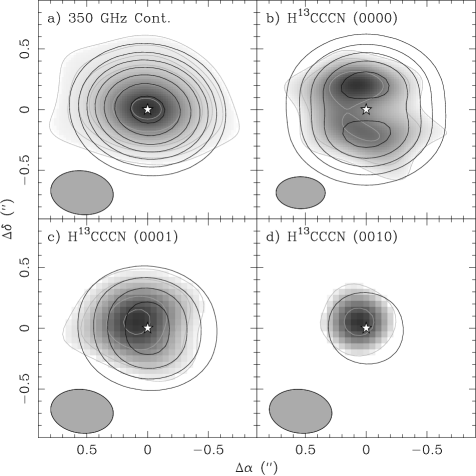
Figure 14: A comparison of the emission structure in the 350 GHz continuum and three H¹³CCCN lines at different vibrational states. The images with gray contours are from the observations, and the black contours are from our model. Panel (a) has the same contour levels as in Fig. 1a. The lowest contour is affected by the outflow and thus excluded. Panel (b) has the same contour levels as in Fig. 6b. Panels (c) and (d) have the same contour levels as in Fig. 5.

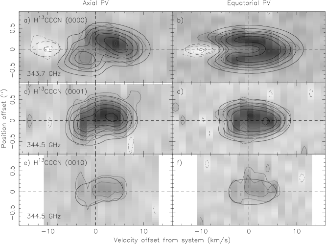
Figure 15: A comparison of the PV structure in the three H¹³CCCN lines at different vibrational states. The images with gray contours are from the observations, and the black contours are from our model. Panels (a) and (b) have the same contour levels as in Fig. 8b. In panels (c) to (f), the positive (negative) contours start from 6 ($-$6) K with a step of 6 ($-$6) K.

It is clear from Figure 12 that our model can roughly reproduce the line peak and linewidth for most of the lines that trace the dense core. As mentioned early, the outflow lines are excluded in the fitting. Since they are strong and broad, the lines that are close to them are significantly affected and thus can not be fitted well. In order to further check the reliability of our model, we also present the comparison of the synthetic and observed 350 GHz continuum maps as well as the maps for three emission lines. Since H¹³CCCN is mostly optically thin and bright, we choose three of its isolated lines at the different vibrational states that trace the different parts of the dense core. As can be seen from Figures 14 and 15, our model can also roughly reproduce the structures and the kinematics of the dense core in these emissions. Our model is symmetric and thus will not account for the asymmetric structure.

Nonetheless, there is still some minor discrepancy between our model and the observations. For the two bright HCN $v_{2}=1$ lines, although our model can roughly fit their line peak, it produces a linewidth smaller than the observed. This is probably because these two lines might have been affected by the outflows, as found in the line in the ground vibrational state of HCN. Also, for the three HC₃N isotopologues with doubly substitutes of ¹³C, we expect to see one line for each of them in our frequency ranges. However, the line of H¹³C¹³CCN at 342467.9204 MHz is not observed. Moreover, although we can roughly reproduce the peak of the lines for other two isotopologues, H¹³CC¹³CN and HC¹³C¹³CN, but the lines in our model are too broad. Since these lines are very weak, future observation at higher sensitivity will be needed to confirm our result.

In our model, since the density and temperature both decrease rapidly with the increasing radius, the line emissions are mainly arisen from the inner part of the dense core within $\sim$ $0^{\prime\prime}_{{}^{\textrm{.}}}7$ from the central star, as seen in the observations. In this part of the dense core, the expansion velocity increases from $\sim$ 3 km s^-1 to the maximum velocity of $\sim$ 16 km s^-1 at $r\sim$ $0^{\prime\prime}_{{}^{\textrm{.}}}7$ (630 AU). The outer part of the dense core does not change much the spectra, it only produces a deep absorption dip at $\sim$ $-16$ km s^-1 for the $v=0$ lines of HC¹⁵N, H¹³CN, and even HC₃N. This is because the expansion velocity there reaches and stays at the maximum velocity of $\sim$ 16 km s^-1.

The parameters in our model are consistent with what we estimated earlier. For instance, the mean column density of HC₃N averaged over a radius of $0^{\prime\prime}_{{}^{\textrm{.}}}5$ is $\sim 2\times 10^{17}$ cm^-2, only about 2 times the lower limit derived from the population diagram. The temperature averaged over a radius of $0^{\prime\prime}_{{}^{\textrm{.}}}5$ is $\sim$ 340 K, similar to the mean excitation temperature derived from the population diagram. The temperature power-law index in the outer part of the dense core is similar to that found in Setal (04) by fitting a low excitation line of HC₃N. The temperature power-law index in the inner part of the dense core is the same as that found in Wyrowski et al. (2003). The temperature within $r_{0}$ (i.e., $0^{\prime\prime}_{{}^{\textrm{.}}}22$) here is also consistent with that found by Fonfría et al. (2011). By fitting the infrared spectra of C₂H₂ and C₄H₂, they found that the temperature decreases from $\sim$ 600 K to 400 K from the innermost part of the dense core to $r_{0}$, similar to our model.

Previously, a sophisticated model has been proposed by Pardo et al. (Pardo et al., 2004, 2005; Pardo & Cernicharo, 2007; Pardo et al., 2007) to explain the various molecular emissions of CRL 618 observed with the IRAM 30m telescope in the frequency range from 80 to 276 GHz. The dense core here can be considered as a refined version of the slowly expanding envelope (SEE) in their model. In their model, the SEE has an outer radius of $1^{\prime\prime}_{{}^{\textrm{.}}}5$, slightly larger than that of the dense core. It has a temperature of 250-275 K, slightly lower than the mean temperature in the dense core. The expansion velocity field has a radial component ranging from 5 to 12 km s^-1, with a possible extra azimuthal component reaching 6 km s^-1 at $1^{\prime\prime}_{{}^{\textrm{.}}}5$, and is thus not much different from that in the dense core. The column density of HC₃N is $(2.0-3.5)\times 10^{17}$ cm^-2, also similar to that found in the dense core. In their model, the SEE is surrounded by a colder ($\sim$ 60 K) and outer (a radius from $1^{\prime\prime}_{{}^{\textrm{.}}}5$ to $2^{\prime\prime}_{{}^{\textrm{.}}}25$) circumstellar shell (CCS) created during the AGB phase, responsible for most of the rotational emission from HC₃N $\nu_{7}$ and $v=0$ and HC₅N $v=0$ (Pardo et al., 2005). In our model, there is no need for such an extended shell because our observations mostly probe the central region within $\sim$ $0^{\prime\prime}_{{}^{\textrm{.}}}7$ from the central star.

5 Discussion

Our model is very simple. Nonetheless, it already can produce a reasonable fit to the observations of the dense core. The abundance for each species is assumed to be constant, and no chemical effect is included. The dense core is assumed to be in LTE, which may not be the case near the central star because of a possible infrared pumping there. The different power-law index for the temperature in the inner part of the dense core could be related to this. The dense core is assumed to be spherical with 2 conical cavities. The actual dense core could have a density enhancement in the equatorial plane, as hinted in the continuum map and the map of the low excitation line of HC₃N (Setal, 04). This density enhancement in the equatorial plane, if real, could help confining the H II region into a bipolar morphology. Future model including these effects will be needed for a more detailed comparison.

The dense core could result from a recent heavy mass-loss episode that ends the AGB phase. The mass-loss rate in the dense core is $\dot{M}=4\pi r_{0}^{2}n_{0}v_{0}m_{\textrm{\scriptsize H}_{2}}\sim 1.15\times 10^{-3}$ M_⊙ yr^-1. It is $\gtrsim$ 2 orders of magnitude higher than the typical values of the AGB wind, indicating that the dense core could arise from an enhanced heavy mass loss that ends the AGB phase (Huggins, 2007). The total mass in the dense core is $\sim$ 0.47 $M_{\odot}$. If we divide this mass by the mass-loss rate, we will have a dynamical age of $\sim$ 400 yr for the dense core.

5.1 Nature of the H II region

At low frequency at 23 GHz, the H II region appears as a shell structure. Two scenarios were proposed to explain this shell structure. One scenario suggested that the H II region traces an ionized stellar wind photoionized by the central star (Martin-Pintado et al., 1988; Martin-Pintado et al., 1993). In this scenario, the H II region is a filled region and it appears as a shell due to a rapid increase of the electron temperature toward the edge. To have a filled region, the central star is required to be still in the mass-loss phase (Martin-Pintado et al., 1988). The other scenario suggested that the H II shell represents a nascent PN shell or a contact discontinuity as produced in an interacting-stellar winds model (Kwok & Bignell, 1984). In this model, a new fast wind generated in the PN phase interacts with the envelope formed by the stellar wind in the AGB phase. In both scenarios, a wind is required to be ejected from the central star.

Those two scenarios were proposed before the detections of fast moving optical collimated outflow lobes (Trammell & Goodrich, 2002; Sánchez Contreras et al., 2002) and fast moving massive molecular outflows (Setal, 04) in CRL 618. It is now believed that these fast moving phenomena are produced by a fast collimated post-AGB wind ejected after the AGB phase (or earlier at the end of the AGB phase) (see e.g. Lee & Sahai, 2003; Setal, 04). This fast wind interacts with the dense core, also producing a contact discontinuity at the interface. Thus, the H II shell may trace this contact discontinuity photoionized by the central star.

The compact H II peak at the center within the H II shell is seen for the first time in CRL 618. It may trace the post-AGB wind at the base photoionized by the central star. On the other hand, since the central star has become hot ($\sim$ 30,000 K) and luminous ($\sim$ 10⁴ $L_{\odot}$), a fast isotropic ionized wind may also be ejected from the central star by radiation pressure. Therefore, the compact H II peak may trace this fast wind as well. Further observations at higher resolutions are really needed to resolve it in order to check these possibilities

5.2 Dust Properties

As discussed in Sec. 3.1, at 350 GHz, the extended continuum emission traces the dust emission from the dense core and it has a flux density of $\sim$ 1.9$\pm 0.4$ Jy. Previously in single-dish observations, continuum emission was detected with a flux of $\sim$ 12$\pm 2.5$ Jy at 670 GHz (450 µm, see also Fig. 2) and 23$\pm 4$ Jy at 850 GHz (350 µm) (Knapp et al., 1993). As argued by the authors, the continuum emission at those two frequencies is highly dominated by the dust emission of the circumstellar envelope and thus the fluxes there can be considered as the upper limits for the dust emission in the dense core. Fitting to the fluxes at the 3 frequencies, we find the flux of the dense core $\propto\nu^{2.8\pm 0.2}$, which results in a dust emissivity index $\beta=0.8\pm 0.2$, as an upper limit. This value of $\beta$ is in good agreement with that derived by Knapp et al. (1993) for the circumstellar envelopes around five highly evolved stars, including CRL 618. A value of $\beta\lesssim 1$ has been used to imply a presence of large (mm-sized) grains in protoplanetary disks (Draine, 2006), as well as in torii and disks around post-AGB stars (Sahai et al., 2011). Thus, there could be large (mm-sized) grains in the dense core of CRL 618 as well down to $\sim$ 126 AU ($0^{\prime\prime}_{{}^{\textrm{.}}}14$) from the source.

In the dense core, the dust opacity per gas mass is found to be $\sim$ 0.022$\pm 0.004$ cm² g^-1 in our model. The gas-to-dust ratio is uncertain. It was found to be $\sim$ 63 with single-dish observations, averaged over both the extended halo and the dense core (Knapp et al., 1993). If we assume this ratio for the dense core, then the dust opacity per dust mass will be $\sim$ 1.4$\pm 0.3$ cm² g^-1, the same as that adopted to derive the mass of the disks and torii around the post-AGB stars (Sahai et al., 2011). Note that the gas-to-dust ratio could be a factor of 2 larger in the dense core as compared to that in the extended halo (Meixner et al., 2004), and so could be the dust opacity.

As discussed above, the dense core could result from a heavy mass loss at the end of the AGB phase. The mass loss (or wind) could be driven by radiation pressure of the stellar light on dust grains. For radiation driven wind, most of the acceleration is believed to take place in a very thin innermost part where the dust grains have sizes of up to a micrometer. Here in CRL 618, however, we see that the acceleration continues out to $0^{\prime\prime}_{{}^{\textrm{.}}}7$ (630 AU) even though the dust grains could have grown to mm sizes. Thus, further observations are needed to study the cause of this acceleration in the dense core.

5.3 Isotope Ratios

5.3.1 Carbon

Isotopic ratios can be used to constrain current nucleosynthesis models in evolved stars. Previously with the IRAM 30m single-dish observations, Pardo & Cernicharo (2007) found that the isotopic ratio of ¹²C/¹³C is 15 in the dense core [or slowly expanding envelope (SEE) in their model] and $\gtrsim 40$ in the extended halo [or circumstellar shell (CSS) in their model], using e.g., HC₃N, HCN, HNC, and their isotopologues in lower transition lines. Here, with the observations at higher angular resolutions in higher transition lines, the isotopic ratio of ¹²C/¹³C is found to be $\sim$ 10$\pm 3$, using HC₃N and its isotopologues. This value is the same as that found by Wyrowski et al. (2003) and similar to that found by Pardo & Cernicharo (2007) using the same species in lower transition lines. This is expected because this species is mainly present in the dense core (Setal, 04). The ratio is found to be $\sim$ 8$\pm 3$, using HCN and its isotopologues. Thus, the mean value of the ratio is $\sim$ 9$\pm 4$, similar to that found by Pardo & Cernicharo (2007) in the dense core using various molecules. Note that lower ¹²C/¹³C ratios have been seen before in C-rich PPN/PN, for instance, a value of $\sim$ 5 in Boomerang Nebula (PPN) (Sahai & Nyman, 1997), and a value of $\sim$ 3 in M1-16 [which is a very young multipolar PN with dense core (so very similar to CRL 618) and compact H II region] (Sahai et al., 1994).

Comparing to a recent extensive study by Milam et al. (2009) with ARO single-dish observations in CN, CO and their isotopologues, we find that our value is smaller than those found in the circumstellar envelopes around C-rich stars, which are $\sim$ 25-90, but it is in the lower limit of those found in the circumstellar envelopes around O-rich stars, which are $\sim$ 10-35. Note that in their study, the ratios are the values averaged over a large extent of the circumstellar envelopes including both the extended halos and dense cores. For CRL 618, they found a ratio of $\gtrsim$ 32, much larger than our value, probably due to a high ratio of $\gtrsim$ 40 found in the extended halo (Pardo & Cernicharo, 2007). In this case, high-resolution observations are really needed to derive the ratio in the dense core.

More recently, by modeling Herschel data of CO/¹³CO and HCN/H¹³CN lines in CRL 618, Wesson et al. (2010) found a ¹²C/¹³C ratio of 21, which is intermediate between the high value of $\gtrsim$ 40 and our low value of 9. The region they probed has a temperature of 70-230 K, and thus corresponds to our dense core in the middle part from $\sim$ $0^{\prime\prime}_{{}^{\textrm{.}}}3$ to $0^{\prime\prime}_{{}^{\textrm{.}}}6$. As a result, the ¹²C/¹³C ratio indeed appears to decrease (perhaps in a continuous manner) from $\gtrsim$ 40 in the extended halo to 9 in the inner part of the dense core, as argued by Pardo & Cernicharo (2007). The time scale for this change is short. In Pardo & Cernicharo (2007), the ratio of $\gtrsim$ 40 was obtained at a radius of $\sim$ $2^{\prime\prime}$. Our value is mostly from the inner part and can be assumed to be at a radius of $\sim$ $0^{\prime\prime}_{{}^{\textrm{.}}}3$. Assuming an expansion velocity of $\sim$ 16 km s^-1, then the time scale is only $\sim$ 450 yrs.

Our ¹²C/¹³C ratio in the dense core is much smaller than the solar value, which is $\sim$ 89. For an AGB star, the ¹²C/¹³C ratio is first expected to go down from the solar value due to the first dredge-up. This is because ¹³C, which is produced in CNO cycle during the RGB phase, is transported out to the envelope by the first dredge-up. Then when the 3rd dredge-up occurs adding fresh ¹²C to the envelope, the ¹²C/¹³C ratio starts going up again. When the envelope becomes C-rich, this ratio is expected to be $\gtrsim$ 35, which is what is seen in the extended halo in CRL 618. However, it is unclear how the ratio can decrease again after the envelope has become C-rich. As suggested by Pardo & Cernicharo (2007), one possibility is to have a late CNO cycling phase that follows He burning phase, as in Sakurai’s object (Asplund et al., 1999). Note that the ¹²C/¹³C equilibrium value from CNO cycling is $\sim$ 3.5 (Asplund et al., 1999).

5.3.2 Nitrogen

HC¹⁵N is clearly detected here in the dense core in J=4-3 line. It was also detected in J=1-0, 2-1, and 3-2 lines by Pardo et al. (2007) (see their electronic version of Fig. 5), although it was not listed in their Table 2. The isotopic ratio of ¹⁴N/¹⁵N in the dense core can thus be derived by dividing the abundance of HCN by that of HC¹⁵N and is found to be $\sim$ 130$\pm 40$. As discussed later, this value is low compared to those found in AGB stars (Wannier et al., 1991). It could be due to a possible underestimate of the HCN abundance in our model, considering that Thorwirth et al. (2003) has detected direct l-doubling transition lines of HCN (for which the line strengths are very low). We also derive an independent estimate of the ¹⁴N/¹⁵N ratio, $\sim$ 160$\pm$40, by multiplying the [H¹³CN]/[HC¹⁵N] ratio (16$\pm$4) by the ¹²C/¹³C ratio ($\sim$10, derived earlier from HC3N and its isotopologues). Therefore, the mean ratio of ¹⁴N/¹⁵N can be 150$\pm 50$. With this ratio, our model predicts a weak HCCC¹⁵N (0000) J=39-38 line at 344385.3481 MHz (see the green spectrum in Fig. 12), roughly consistent with the line emission feature tentatively detected there. However, such a feature could be alternatively identified with weak emission from the HCC¹³CN (0100)/(0003) J=38-37 (f component) transition (see the red spectrum in Fig. 12). Further work is needed to check this possible detection of the HCCC¹⁵N (0000) line.

In Pardo et al. (2007), CN and C₃N were not detected in the dense core (or their SEE), and neither were their ¹⁵N-isotopologues. Although HNC and HC₃N were also detected in the dense core, their ¹⁵N-isotopologues were not detected likely because of not enough sensitivity in their observations as discussed below. Since HNC lines are likely optically thick, we use HC¹⁵N lines in their observations to estimate the expected peak intensities for the H¹⁵NC lines. Assuming the abundance ratio of [HC¹⁵N]/[H¹⁵NC]=[HCN]/[HNC]= 10 (as found in the SEE by Pardo et al., 2007) and that the lines are optically thin, then the H¹⁵NC lines are expected to have a peak of $\sim$ 1 mK, 10 mK and 12 mK, respectively for J=1-0 (89 GHz), J=2-1 (178 GHz), and J=3-2 (267 GHz) lines. In their observations, the noise was $\sim$ 4 mK at 3mm (100 GHz), 8 mK at 2mm (150 GHz), 11 mK from 204 to 240 GHz, and 14 mK above 240 GHz, and thus those lines were lost in the noise. As for HCCC¹⁵N, here we only check if its (0000) lines can be detected because its higher vibrational lines are much weaker. In Pardo et al. (2007), the HC₃N (0000) lines have a peak of 0.4-0.6 K for those below 100 GHz and $\sim$ 1 K for those above 140 GHz. Assuming ¹⁴N/¹⁵N =150 (as derived above) and the lines are optically thin, then HCCC¹⁵N (0000) lines are expected to have a peak of $\sim$ 3 mK below 100 GHz and 7 mK above 140 GHz, and thus were also lost in the noise – more sensitive observations are needed.

Previously, using single-dish observations in HC₃N lines at lower frequencies, Wannier et al. (1991) derived a ¹⁵N$\times$¹²C/¹⁴N$\times$¹³C ratio of $<0.12$. Assuming a ¹²C/¹³C ratio of $\gtrsim$ 30, they estimated a ¹⁴N/¹⁵N ratio of $>250$. However, since the ¹²C/¹³C ratio in CRL618 decreases from $\gtrsim$ 40 in the extended halo to $\sim$ 9 in the dense core, the Wannier et al. lower limit on the ¹⁴N/¹⁵N ratio is $>$ 75 in the dense core, consistent with our derived value. Wannier et al. (1991) found the ¹⁴N/¹⁵N ratio to be $>$ 500 for their small sample of a few carbon-rich AGB stars and one PPN; Zhang et al. (2009) confirm this for AFGL 3068, finding ¹⁴N/¹⁵N$=$1099. CRL 618 appears to be different from these with its lower ¹⁴N/¹⁵N ratio. However, these studies use single-dish observations and their derived ratios are likely characteristic of the extended circumstellar envelopes in these objects, and not their dense central regions. High-resolution studies of these objects, like the one presented here, should be carried out to probe the latter.

Our value of ¹⁴N/¹⁵N is smaller than the solar value, which is $\sim$ 272. In current models of nucleosynthesis in the evolved stars, however, the CNO cycle is a cold CNO cycle that destroys ¹⁵N, resulting in a ¹⁴N/¹⁵N ratio always $\gtrsim$ 2000 (see, e.g., Palmerini et al., 2011). The only known way to produce abundant ¹⁵N is through a hot CNO cycle as in novae (Wiescher et al., 2010). However, it is unclear if the hot CNO cycle can really take place in the AGB stars at the end of the AGB phase. Also, chemical fractionation that can enhance the abundance of the isotopically-substituted species, is unlikely to be an effect at the high temperatures of the dense core, because it is important only at low temperatures (Terzieva & Herbst, 2000).

6 Conclusions

With the SMA, we have mapped the central region of CRL 618 in continuum and molecular lines at 350 GHz at $0^{\prime\prime}_{{}^{\textrm{.}}}3$ to $0^{\prime\prime}_{{}^{\textrm{.}}}5$ resolution. Most of the emission detected in our observations arises within a radius of $\sim$ 630 AU ($0^{\prime\prime}_{{}^{\textrm{.}}}7$) from the source. The main conclusions are the following:

• In the continuum, there are two components, (1) a compact emission at the center tracing the dense inner part of the H II region previously detected in 23 GHz continuum and it may trace a fast ionized wind at the base, and (2) an extended emission tracing the thermal dust emission from the dense core around the H II region. The dense core seems to have a density enhancement in the equatorial plane that can confine the H II region into a bipolar morphology. The dust emissivity index is estimated to be $0.8\pm 0.2$, suggesting that the dust grains in the dense core may have grown to mm size.

• The dense core is also detected in HC₃N, HCN, and their isotopologues, with higher excitation lines tracing closer to the source. It is also detected in CH₂CHCN toward the innermost part. The dense core detected here is the inner part of that seen before in a lower excitation line of HC₃N, and it could also have a density enhancement in the equatorial plane. The dense core is probably also excavated by the outflow lobes.

We have fitted a simple radiative transfer model to our observations in order to derive the kinematics, physical conditions, and the chemical abundances in the dense core. In this model, the H II region is ellipsoidal at the center. The dense core is spherical with the inner boundary set by the outer boundary of the H II region and the outer radius set to $1^{\prime\prime}_{{}^{\textrm{.}}}2$. It is dusty and molecular, producing both the thermal dust emission and molecular emission. Two outflow cavities are also included. This simple model can roughly fit the observations. The model results are the following:

• The dense core is expanding, with the velocity increasing roughly linearly from $\sim$ 3 km s^-1 in the innermost part to $\sim$ 16 km s^-1 at 630 AU. The mass-loss rate in the dense core is extremely high with a value of $\sim 1.15\times 10^{-3}$ M_⊙ yr^-1. The dense core has a mass of $\sim$ 0.47 $M_{\odot}{}$ and a dynamical age of $\sim$ 400 yrs. It could result from a recent enhanced heavy mass-loss episode that ends the AGB phase.

• The isotopic ratios of ¹²C/¹³C and ¹⁴N/¹⁵N are $\sim$ 9$\pm 4$ and $150\pm 50$, respectively, both smaller than the solar values. The ¹²C/¹³C ratio is also much smaller than that found in the extended halo, indicating that this ratio decreases toward the center, as argued before. It is not clear if current models of nucleosynthesis in evolved stars can produce our isotopic ratios in a C-rich star like that in CRL 618.

Table 1: Line Detections

Frequency	Species and	Rotational
(MHz)	Vibrational Statea	Transition J(QN)
342123.5509	CH2CHCN	J=36(12,24)-35(12,23)
342123.5509	CH2CHCN	J=36(12,25)-35(12,24)
342204.9747	H13CC13CN (0000)	J=39-38
342317.5544	CH2CHCN	J=36(5,32)-35(5,31)
342375.5639	CH2CHCN	J=36(5,31)-35(5,30)
342585.4708	CH2CHCN	J=36(4,33)-35(4,32)
342666.3834	HC13C13CN (0000)	J=38-37
342882.8503	CS	J= 7- 6
343446.5355	CH2CHCN	J=36(4,32)-35(4,31)
343737.3998	H13CCCN (0000)	J=39-38
344142.9833	HC13CCN (0000)	J=38-37
344176.1674	HCC13CN (0000)	J=38-37
344198.9411	HCC13CN (0100)/(0003)?	J=38-37
344200.1089	HC15N	J=4-3
344302.9375	H13CCCN (0010)	J=39-38
344385.3481	HCCC15N (0000)?	J=39-38
344390.9656	HCC13CN (0100)/(0003)?	J=38-37
344565.1094	H13CCCN (0010)	J=39-38
344590.0711	H13CCCN (0001)	J=39-38
344694.4713	HC13CCN (0010)	J=38-37
344719.4221	HCC13CN (0010)	J=38-37
344955.5335	HC13CCN (0001)	J=38-37
344967.3969	HC13CCN (0010)	J=38-37
344994.6742	HCC13CN (0010)	J=38-37
345003.2278	HCC13CN (0001)	J=38-37
345068.6323	H13CCCN (0001)	J=39-38
345122.5871	HC3N (1000)	J=38-37
345238.7103	H13CN $v_{2}=1$	J= 4- 3
345339.7694	H13CN	J= 4- 3
345451.7567	HC13CCN (0001)	J=38-37
345495.8736	HCC13CN (0001)	J=38-37
345609.0100	HC3N (0000)	J=38-37
345632.1266	HC3N (0100)/(0001)	J=38-37
345795.9899	CO	J= 3- 2
345797.0584	H13CCCN (0002)	J=39-38
345824.6653	HC3N (0100)/(0001)	J=38-37
345862.8068	HC3N (1002)/(0200)	J=38-37
345917.7699	H13CCCN (0002)	J=39-38
346010.5711	HC3N (1001)	J=38-37
346041.2173	H13CCCN (0002)	J=39-38
354127.5000	U
354143.5000	U
354197.5820	HC3N (1000)	J=39-38
354460.4346	HCN $v_{2}=1$	J= 4- 3
354505.4773	HCN	J= 4- 3
354535.7250	HC13CCN (0001)	J=39-38
354580.9970	HCC13CN (0001)	J=39-38
354650.5747	H13CCCN (0002)	J=40-39
354697.4631	HC3N (0000)	J=39-38
354721.1070	HC3N (0100)/(0001)	J=39-38
354780.4494	H13CCCN (0002)	J=40-39
354913.0924	H13CCCN (0002)	J=40-39
354918.6770	HC3N (0100)/(0001)	J=39-38
354957.7936	HC3N (1002)/(0200)	J=39-38
355108.4000	HC3N (1001)	J=39-38
355213.8330	HC13CCN (0002)	J=39-38
355277.5940	HC3N (0010)	J=39-38
355281.4277	HCC13CN (0002)	J=39-38
355317.9566	CH2CHCN	J=38(2,37)-37(2,36)
355365.4210	HC13CCN (0002)	J=39-38
355424.7668	HCC13CN (0002)	J=39-38
355463.0140	HC3N (0110)	J=39-38
355520.9620	HC13CCN (0002)	J=39-38
355533.6650	HC3N (0110)	J=39-38
355544.9810	HC3N (0110)	J=39-38
355556.5100	HC3N (0010)	J=39-38
355566.2540	HC3N (0001)	J=39-38
355572.7017	HCC13CN (0002)	J=39-38
355629.3710	HC3N (1001)	J=39-38
355678.1620	HC3N (0101)	J=39-38
355729.5000	HC3N (0110)	J=39-38
355751.3900	HC3N (0201)	J=39-38
355837.4410	HC3N (0020)	J=39-38
355910.9550	HC3N (0101)	J=39-38
355986.3120	HC3N (0101)	J=39-38
356072.4450	HC3N (0001)	J=39-38
356125.6170	HC3N (0020)	J=39-38
356131.7500	HC3N (0020)	J=39-38
356135.4600	HCN $v_{2}=2$	J= 4- 3
356158.0740	HC3N (0101)	J=39-38
356162.7700	HCN $v_{2}=2$	J= 4- 3
356247.4196	CH2CHCN	J=39(1,39)-38(1,38)
356255.5682	HCN $v_{2}=1$	J= 4- 3
356301.1780	HCN $v_{2}=2$	J= 4- 3
356349.7990	HC3N (0011)	J=39-38
356421.7169	CH2CHCN	J=39(0,39)-38(0,38)
356449.5064	HC3N (1002)/(0200)	J=39-38
356461.9430	HC3N (0011)	J=39-38
356511.7310	HC3N (0111)?	J=39-38
356570.8112	HC3N (1002)/(0200)	J=39-38
356632.0040	HC3N (0011)	J=39-38
356647.4090	HC3N (0111)?	J=39-38
356650.3550	HC3N (0111)?	J=39-38
356716.0590	HC3N (1002)/(0200)	J=39-38
356734.2230	HCO+	J= 4- 3
356742.1080	HC3N (0011)	J=39-38
356798.5018	HC3N (0002)	J=39-38
356832.0039	CH2CHCN	J=37(3,34)-36(3,33)
356937.1366	HC3N (0002)	J=39-38
357079.4470	HC3N (0002)	J=39-38
357129.0100	HC3N (0102)	J=39-38
357202.0855	CH2CHCN	J=37(2,35)-36(2,34)
357240.0820	HC3N (0102)	J=39-38
357254.0400	HC3N (0012)	J=39-38
357443.2270	HC3N (0102)	J=39-38
357497.4370	HC3N (0100)/(0001)	J=39-38
357530.2450	HC3N (0012)	J=39-38
357567.3400	HCCNC	J=36-35
357740.0520	HC3N (0012)	J=39-38
357759.7070	HC3N (0012)	J=39-38
357871.2740	HC3N (0012)	J=39-38
357885.9650	HC3N (0012)	J=39-38
357920.9088	CH2CHCN	J=38(1,37)-37(1,36)

Table 2: Line Information and Measurements of HC₃N, H¹³CCCN, HC¹³CCN, and HCC¹³CN

Molecule and	J	Frequency	Eu	$T_{B}^{p}$	$\triangle v$	Diameter
Vibrational State	Transition	(MHz)	(K)	(K)	(km s-1)	(”)
HC3N
(1000)	J=38-37	345122.5871	1590.042	25.0	8.0	0.59
(0000)i	J=38-37	345609.0100	323.493	77.0	17.0	1.12
(1001)	J=38-37	346010.5711	1907.628	7.0	6.5	–
(1000)	J=39-38	354197.5820	1607.041	22.0	8.0	0.57
(0000)i	J=39-38	354697.4631	340.516	77.0	17.5	1.09
(0100)/(0001)	J=39-38	354918.6770	1294.737	40.0	10.0	0.60
(1001)	J=39-38	355108.4000	1924.670	7.0	7.0	0.50
(0010)	J=39-38	355277.5940	1058.752	50.0	10.5	0.65
(0101)	J=39-38	355678.1620	1597.035	21.0	8.0	0.53
(0020)	J=39-38	355837.4410	1766.135	14.0	7.0	0.61
(0101)	J=39-38	355910.9550	1597.035	17.0	8.0	0.54
(0101)	J=39-38	355986.3120	1597.035	19.0	8.5	0.54
(0001)i	J=39-38	356072.4450	662.686	73.0	13.0	0.86
(0011)	J=39-38	356349.7990	1378.505	38.0	8.5	0.53
(0011)	J=39-38	356461.9430	1379.687	31.0	9.0	0.60
(1002)/(0200)	J=39-38	356570.8112	2246.276	3.5	8.0	–
(1002)/(0200)	J=39-38	356570.9650	2246.276	3.5	8.0	–
(0011)	J=39-38	356632.0040	1379.991	33.0	9.5	0.54
(0002)i	J=39-38	357079.4470	987.708	51.0	11.0	0.65
(0012)	J=39-38	357254.0400	1683.361	15.0	6.0	–
(0100)/(0001)	J=39-38	357497.4370	1298.070	38.0	8.5	0.58
(0012)	J=39-38	357530.2450	1683.361	15.5	9.0	0.48
(0012)	J=39-38	357740.0520	1683.361	13.0	9.0	0.60
(0012)	J=39-38	357759.7070	1683.361	13.5	8.0	0.60
(0012)	J=39-38	357871.2740	1683.361	12.5	8.5	0.54
(0012)	J=39-38	357885.9650	1683.361	15.0	6.5	–
H13CCCN
(0000)	J=39-38	343737.3998	329.992	55.0	11.0	0.76
(0010)	J=39-38	344565.1094	1047.903	8.5	7.5	0.52
(0001)	J=39-38	344590.0711	648.992	28.0	9.0	0.60
(0001)	J=39-38	345068.6323	649.453	28.0	8.0	0.61
(0002)	J=39-38	346041.2173	971.520	8.5	7.5	0.58
HC13CCN
(0000)	J=38-37	344142.9833	322.121	54.0	11.0	0.74
(0010)i	J=38-37	344694.4713	1030.321	5.0	7.5	–
(0001)	J=38-37	344955.5335	638.768	23.0	10.0	0.60
(0010)i	J=38-37	344967.3969	1030.577	6.0	5.0	–
(0001)	J=38-37	345451.7567	639.234	24.0	8.5	0.57
(0002)	J=39-38	355213.8330	972.521	13.0	8.5	0.58
(0002)	J=39-38	355365.4210	975.606	8.0	9.0	0.57
(0002)	J=39-38	355520.9620	975.684	10.0	7.5	0.46
HCC13CN
(0000)	J=38-37	344176.1674	322.152	51.0	11.5	0.74
(0010)	J=38-37	344719.4221	1025.870	8.0	7.0	–
(0001)	J=38-37	345495.8736	641.726	25.0	8.5	0.58
(0002)	J=39-38	355424.7668	979.687	8.5	6.0	–

Table 3: Model Parameters

Species	Abundance
HC3N	$2\pm 0.4\times 10^{-7}$
$\left.\begin{array}[]{l}\textrm{H${}^{13}$CCCN}\\ \textrm{HC${}^{13}$CCN}\\ \textrm{HCC${}^{13}$CN}\end{array}\right\}$	$2\pm 0.4\times 10^{-8}$
$\left.\begin{array}[]{l}\textrm{H${}^{13}$C${}^{13}$CCN}\\ \textrm{HC${}^{13}$C${}^{13}$CN}\\ \textrm{HCC${}^{13}$C${}^{13}$N}\end{array}\right\}$	$2\pm 0.4\times 10^{-9}$
CH2CHCN	$3\pm 0.6\times 10^{-8}$
HCN	$1.4\pm 0.3\times 10^{-7}$
H13CN	$1.8\pm 0.4\times 10^{-8}$
HC15N	$1.1\pm 0.3\times 10^{-9}$
Parameter	Value
$n_{e0}$	$6.4\pm 1.3\times 10^{6}$ cm-3
$r_{0}$	$0^{\prime\prime}_{{}^{\textrm{.}}}22$$\pm$$0^{\prime\prime}_{{}^{\textrm{.}}}04$
$T_{0}$	$440\pm 90$ K
$p_{i}$	$0.8\pm 0.2$
$p_{o}$	$1.8\pm 0.4$
$n_{0}$	$4.0\pm 0.8\times 10^{8}$ cm-3
$v_{0}$	4.9$\pm 0.5$ km s-1
$\kappa_{\nu}$	$0.022\pm 0.004$ cm2 g-1

Figure 3: Spectra toward the dense core, averaged over a circular region with a diameter of $0^{\prime\prime}_{{}^{\textrm{.}}}5$. Note that three small frequency intervals are empty, because of bad data and an incorrect correlator setup during the observations.

Figure 4: Integrated intensity maps of the HC₃N lines toward the dense core in the order of increasing upper energy level. The contour levels are $A(1-r^{n})/(1-r)$, where $A=1$ Jy beam^-1 km s^-1, $r=1.4$, and $n=1,2,3,..$. The star marks the central star position and the arrows indicate the outflow axes. In each panel, the upper right corner gives the vibrational state $(v_{4}v_{5}v_{6}v_{7})$ in parenthesis and rest frequency in GHz, and the lower left corner gives the upper energy level in K. The resolution is $0^{\prime\prime}_{{}^{\textrm{.}}}54$$\times$$0^{\prime\prime}_{{}^{\textrm{.}}}34$.

Figure 9: A plot of the FWHM linewidth versus the half width of the emitting size (or angular radius) of the dense core for the lines of HC₃N and its singly ¹³C substituted isotopologues. The solid line is a linear fit to the data.

Figure 10: Population diagram for HC₃N and its singly ¹³C substituted isotopologues. The line intensity of the isotopologues has been multiplied by a factor of 10. The solid line is a linear fit to the data. The HC₃N data points with an upper arrow are not optically thin and thus excluded from the fitting.

Figure 13: The temperature, density, and velocity distributions in the dense core in our best model.

References

- Asplund et al. (1999) Asplund, M., Lambert, D. L., Kipper, T., Pollacco, D., & Shetrone, M. D. 1999, A&A, 343, 507
- Balick & Frank (2002) Balick, B. & Frank, A. 2002, ARA&A, 40, 439
- Cernicharo et al. (2001a) Cernicharo, J., Heras, A. M., Pardo, J. R., et al. 2001, ApJ, 546, L127
- Cernicharo et al. (2001b) Cernicharo, J., Heras, A. M., Tielens, A. G. G. M., et al. 2001, ApJ, 546, L123
- Cernicharo (2004) Cernicharo, J. 2004, ApJ, 608, L41
- Draine (2006) Draine, B. T. 2006, ApJ, 636, 1114
- Fonfría et al. (2011) Fonfría, J. P., Cernicharo, J., Richter, M. J., & Lacy, J. H. 2011, ApJ, 728, 43
- Ho et al. (2004) Ho, P. T. P., Moran, J. M., & Lo, K. Y. 2004, ApJ, 616, L1
- Huggins (2007) Huggins, P. J. 2007, ApJ, 663, 342
- Knapp et al. (1993) Knapp, G. R., Sandell, G., & Robson, E. I. 1993, ApJS, 88, 173
- Kwok & Bignell (1984) Kwok, S., & Bignell, R. C. 1984, ApJ, 276, 544
- Lee et al. (2009) Lee, C.-F., Hsu, M.-C., & Sahai, R. 2009, ApJ, 696, 1630
- Lee & Sahai (2003) Lee, C.-F., & Sahai, R. 2003, ApJ, 586, 319
- Martin-Pintado et al. (1988) Martin-Pintado, J., Bujarrabal, V., Bachiller, R., Gomez-Gonzalez, J., & Planesas, P. 1988, A&A, 197, L15
- Martin-Pintado et al. (1993) Martin-Pintado, J., Gaume, R., Bachiller, R., & Johnson, K. 1993, ApJ, 419, 725
- Mbosei et al. (2000) Mbosei, L., Fayt, A., Dréan, P., & Cosléou, J. 2000, J. Mol. Structure, 517, 271
- Meixner et al. (2004) Meixner, M., Zalucha, A., Ueta, T., Fong, D., & Justtanont, K. 2004, ApJ, 614, 371
- Milam et al. (2009) Milam, S. N., Woolf, N. J., & Ziurys, L. M. 2009, ApJ, 690, 837
- Palmerini et al. (2011) Palmerini, S., La Cognata, M., Cristallo, S., & Busso, M. 2011, ApJ, 729, 3
- Pardo et al. (2004) Pardo, J. R., Cernicharo, J., Goicoechea, J. R., & Philips, T.G. 2004, ApJ, 615, 495
- Pardo et al. (2005) Pardo, J. R., Cernicharo, J., & Goicoechea, J. R. 2005, ApJ, 628, 275
- Pardo et al. (2007) Pardo, J. R., Cernicharo, J., Goicoechea, J. R., Guélin, M., & Asensio Ramos, A. 2007, ApJ, 661, 250
- Pardo & Cernicharo (2007) Pardo, J. R., & Cernicharo, J. 2007, ApJ, 654, 978
- Sahai et al. (1994) Sahai, R., Wootten, A., Schwarz, H. E., & Wild, W. 1994, ApJ, 428, 237
- Sahai & Nyman (1997) Sahai, R., & Nyman, L.-Å. 1997, ApJ, 487, L155
- Sahai et al. (2011) Sahai, R., Claussen, M. J., Schnee, S., Morris, M. R., & Sánchez Contreras, C. 2011, ApJ, 739, L3
- Sahai et al. (2007) Sahai, R., Morris, M., Sánchez Contreras, C., & Claussen, M. 2007, AJ, 134, 2200
- Sánchez Contreras & Sahai (2004) Sánchez Contreras, C., & Sahai, R. 2004, ApJ, 602, 960
- Setal (04) Sánchez Contreras, C., Bujarrabal, V., Castro-Carrizo, A., Alcolea, J., & Sargent, A. 2004, ApJ, 617, 1142 (Setal (04))
- Sánchez Contreras et al. (2002) Sánchez Contreras, C., Sahai, R., & Gil de Paz, A. 2002, ApJ, 578, 269
- Terzieva & Herbst (2000) Terzieva, R., & Herbst, E. 2000, MNRAS, 317, 563
- Thorwirth et al. (2003) Thorwirth, S., Wyrowski, F., Schilke, P., et al. 2003, ApJ, 586, 338
- Trammell & Goodrich (2002) Trammell, S. R., & Goodrich, R. W. 2002, ApJ, 579, 688
- Wannier et al. (1991) Wannier, P. G., Andersson, B.-G., Olofsson, H., Ukita, N., & Young, K. 1991, ApJ, 380, 593
- Wesson et al. (2010) Wesson, R., Cernicharo, J., Barlow, M. J., et al. 2010, A&A, 518, L144
- Wiescher et al. (2010) Wiescher, M., Görres, J., Uberseder, E., Imbriani, G., & Pignatari, M. 2010, Annu. Rev. Nucl. Part. Sci., 60, 381
- Wyrowski et al. (2003) Wyrowski, F., Schilke, P., Thorwirth, S., Menten, K. M., & Winnewisser, G. 2003, ApJ, 586, 344
- Zhang et al. (2009) Zhang, Y., Kwok, S., & Nakashima, J.-i. 2009, ApJ, 700, 1262