Scaling of heat flux and energy spectrum for “very large” Prandtl number convection

Abstract

Under the limit of infinite Prandtl number, we derive analytical expressions for the large-scale quantities, e.g., Péclet number Pe, Nusselt number Nu, and rms value of the temperature fluctuations $\theta_{\mathrm{rms}}$. We complement the analytical work with direct numerical simulations, and show that $\mathrm{Nu}\sim\mathrm{Ra}^{\gamma}$ with $\gamma\approx(0.30-0.32)$, $\mathrm{Pe}\sim\mathrm{Ra}^{\eta}$ with $\eta\approx(0.57-0.61)$, and $\theta_{\mathrm{rms}}\sim\mathrm{const}$. The Nusselt number is observed to be an intricate function of $\mathrm{Pe}$, $\theta_{\mathrm{rms}}$, and a correlation function between the vertical velocity and temperature. Using the scaling of large-scale fields, we show that the energy spectrum $E_{u}(k)\sim k^{-13/3}$, which is in a very good agreement with our numerical results. The entropy spectrum $E_{\theta}(k)$ however exhibits dual branches consisting of $k^{-2}$ and $k^{0}$ spectra; the $k^{-2}$ branch corresponds to the Fourier modes $\hat{\theta}(0,0,2n)$, which are approximately $-1/(2n\pi)$. The scaling relations for Prandtl number beyond $10^{2}$ match with those for infinite Prandtl number.

I Introduction

Thermal convection plays a significant role in many engineering applications, as well as in natural phenomena, e.g., mantle convection, atmospheric circulation, stellar convection etc. To simplify the complex nature of convective flow, it is customary to model the flow using a simpler setup called Rayleigh-Bénard convection (RBC), in which a thin horizontal layer of the fluid is heated from below and cooled from the top Ahlers et al. (2009a); Lohse and Xia (2010). The two non-dimensional control parameters that characterize RBC flow are the Rayleigh number Ra, which is a measure of buoyancy force, and the Prandtl number Pr, which is a ratio of kinematic viscosity and thermal diffusivity. The Nusselt number Nu is defined as the ratio of the total heat flux to conductive heat flux. Experiments and numerical simulations show that the RBC flow depends quite critically on the Prandtl number. In this paper we will describe the scaling of large-scale quantities and the energy spectrum for very large and infinite Prandtl number convection. Physics of large Prandtl number convection is important for understanding convection in Earth’s mantle, viscous oil, etc.

Kraichnan Kraichnan (1962) studied the scaling of Nusselt and Reynolds numbers theoretically using mixing-length theory, and deduced that $\mathrm{Nu}\sim\mathrm{Ra}^{1/3}$ for large Pr, $\mathrm{Nu}\sim(\mathrm{Pr}\mathrm{Ra})^{1/3}$ for small Pr, and $\mathrm{Nu}\sim 1$ for very small Pr. For RBC with very large Rayleigh numbers, called the “ultimate regime”, Kraichnan Kraichnan (1962) argued that $\mathrm{Nu}\propto(\mathrm{Ra}/\log(\mathrm{Ra}))^{1/2}$. Grossmann and Lohse Grossmann and Lohse (2000, 2001, 2002, 2004, 2011), Ahlers, et al. Ahlers et al. (2009a), and Stevens, et al. Stevens et al. (2013) modelled the scaling of Nusselt and Reynolds numbers using Shraiman and Siggia’s exact relations Shraiman and Siggia (1990) between the dissipation rates and the Nusselt number. For the dissipation rates, they considered the contributions from the bulk and boundary layers separately. They showed that the parameter space (Ra, Pr) is divided into four regimes: I for $U_{\mathrm{BL}},\theta_{\mathrm{BL}}$ dominated regime; II for $U_{\mathrm{bulk}},\theta_{\mathrm{BL}}$ dominated regime; III for $U_{\mathrm{BL}},\theta_{\mathrm{bulk}}$ dominated regime; and IV for $U_{\mathrm{bulk}},\theta_{\mathrm{bulk}}$ dominated regime; here $U_{\mathrm{BL}}$ and $\theta_{\mathrm{BL}}$ are respectively the rms value of the velocity and temperature fields in the boundary layer, while $U_{\mathrm{bulk}}$ and $\theta_{\mathrm{bulk}}$ are the corresponding quantities in the bulk. For the infinite or very large Prandtl number (kinematic viscosity $\gg$ thermal diffusivity), most of the flow is dominated by the viscous force. Grossmann and Lohse Grossmann and Lohse (2001) denote these regimes as I_∞ and III_∞ depending on the dominance of $\theta_{\mathrm{BL}}$ or $\theta_{\mathrm{bulk}}$ respectively. Throughout the paper we refer to the aforementioned scaling as “GL scaling”. In this paper, we report several numerical simulations for very large and infinite Prandtl number convection; these simulations fall in either I_∞ regime, or at the border of I_∞ and I_u. Also note that there are several mathematically rigorous bounds on the Nusselt number exponent. Whitehead and Doering Whitehead and Doering (2011) and Ierley, et al. Ierley et al. (2006) showed that $\mathrm{Nu}\leq c\mathrm{Ra}^{5/12}$ for free-slip boundary condition, while Constantin and Doering Constantin and Doering (1999) showed that $\mathrm{Nu}\leq c\mathrm{Ra}^{1/3}(1+\log(\mathrm{Ra}))^{2/3}$ in the limit of infinite Prandtl number.

A large number of experiments report the Nusselt number exponent within a range from 0.26 to 0.32 for Ra up to $10^{17}$ Castaing et al. (1989); Cioni et al. (1997); Glazier et al. (1999); Niemela et al. (2000); Ahlers and Xu (2001); Niemela and Sreenivasan (2003); Urban et al. (2012). However some experiments exhibit an increase in the exponent from 0.32 to 0.37, thus signalling a signature of ultimate regime Funfschilling et al. (2009); Ahlers et al. (2009b); He et al. (2012); Chavanne et al. (1997); Roche et al. (2001). The results from numerical simulations for small and medium Prandtl numbers and for Ra up to $10^{12}$ are consistent with the aforementioned experimental results Kerr (1996); Verzicco and Camussi (1999); Kerr and Herring (2000); Lohse and Toschi (2003); Verzicco and Sreenivasan (2008); Stevens et al. (2010a); Stevens et al. (2011); Verma et al. (2012); Verma et al. (2013a). However, in this paper we focus on very large and infinite Prandtl number convection.

There are only a small number of experiments that investigate large Prandtl number convection. Xia, et al. Xia et al. (2002) studied heat transport properties of 1-pentanol, triethylene glycol, dipropylene glycol, and water ($\mathrm{Pr}=4-1350$), and reported the Nusselt number exponent to be in a band of 0.281 to 0.307. Based on these observations, they claimed that $\mathrm{Nu}=0.14\mathrm{Ra}^{0.297}\mathrm{Pr}^{-0.03}$, thus suggesting a weak dependence of the Nusselt number on the Prandtl number in the large Prandtl number regime. Lam, et al. Lam et al. (2002) explored the dependence of Reynolds number ($\mathrm{Re}$) on Ra and Pr and showed that $\mathrm{Re}=0.84\mathrm{Ra}^{0.40}\mathrm{Pr}^{-0.86}$. Since the Péclet number $\mathrm{Pe}=\mathrm{Re}\mathrm{Pr}$, Lam, et al. Lam et al. (2002)’s work indicates a weak dependence of Pe on Pr.

Like experiments, numerical simulations of large Prandtl number convection are limited. Silano, et al. Silano et al. (2010) numerically analyzed the Nusselt number for a wide range of Prandtl numbers ($\mathrm{Pr}=10^{-1}$-$10^{4}$) and observed the Nusselt number exponents ranging from 2/7 for Pr = 1 to 0.31 for $\mathrm{Pr}=10^{3}$. In addition, they reported that for large Pr, $\mathrm{Pe}\sim\mathrm{Ra}^{1/2}$, and a constancy of thermal fluctuations with Ra. Roberts Roberts (1979) simulated two-dimensional RBC in the limit of $\mathrm{Pr}\rightarrow\infty$ and $\mathrm{Ra}\rightarrow\infty$ and reported that $\mathrm{Nu}\sim\mathrm{Ra}^{1/3}$ for the free-slip runs, and $\mathrm{Nu}\sim\mathrm{Ra}^{1/5}$ for the no-slip runs. Similar results have been reported by Hansen, et al. Hansen et al. (1990), Schmalzl, et al. Schmalzl et al. (2002), and Breuer, et al. Breuer et al. (2004) in two- and three-dimensional box simulations with free-slip boundary conditions. The aforementioned researchers also studied the structures of the flow and thickness of the boundary layers.

Another set of important quantities of interest in RBC are the energy spectrum and entropy spectrum ($|\hat{\theta}(\mathbf{k})|^{2}$). For intermediate Prandtl numbers, L’vov L’vov (1991) and L’vov and Falkovich L’vov and Falkovich (1992) predicted the Bolgiano-Obukhov scaling for small wavenumbers, but the Kolmogorov-Obukhov scaling for large wavenumbers. We will show in this paper that the spectra for the large and infinite Prandtl number convection differ from both these laws. Our arguments are similar to those of Batchelor Batchelor (1959) for small Prandtl number, except that the role of temperature and velocity is reversed in our work since the Prandtl number is large.

As discussed above, there are significant development in the understanding of large and infinite Prandtl number convection, especially from the GL scaling Grossmann and Lohse (2001). Still, many issues remain unresolved in this field. We address some of these issues using analytical approach and direct numerical simulation. Under the limit of infinite Prandtl number, we derive a linear relationship between the velocity and temperature fields, which enables us to derive interesting exact relations for the Péclet and Nusselt numbers. We also derive energy and entropy spectra analytically using the above relations, as well as the temperature equation. In addition, we also obtain analytic expressions for the thermal fluctuations, and viscous and thermal dissipation rates. The Nusselt number and thermal dissipation rates are intricately dependent on the Ra-dependent correlation between the vertical velocity and the temperature fluctuations. These relations provide valuable insights into large-Pr convective turbulence. It is important to note that our theoretical work are based on the dimensional and scaling analysis of the equations for the velocity and temperature fields. Our approach differs somewhat from the GL scaling, which is based on Shraiman and Siggia’s Shraiman and Siggia (1990) exact relation, and the scaling of the dissipation rates in the bulk and boundary layers.

To validate our analytical predictions, we perform direct numerical simulations of RBC flows for $\mathrm{Pr}=10^{2},10^{3},\infty$ and Rayleigh numbers varying from $10^{4}$ to $10^{8}$. Using the numerical data we compute scaling for the large-scale quantities like the Nusselt and Péclet numbers, the rms fluctuations of the temperature field, the viscous and thermal dissipation rates, and compare them with analytic predictions. We also compute energy and entropy spectra using the numerical data. We find that our numerical results are in good agreement with the analytical predictions, as well as with the GL scaling.

The structure of paper is as follows: In § II, we present the governing equations and analytical expressions for various large-scale quantities like the Nusselt and Péclet numbers, and the viscous and thermal dissipation rates. In § III we discuss the details of our numerical simulations. Scaling relations of Pe, Nu, and dissipation rates are discussed in § IV. In § V we derive energy and entropy spectra using the dynamical equations in the $\mathrm{Pr}=\infty$ limit, and complement them with the numerical results for infinite and large Prandtl number simulations. We conclude in § VI.

II Governing equations and analytic computations

The dynamical equations of RBC under Boussinesq approximations are

$$\frac{\partial\bf u}{\partial t}+(\bf u\cdot\nabla)\bf u = -\frac{\nabla p}{\rho_{0}}+\alpha g\theta\hat{z}+\nu\nabla^{2}\bf u,$$ (1)

$$\frac{\partial\theta}{\partial t}+(\bf u\cdot\nabla)\theta = \frac{\Delta}{d}u_{z}+\kappa\nabla^{2}\theta,$$ (2)

$$\nabla\cdot\bf u = 0,$$ (3)

where $\mathbf{u}=(u_{x},u_{y},u_{z})$ is the velocity field, $p$ and $\theta$ are respectively the deviations of pressure and temperature from the heat conduction state, $\rho_{0}$ is the mean density of fluid, $\alpha,\nu$, and $\kappa$ are respectively the thermal expansion coefficient, kinematic viscosity, and thermal diffusivity of fluid, $g$ is the acceleration due to gravity, $\hat{z}$ is the buoyancy direction, and $\Delta$ is the temperature difference between the two plates kept apart by a vertical distance $d$.

For large and infinite Prandtl number convection, it is customary to nondimensionalize the above set of equations using $\sqrt{\alpha g\Delta d/\mathrm{Pr}}$, $d$, and $\Delta$ as the velocity, length, and temperature scales respectively Silano et al. (2010), which yields

$$\frac{1}{\mathrm{Pr}}\left[\frac{\partial\bf u}{\partial t}+(\bf u\cdot\nabla)\bf u\right] = -\nabla\sigma+\theta\hat{z}+\frac{1}{\sqrt{\mathrm{Ra}}}\nabla^{2}\bf u,$$ (4)

$$\frac{\partial\theta}{\partial t}+(\bf u\cdot\nabla)\theta = u_{z}+\frac{1}{\sqrt{\mathrm{Ra}}}\nabla^{2}\theta,$$ (5)

$$\nabla\cdot\bf u = 0,$$ (6)

where $\mathrm{Ra}=\alpha g\Delta d^{3}/\nu\kappa$, $\mathrm{Pr}=\nu/\kappa$, and $\sigma=p/\mathrm{Pr}$ Silano et al. (2010); Schmalzl et al. (2002). Under the limit of $\mathrm{Pr}=\infty$, the momentum equation gets simplified to Breuer and Hansen (2009)

$$-\nabla\sigma+\theta\hat{z}+\frac{1}{\sqrt{\mathrm{Ra}}}\nabla^{2}{\bf u}=0.$$ (7)

The equations for the temperature field and the incompressibility condition remain unchanged. Note that the pressure term plays an important role in infinite Prandtl number convection, and it cannot be ignored. An easy inspection reveals that the $\nabla\cdot{\bf u}=0$ condition would be violated in the absence of the pressure term.

The momentum equation in a dimensional form is

$$-\nabla\sigma+\alpha g\theta\hat{z}+\nu\nabla^{2}{\bf u}=0.$$ (8)

The above equation is linear, hence analytically tractable. It is more convenient to analyze the above equation in Fourier space, which is

$$-i{\mathbf{k}}\hat{\sigma}(\mathbf{k})+\alpha g\hat{\theta}(\mathbf{k})\hat{z}-\nu k^{2}\hat{\mathbf{u}}(\mathbf{k}) = 0,$$ (9)

where ${\mathbf{k}}=(k_{x},k_{y},k_{z})$ is the wavenumber, and $\hat{f}(\mathbf{k})$ is the Fourier mode of the field $f$. Using the incompressible condition (${\mathbf{k}}\cdot\hat{\mathbf{u}}(\mathbf{k})=0$), we deduce that

$$\hat{\sigma}(\mathbf{k}) = -i\frac{k_{z}}{k^{2}}\alpha g\hat{\theta}(\mathbf{k}),$$ (10)

$$\hat{u}_{z}(\mathbf{k}) = \frac{\alpha g}{\nu}\frac{k_{\perp}^{2}}{k^{4}}\hat{\theta}(\mathbf{k}),$$ (11)

$$\hat{u}_{x,y}(\mathbf{k}) = -\frac{\alpha g}{\nu}\frac{k_{z}k_{x,y}}{k^{4}}\hat{\theta}(\mathbf{k}),$$ (12)

where $k_{\perp}^{2}=k_{x}^{2}+k_{y}^{2}$. The Fourier modes in general do not satisfy the boundary conditions at the plates. Yet, they capture the large-scale modes quite accurately since the energy of the convective flow is dominated by these modes. This feature becomes more significant for infinite Prandtl number since the amplitudes of the larger Fourier modes decrease steeply with the wavenumber ($\sim k^{-2}$), as evident from the aforementioned equations.

Using the above equations, we can derive the total kinetic energy as

$$E_{u}=\frac{1}{2}u^{2}=\frac{1}{2}\sum_{\mathbf{k}}|\hat{u}(\mathbf{k})|^{2}=\frac{1}{2}\left(\frac{\alpha g}{\nu}\right)^{2}\sum_{\mathbf{k}}|\hat{\theta}(\mathbf{k})|^{2}\frac{k_{\perp}^{2}}{k^{6}}.$$ (13)

The total energy is dominated by the large-scale flows. Therefore, the Péclet number Pe is

$$\mathrm{Pe}=\frac{U_{L}d}{\kappa}=\frac{d}{\kappa}\sqrt{2E_{u}}=\frac{\alpha gd}{\nu\kappa}\left(\sum_{\mathbf{k}}|\hat{\theta}(\mathbf{k})|^{2}\frac{k_{\perp}^{2}}{k^{6}}\right)^{1/2}.$$ (14)

In terms of nondimensional parameters

$$\mathrm{Pe}=\mathrm{Ra}\left(\sum_{\mathbf{k}}|\hat{\theta}(\mathbf{k})|^{2}\frac{k_{\perp}^{2}}{k^{6}}\frac{1}{d^{4}\Delta^{2}}\right)^{1/2}.$$ (15)

One of the generic features of thermal convection in a box is the finite amplitude of $\hat{\theta}(0,0,2n)$ Fourier modes for small $n$, e.g., $n=1,2,3$. Mishra and Verma Mishra and Verma (2010) showed using arguments based on energy transfers that

$$\hat{\theta}(0,0,2n)\approx-\frac{\Delta}{2n\pi}.$$ (16)

The $\hat{\theta}(0,0,2n)$ modes play an important role in determining the vertical profile of temperature. The temperature averaged over horizontal planes drops sharply near the plates (in the boundary layer), and it is approximately a constant in the bulk. We will show later in the paper that the temperature drop near the plates gets significant contributions from the $\hat{\theta}(0,0,2n)$ modes Verma et al. (2013a).

We will demonstrate later in the paper that the $\hat{\theta}(0,0,2n)$ modes dominate the temperature fluctuations for large and infinite Prandtl number convection. Thus,

$$\theta_{L}\approx\theta_{\mathrm{rms}}\approx\sqrt{2E_{\theta}}\approx\Delta,$$ (17)

where $E_{\theta}$ is defined as

$$E_{\theta}=\frac{1}{2}\theta^{2}=\frac{1}{2}\sum_{\mathbf{k}}|\hat{\theta}(\mathbf{k})|^{2}.$$ (18)

To quantify the contributions from other thermal modes, we define a residual temperature fluctuation $\theta_{\mathrm{res}}$ as

$$\theta_{\mathrm{res}}^{2}=\theta^{2}-\sum_{n}|\hat{\theta}(0,0,2n)|^{2}.$$ (19)

It is important to note that $\hat{u}_{z}(0,0,n)=0$ due to the absence of net mass flux across any horizontal cross-section in the box. As a result, the $\hat{\theta}(0,0,2n)$ modes do not contribute to the heat flux $H$, which is

$$H\propto\langle u_{z}\theta\rangle=\sum_{\mathbf{k}}(\hat{u}_{z}(\mathbf{k})\hat{\theta}^{*}(\mathbf{k})+\hat{u}^{*}_{z}(\mathbf{k})\hat{\theta}(\mathbf{k})),$$ (20)

where, $u_{z}^{*}$ and $\theta^{*}$ denote respectively the complex conjugate of the vertical velocity field and the temperature field. Thus, the heat flux gets contributions only from $\theta_{\mathrm{res}}$ fluctuations.

The viscous and thermal dissipation rates provide important information about the scaling of large-scale quantities Shraiman and Siggia (1990); Grossmann and Lohse (2000); Emran and Schumacher (2008, 2012). Shraiman and Siggia Shraiman and Siggia (1990) relate these dissipation rates to the Nusselt number using the following exact relationships:

$$\epsilon_{u} = \nu\langle|\nabla\times\mathbf{u}|^{2}\rangle=\frac{\nu^{3}}{d^{4}}\frac{(\mathrm{Nu}-1)\mathrm{Ra}}{\mathrm{Pr}^{2}},$$ (21)

$$\epsilon_{T} = \kappa\langle|\nabla T|^{2}\rangle=\kappa\frac{\Delta^{2}}{d^{2}}\mathrm{Nu},$$ (22)

where $T$ is the temperature field defined as $T=T_{\mathrm{conduction}}+\theta$. In the viscous regime, we use $\epsilon_{u}\propto\nu U_{L}^{2}/d^{2}$ and define a normalized viscous dissipation rate as

$$C_{\epsilon_{u}}=\frac{\epsilon_{u}}{\nu U_{L}^{2}/d^{2}}=\frac{(\mathrm{Nu}-1)\mathrm{Ra}}{\mathrm{Pe}^{2}}.$$ (23)

We define a normalized thermal dissipation rate as

$$C_{\epsilon_{T},1}=\frac{\epsilon_{T}}{\kappa\Delta^{2}/d^{2}}=\mathrm{Nu}.$$ (24)

Note that $\epsilon_{u}\propto U_{L}^{3}/d$ in turbulent regime, but this formula is not applicable for the large and infinite Prandtl number convection because of the laminar nature of the flow. The temperature equation however is fully nonlinear, hence $\epsilon_{T}\propto U_{L}\theta_{L}^{2}/d$ Grossmann and Lohse (2001); Emran and Schumacher (2008, 2012); Verma et al. (2013a). Therefore we define another normalized thermal dissipation rate as

$$C_{\epsilon_{T},2}=\frac{\epsilon_{T}}{U_{L}\theta_{L}^{2}/d}=\frac{\mathrm{Nu}}{\mathrm{Pe}}\left(\frac{\Delta}{\theta_{L}}\right)^{2}.$$ (25)

We will compute these dissipation rates using numerical data and use them for validation, as well as for the prediction of Nusselt number scaling.

III Numerical Method

We solve the nondimensionalized RBC equations [Eqs. (4, 5, 6)] numerically for both the free-slip and no-slip boundary conditions. We simulate free-slip RBC flow in a three-dimensional box of dimension $2\sqrt{2}:2\sqrt{2}:1$ using a pseudospectral code Tarang Verma et al. (2013b). On the top and bottom plates we employ free-slip and isothermal conditions for the velocity and temperature fields respectively. However, periodic boundary condition is employed on the lateral walls. Fourth-order Runge-Kutta (RK4) method is used for time advancement, and the 2/3 rule for dealiasing.

To complement the aforementioned free-slip numerical runs, we also simulate RBC flow under no-slip boundary condition in a two-dimensional box of aspect ratio one. We used the spectral element code NEK5000 Fischer (1997) for this purpose. Runs were performed in a box with $28\times 28$ spectral elements with 7th-order polynomials within each element, resulting in a $196^{2}$ effective grid points in the box. For the spectrum study however we used 15th-order polynomial, which yields $420^{2}$ effective grid points in the box. We will describe below that the two-dimensional no-slip and three-dimensional free-slip runs exhibit similar results for the large-scale quantities and energy spectrum.

We perform simulations for $\mathrm{Pr}=10^{2}$, $10^{3}$, $\infty$, and $\mathrm{Ra}$ in the range from $6\times 10^{4}$ to $1\times 10^{8}$. For such large Prandtl numbers, the kinematic viscosity is much larger than the thermal diffusion coefficient, consequently coherent thin plumes are generated in such flows Schmalzl et al. (2002); Hansen et al. (1990); Breuer et al. (2004); Stevens et al. (2010b). Fig. 1 illustrates the temperature isosurfaces of the flow structures for ($\mathrm{Pr}=10^{2},\mathrm{Ra}=10^{7}$), ($\mathrm{Pr}=10^{3},\mathrm{Ra}=6\times 10^{6}$), and ($\mathrm{Pr}=\infty,\mathrm{Ra}=6.6\times 10^{6}$). The figures demonstrate that the plumes become thinner and sharper with the increase of Prandtl number. Earth’s mantle that has very large Prandtl number ($\mathrm{Pr}\approx 10^{25}$) shows similar structures. A cross-sectional view of the flow pattern exhibits spoke like patterns, first shown by Busse and Whitehead Busse and Whitehead (1974) in their experiments with silicone oil. Also, $k_{\mathrm{max}}\eta_{u}\gtrsim 1$ and $k_{\mathrm{max}}\eta_{\theta}\gtrsim 1$ for all of our simulation runs; here $\eta_{u}=(\nu^{3}/\epsilon_{u})^{1/4}$ and $\eta_{\theta}=(\kappa^{3}/\epsilon_{u})^{1/4}$ are the Kolmogorov length and Batchelor length for the velocity and temperature fields respectively. Thus our simulations are numerically well resolved.

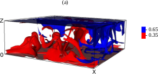
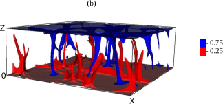
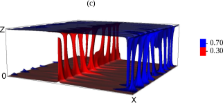
Figure 1: (Color online) Temperature isosurfaces for (a) $\mathrm{Pr}=10^{2}$ and $\mathrm{Ra}=10^{7}$, (b) $\mathrm{Pr}=10^{3}$ and $\mathrm{Ra}=6\times 10^{6}$, and (c) $\mathrm{Pr}=\infty$ and $\mathrm{Ra}=6.6\times 10^{6}$. The red structures represent hot plumes, and blue ones represent cold plumes. The large-scale structures get sharper with the increase of Pr.

Table 1: Details of numerical simulations performed for free-slip boundary condition. The table contains Péclet number Pe, Nusselt number Nu; the normalized viscous dissipation rate: numerically computed $C_{\epsilon_{u}}^{\mathrm{comp.}}=\epsilon_{u}/(\nu U^{2}_{L}/d^{2})$, and estimated $C_{\epsilon_{u}}^{\mathrm{est.}}=(\mathrm{Nu}-1)\mathrm{Ra}/\mathrm{Pe}^{2}$; the normalized thermal dissipation rates: numerically computed $C_{\epsilon_{{}_{T}},1}^{\mathrm{comp.}}=\epsilon_{{}_{T}}/(\kappa\Delta^{2}/d^{2})$, $C_{\epsilon_{{}_{T}},2}^{\mathrm{comp.}}=\epsilon_{{}_{T}}/(U_{L}\theta^{2}_{L}/d)$, and estimated $C_{\epsilon_{{}_{T}},2}^{\mathrm{est.}}=(\mathrm{Nu}/\mathrm{Pe})(\Delta/\theta_{L})^{2}$. It also lists globally averaged $k_{\mathrm{max}}\eta_{u}$ and $k_{\mathrm{max}}\eta_{\theta}$, which are $\gtrapprox 1$ for all the cases.

Pr	Ra	Grid	Nu	Pe	$C_{\epsilon_{u}}^{\mathrm{comp.}}$	$C_{\epsilon_{u}}^{\mathrm{est.}}$	$C_{\epsilon_{{}_{T}},1}^{\mathrm{comp.}}$	$C_{\epsilon_{{}_{T}},2}^{\mathrm{comp.}}$	$C_{\epsilon_{{}_{T}},2}^{\mathrm{est.}}$	$k_{\mathrm{max}}\eta_{u}$	$k_{\mathrm{max}}\eta_{\theta}$
$10^{2}$	$1.0\times 10^{5}$	$256^{3}$	9.8	$1.98\times 10^{2}$	22.3	22.3	9.8	0.60	0.60	61.4	1.9
$10^{2}$	$2.0\times 10^{5}$	$256^{3}$	11.2	$2.92\times 10^{2}$	24.0	23.9	11.2	0.47	0.46	50.0	1.6
$10^{2}$	$6.5\times 10^{5}$	$256^{3}$	17.3	$6.15\times 10^{2}$	28.6	28.3	17.5	0.36	0.34	32.0	1.0
$10^{2}$	$2.0\times 10^{6}$	$512^{3}$	24.1	$1.20\times 10^{3}$	32.1	32.2	24.1	0.25	0.24	45.7	1.4
$10^{2}$	$5.0\times 10^{6}$	$512^{3}$	31.0	$1.96\times 10^{3}$	39.5	39.1	30.9	0.19	0.19	33.9	1.1
$10^{2}$	$1.0\times 10^{7}$	$1024^{3}$	38.1	$2.92\times 10^{3}$	43.7	43.4	38.2	0.16	0.16	54.3	1.7
$10^{3}$	$6.5\times 10^{4}$	$256^{3}$	8.6	$1.53\times 10^{2}$	21.4	21.4	8.6	0.69	0.68	223	1.3
$10^{3}$	$1.0\times 10^{5}$	$256^{3}$	9.8	$1.98\times 10^{2}$	22.3	22.3	9.8	0.60	0.60	194	1.1
$10^{3}$	$2.0\times 10^{5}$	$512^{3}$	12.1	$3.01\times 10^{2}$	23.9	23.9	12.1	0.48	0.48	309	1.7
$10^{3}$	$3.2\times 10^{5}$	$512^{3}$	14.1	$3.98\times 10^{2}$	27.2	27.1	14.1	0.42	0.43	261	1.5
$10^{3}$	$2.0\times 10^{6}$	$1024^{3}$	24.3	$1.10\times 10^{3}$	38.7	38.3	24.3	0.26	0.26	277	1.6
$10^{3}$	$6.0\times 10^{6}$	$1024^{3}$	34.2	$2.13\times 10^{3}$	43.4	43.7	34.2	0.19	0.19	200	1.1
$\infty$	$7.0\times 10^{4}$	$128^{3}$	8.8	$1.59\times 10^{2}$	21.4	21.6	8.8	0.67	0.68	$\infty$	1.7
$\infty$	$1.9\times 10^{5}$	$128^{3}$	12.1	$3.02\times 10^{2}$	23.9	24.0	12.0	0.48	0.49	$\infty$	2.4
$\infty$	$3.2\times 10^{5}$	$128^{3}$	14.1	$4.14\times 10^{2}$	25.1	25.1	14.1	0.41	0.42	$\infty$	2.0
$\infty$	$6.5\times 10^{5}$	$128^{3}$	17.4	$6.36\times 10^{2}$	26.7	26.7	17.4	0.33	0.34	$\infty$	1.6
$\infty$	$3.9\times 10^{6}$	$256^{3}$	30.3	$1.95\times 10^{3}$	30.3	30.4	30.3	0.19	0.19	$\infty$	1.8
$\infty$	$6.5\times 10^{6}$	$256^{3}$	36.1	$2.70\times 10^{3}$	33.5	31.8	36.0	0.16	0.16	$\infty$	1.5
$\infty$	$9.8\times 10^{6}$	$256^{3}$	41.2	$3.34\times 10^{3}$	35.8	35.6	41.1	0.15	0.15	$\infty$	1.3
$\infty$	$1.9\times 10^{7}$	$256^{3}$	51.2	$5.20\times 10^{3}$	36.8	36.6	51.2	0.12	0.12	$\infty$	1.1
$\infty$	$1.0\times 10^{8}$	$512^{3}$	87.5	$1.38\times 10^{4}$	45.6	45.3	87.2	0.07	0.07	$\infty$	1.3

Table 2: Details of RBC simulations with no-slip boundary condition for a two-dimensional box of aspect ratio one.

Pr	Ra	Grid	Nu	Pe
$10^{2}$	$1\times 10^{4}$	$196^{2}$	2.2	$1.43\times 10^{1}$
$10^{2}$	$1\times 10^{5}$	$196^{2}$	3.9	$5.73\times 10^{1}$
$10^{2}$	$1\times 10^{6}$	$196^{2}$	7.1	$1.93\times 10^{2}$
$10^{2}$	$1\times 10^{7}$	$420^{2}$	14.4	$7.55\times 10^{2}$
$10^{2}$	$5\times 10^{7}$	$196^{2}$	22.6	$1.99\times 10^{3}$

We compute various global quantities (e.g., $\theta_{L}$, Péclet and Nusselt numbers), and energy and entropy spectra using the numerical data generated by our simulations. These quantities are averaged over 200-300 eddy turnover time after the flow has reached a steady state. Note that the system takes around a thermal diffusive time to reach a steady state. For better statistical averaging, the Nusselt number is computed by averaging the heat flux over the box volume. For all our runs, the number of grid points in the thermal boundary layers are greater than 5 to 6, which is consistent with the Grötzbach criteria Grötzbach (1983). For example, for Pr = $\infty$ and Ra = $10^{8}$, the thermal boundary layers at both the plates contain 10 points.

Table 1 exhibits details of our free-slip numerical simulations. In the table, we list the normalized dissipation rates computed using the numerical data and compare them with the ones derived using the exact relations (using the Nusselt number). The estimated values are in very good agreement with the numerically computed ones, thus validating our numerical simulations. We however remark that the viscous and thermal dissipation rates exhibit temporal and spatial variability, as shown by many researchers. For example, Emran and Schumacher Emran and Schumacher (2008, 2012) performed a detailed numerical analysis of the thermal dissipation rate $\epsilon_{T}$ and showed that the scaling of $\epsilon_{T}$ in boundary layer and in bulk are different.

The details of our no-slip runs are exhibited in Table 2. We also ensured grid-independence of our numerical program by performing simulations on grids with higher and lower resolutions, and comparing our results. The global quantities like Péclet and Nusselt numbers were found to be within 1-2% for these simulation.

In the next section we will describe the scaling of large-scale quantities derived using the numerical data.

IV Scaling of large-scale quantities

In this section we report average values of the Péclet and Nusselt numbers, as well as that of the temperature fluctuations and dissipation rates, for various Prandtl and Rayleigh numbers. These values are compared with the analytical predictions.

IV.1 Temperature fluctuations

For large Prandtl number convection, Silano, et al. Silano et al. (2010) showed that the temperature fluctuations are independent of Ra and Pr. Here we analyze this issue in more detail. As discussed in the previous section, $\hat{\theta}(0,0,2n)$ modes play an important role in turbulent convection. We compute $\hat{\theta}(0,0,2n)$ modes for small $n$ using the numerical data of our simulation. These values, exhibited in Table 3 for some typical parameters, are in good agreement with the predictions of Mishra and Verma Mishra and Verma (2010) that $\hat{\theta}(0,0,2n)\approx-\Delta/(2n\pi)$. In Fig. 2 we plot the averaged temperature profile $\bar{T}(z)$, as well as $1-z+\sum_{n}2\hat{\theta}(0,0,2n)\sin(2\pi nz)$ for $n=1,2,4$ and 10 (note that $T_{\mathrm{conduction}}=1-z$). The figure demonstrates that the $\bar{T}(z)$ is well approximated by $1-z+\sum_{n=0}^{10}2\hat{\theta}(0,0,2n)\sin(2\pi nz)$. Hence we conclude that the $\hat{\theta}(0,0,2n)$ modes contribute significantly to $\bar{T}(z)$.

Table 3: Numerically computed values of the Fourier modes $\hat{\theta}(0,0,2)$, $\hat{\theta}(0,0,4)$, $\hat{\theta}(0,0,6)$, and $\hat{\theta}(0,0,8)$ for $\mathrm{Pr}=10^{2},10^{3},$ and $\infty$. The values obtained from our simulation are in good agreement with Mishra and Verma’s Mishra and Verma (2010) theoretical prediction that $\hat{\theta}(0,0,2n)$ $\approx-1/2\pi n$ (the last row of the table).

Pr	Ra	$\hat{\theta}(0,0,2)$	$\hat{\theta}(0,0,4)$	$\hat{\theta}(0,0,6)$	$\hat{\theta}(0,0,8)$
$10^{2}$	$1\times 10^{7}$	-0.16	-0.081	-0.054	-0.040
$10^{3}$	$6\times 10^{6}$	-0.16	-0.082	-0.055	-0.040
$\infty$	$1\times 10^{8}$	-0.16	-0.080	-0.054	-0.041
-	$-1/2\pi n$	-0.16	-0.080	-0.053	-0.039

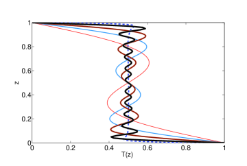
Figure 2: (Color online) Averaged temperature $T(z)$ (dashed blue curve) as a function of $z$ for $\mathrm{Pr}=\infty$ and $\mathrm{Ra}=10^{8}$. The mean temperature remains almost a constant in the bulk, and it displays a sharp gradient near the top and bottom plates. The red, sky blue, brown, and black curves (curves with increasing thickness) represent $T_{c}+\sum_{n}2\hat{\theta}(0,0,2n)\sin(2\pi nz)$ for $n=1,2,4$, and 10 respectively; here $T_{c}=1-z$ is the conduction profile. The curve for $n=10$ matches quite well with $T(z)$.

We also compute the residual temperature fluctuations $\theta_{\mathrm{res}}$ defined using Eq.(19), and observe that

$$\theta_{\mathrm{res}}=a_{1}\Delta\mathrm{Ra}^{-\delta},$$ (26)

as shown in Fig. 3. We deduce that $\theta_{\mathrm{res}}/\Delta=(0.59\pm 0.08)\mathrm{Ra}^{-0.15\pm 0.01}$ for $\mathrm{Pr}=\infty$, $\theta_{\mathrm{res}}/\Delta=(0.49\pm 0.02)\mathrm{Ra}^{-0.13\pm 0.01}$ for $\mathrm{Pr}=10^{2}$, and $\theta_{\mathrm{res}}/\Delta=(0.56\pm 0.04)\mathrm{Ra}^{-0.14\pm 0.01}$ for $\mathrm{Pr}=10^{3}$. Thus, the scaling exponents as well as the prefactors of $\theta_{\mathrm{res}}$ for various Prandtl numbers are nearly same for $\mathrm{Pr}\geq 10^{2}$.

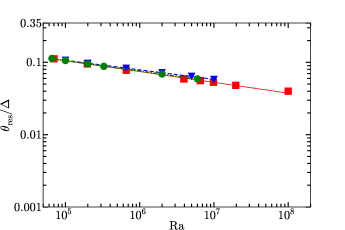
Figure 3: (Color online) Normalized residual temperature fluctuation ($\theta_{\mathrm{res}}/\Delta$) as a function of Ra for free-slip runs. The data for $\mathrm{Pr}=\infty$ (red squares), $\mathrm{Pr}=10^{2}$ (blue down-pointing triangles), and $\mathrm{Pr}=10^{3}$ (green circles) collapse to a single function $\theta_{\mathrm{res}}\approx a_{1}\Delta\mathrm{Ra}^{-\delta}$. The prefactors and exponents for the three runs are approximately equal.

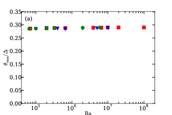
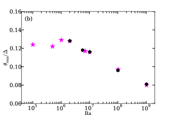
Figure 4: (Color online) Plots of normalized root mean square thermal fluctuations ($\theta_{\mathrm{rms}}/\Delta$) vs. Ra: (a) Upper panel: for our 3-d free-slip runs with $\mathrm{Pr}=\infty$ (red squares), $\mathrm{Pr}=10^{2}$ (blue down-pointing triangles), and $\mathrm{Pr}=10^{3}$ (green circles); (b) Bottom panel: for the 3-d no-slip simulations by Silano, et al. Silano et al. (2010) with $\mathrm{Pr}=10^{3}$ (pink stars), and $\mathrm{Pr}=10^{2}$ (black hexagons). $\theta_{\mathrm{rms}}/\Delta$ is an approximate constant for the free-slip boundary condition. For the no-slip boundaries Silano et al. (2010), $\theta_{\mathrm{rms}}/\Delta$ is a constant for lower $\mathrm{Ra}$, and it is a weakly decreasing function of $\mathrm{Ra}$ for larger $\mathrm{Ra}$.

For our large Pr convection with free-slip boundary condition, we observe that $\theta_{\mathrm{res}}\ll\hat{\theta}(0,0,2)$. Consequently, the rms fluctuation of $\theta$ is dominated by $\hat{\theta}(0,0,2)$ mode, thus yielding

$$\theta_{\mathrm{rms}}\approx\sqrt{2E_{\theta}}\approx\theta_{L}=a_{2}\Delta,$$ (27)

which is independent of Ra and Pr, as depicted in Fig. 4(a) for our free-slip runs. The constant $a_{2}\approx(0.29\pm 0.01)$ for free-slip runs with $\mathrm{Pr}=\infty,10^{2}$ and $10^{3}$, which is reasonably close to the corresponding $\theta_{\mathrm{rms}}$ for intermediate Pr ($\mathrm{Pr}\sim 1$) Verma et al. (2012). For the no-slip condition however $\theta_{\mathrm{rms}}$ is smaller than that for the free-slip value, as shown by Silano, et al. Silano et al. (2010) in their simulations (see Fig. 4(b)). In addition, Silano, et al. Silano et al. (2010) also report that as a function of $\mathrm{Ra}$, $\theta_{\mathrm{rms}}$ remains constant for $\mathrm{Ra}\precsim 10^{6}$, but it decreases very slowly for larger $\mathrm{Ra}$, with the power-law exponent smaller than 0.08 Silano et al. (2010).

The aforementioned difference in the behaviour of $\theta_{\mathrm{rms}}$ for the two boundary conditions appears to be related to the thickness of boundary layers for these cases. Petschel, et al. Petschel et al. (2013) showed that the thermal boundary layer for the free-slip boundary condition is several times thinner than that for the no-slip boundary condition. Hence the amplitudes of $\hat{\theta}(0,0,2n)$ modes for the no-slip boundary condition are expected to be smaller than those for the free-slip boundary condition, and $\theta_{\mathrm{rms}}$ could be comparable to the $\theta_{\mathrm{res}}$ for the no-slip condition. As a result, $\theta_{\mathrm{rms}}$ for no-slip boundary condition is smaller than that for the free-slip boundary condition, as well as appear to show a weak decrease with $\mathrm{Ra}$ somewhat similar to $\theta_{\mathrm{res}}$ (see Fig. 3).

IV.2 Péclet number scaling

Now we analyze the scaling of the Péclet number for large and infinite Prandtl number convection. Using our numerical data and Eq. (15), we find that

$$\left(\sum_{\mathbf{k}}|\hat{\theta}(\mathbf{k})|^{2}\frac{k_{\perp}^{2}}{k^{6}}\frac{1}{d^{4}\Delta^{2}}\right)^{1/2}\approx\mathrm{Ra}^{-\zeta},$$ (28)

with $\zeta\approx 0.38$. Hence

$$\mathrm{Pe}=a_{3}\mathrm{Ra}^{1-\zeta}=a_{3}\mathrm{Ra}^{0.62}.$$ (29)

Similar relations are observed for $\mathrm{Pr}=10^{2}$ and $\mathrm{Pr}=10^{3}$, as shown in Fig. 5 in which we plot $\mathrm{Pe}\mathrm{Ra}^{-3/5}$ vs. Ra. We find that $\mathrm{Pe}=(0.20\pm 0.02)\mathrm{Ra}^{0.61\pm 0.01},(0.29\pm 0.07)\mathrm{Ra}^{0.57\pm 0.02},(0.24\pm 0.05)\mathrm{Ra}^{0.58\pm 0.01}$ for $\mathrm{Pr}=\infty,10^{2}$, and $10^{3}$ respectively. For a no-slip simulation with $\mathrm{Pr}=10^{2}$, $\mathrm{Pe}=(0.05\pm 0.01)\mathrm{Ra}^{0.60\pm 0.01}$. It is clear from Fig. 5 that the prefactors for the no-slip runs (data from Silano, et al. Silano et al. (2010)) are smaller than those for the free-slip runs, which is due to the absence of wall friction for the free-slip boundary condition. Note that the wall friction slows down the flow further. These results are in reasonable agreement with the earlier results of Silano, et al. Silano et al. (2010) (see Fig. 5), as well as with the GL scaling that $\mathrm{Pe}\approx 0.038\mathrm{Ra}^{2/3}$ (the $\mathrm{Pr}=10^{2}$ no-slip data set belongs to the I${}_{\infty}^{<}$ regime). Another interesting aspect of the above scaling is its independence from Pr, unlike that for moderate Pr’s ($\mathrm{Pr}\sim 1$) for which $\mathrm{Pe}\approx\sqrt{\mathrm{Ra}\mathrm{Pr}}$ Grossmann and Lohse (2000); Verma et al. (2012).

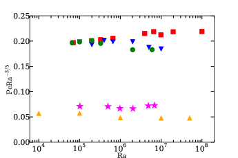
Figure 5: (Color online) Plot of normalized Péclet number ($\mathrm{Pe}\mathrm{Ra}^{-3/5}$) vs. Ra for the free-slip runs with $\mathrm{Pr}=\infty$ (red squares), $\mathrm{Pr}=10^{2}$ (blue down-pointing triangles), and $\mathrm{Pr}=10^{3}$ (green circles); and for the no-slip runs with $\mathrm{Pr}=10^{2}$ (orange triangles) and $\mathrm{Pr}=10^{3}$ (pink stars; data from Silano, et al. Silano et al. (2010)). The prefactors for the no-slip runs are lower than those for the free-slip runs.

Since the Reynolds number $\mathrm{Re}=\mathrm{Pe}/\mathrm{Pr}$, $\mathrm{Re}=0$ for $\mathrm{Pr}=\infty$, and $\mathrm{Re}$ is small for $\mathrm{Pr}\gg 1$. Hence the flow is viscous when the Prandtl number is large or infinite. Note however that the Reynolds number tends to become larger than one (yet near one) for very large Ra (see Table 1).

IV.3 Nusselt number scaling

Nusselt number is defined as the ratio of total heat flux to the conductive heat flux, i.e.,

$$\mathrm{Nu}=\frac{\kappa\Delta/d+\langle u_{z}T\rangle}{\kappa\Delta/d}=1+\langle\frac{u_{z}d}{\kappa}\frac{\theta_{\mathrm{res}}}{\Delta}\rangle=1+\langle u^{\prime}_{z}\theta^{\prime}_{\mathrm{res}}\rangle,$$ (30)

where $\theta^{\prime}_{\mathrm{res}}=\theta_{\mathrm{res}}/\Delta$ is the normalized temperature fluctuation without $\hat{\theta}(0,0,2n)$ modes, and $u^{\prime}_{z}=u_{z}d/\kappa$. The absence of $(0,0,2n)$ Fourier modes in the above expression is due to the fact that $\hat{u}_{z}(0,0,2n)=0$ (see § II).

The above expression for Nu can be rewritten as Verma et al. (2012); Verma et al. (2013a)

$$\mathrm{Nu}-1=\langle u_{z}^{\prime}\theta^{\prime}_{\mathrm{res}}\rangle=C_{u\theta}(\mathrm{Ra})\langle u_{z}^{\prime 2}\rangle^{1/2}_{V}\langle\theta^{\prime 2}_{\mathrm{res}}\rangle_{V}^{1/2},$$ (31)

where the correlation function between the vertical velocity and temperature fields $C_{u\theta}(\mathrm{Ra})$ is

$$C_{u\theta}(\mathrm{Ra})=\left\langle\frac{\langle u_{z}^{\prime}\theta^{\prime}_{\mathrm{res}}\rangle_{V}}{\langle u_{z}^{\prime 2}\rangle_{V}^{1/2}\langle\theta^{\prime 2}_{\mathrm{res}}\rangle_{V}^{1/2}}\right\rangle_{t}.$$ (32)

Here, $V$ and $t$ stand for the volume and temporal averages respectively. Our numerical data reveal that $C_{u\theta}(\mathrm{Ra})=a_{4}\mathrm{Ra}^{-0.15}$, as exhibited in Fig. 6. We observe that $C_{u\theta}=(3.8\pm 0.6)\mathrm{Ra}^{-0.15\pm 0.01}$ for $\mathrm{Pr}=\infty$, $C_{u\theta}=(2.9\pm 0.6)\mathrm{Ra}^{-0.13\pm 0.02}$ for $\mathrm{Pr}=10^{2}$, and $C_{u\theta}=(3.4\pm 0.2)\mathrm{Ra}^{-0.14\pm 0.01}$ for $\mathrm{Pr}=10^{3}$.

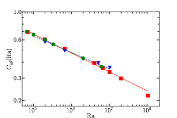
Figure 6: (Color online) Plots of correlation function between the vertical velocity and temperature fields $C_{u\theta}(\mathrm{Ra})$ vs. Ra for the free-slip runs with $\mathrm{Pr}=\infty$ (red squares), $\mathrm{Pr}=10^{2}$ (blue down-pointing triangles), and $\mathrm{Pr}=10^{3}$ (green circles). $C_{u\theta}\approx a_{4}\mathrm{Ra}^{-0.15}$.

Eq. (31) can be expressed as

$$\mathrm{Nu}-1\approx\mathrm{Nu}\approx C_{u\theta}(\mathrm{Ra})\langle u_{z}^{\prime 2}\rangle^{1/2}_{V}\langle\theta^{\prime 2}_{\mathrm{res}}\rangle_{V}^{1/2}.$$ (33)

Using the scaling relations $C_{u\theta}=a_{4}\mathrm{Ra}^{-0.15}$, $\mathrm{Pe}=a_{3}\mathrm{Ra}^{1-\zeta}$, and $\theta_{\mathrm{res}}=a_{1}\mathrm{Ra}^{-\delta}$, we deduce that

$$\mathrm{Nu}=a_{1}a_{3}a_{4}\mathrm{Ra}^{1-\zeta-\delta-0.15}=a_{5}\mathrm{Ra}^{0.32},$$ (34)

with $\zeta\approx 0.38$ and $\delta\approx 0.15$, and $a_{5}=a_{1}a_{3}a_{4}$. Our arguments show that a subtle variations of Pe and $\theta^{\prime}$ with respect to $\mathrm{Ra}$, and the correlation between the vertical velocity and temperature fields yield $\mathrm{Nu}\approx a_{5}\mathrm{Ra}^{0.32}$.

Figure 7: (Color online) Normalized Nusselt number ($\mathrm{Nu}\mathrm{Ra}^{-0.29}$) as a function of Ra for free-slip runs with $\mathrm{Pr}=\infty$ (red squares), $\mathrm{Pr}=10^{2}$ (blue down-pointing triangles), $\mathrm{Pr}=10^{3}$ (green circles), and for Pr = $\infty$ (2D) (open red squares, data taken from Hansen, et al. Hansen et al. (1990)); and for no-slip runs with $\mathrm{Pr}=10^{2}$ (2D) (orange triangles), $\mathrm{Pr}=10^{2}$ (pink stars, data taken from Silano, et al. Silano et al. (2010)), and $\mathrm{Pr}=10^{3}$ (black hexagons, data taken from Silano, et al. Silano et al. (2010)). Experimental data of Xia, et al. Xia et al. (2002) for $\mathrm{Pr}=205$ and $\mathrm{Pr}=818$ are shown as cyan filled pentagons and burlywood diamonds respectively.

Scaling relations for $\mathrm{Pr}=\infty$, $10^{2}$, and $10^{3}$ (free-slip runs) computed using our numerical data are $\mathrm{Nu}=(0.23\pm 0.02)\mathrm{Ra}^{0.32\pm 0.01}$, $\mathrm{Nu}=(0.32\pm 0.07)\mathrm{Ra}^{0.30\pm 0.01}$, and $\mathrm{Nu}=(0.29\pm 0.01)\mathrm{Ra}^{0.31\pm 0.01}$ respectively. In addition, for the no-slip run, $\mathrm{Nu}=(0.14\pm 0.03)\mathrm{Ra}^{0.29\pm 0.01}$ for $\mathrm{Pr}=10^{2}$. The prefactor for the free-slip runs is higher than that for the no-slip runs (data from Silano, et al. Silano et al. (2010) and Xia, et al. Xia et al. (2002)), which is reasonable since the heat transport is enhanced for the free-slip runs due to lower friction at the top and bottom plates (see Fig. 7). Also, for $\mathrm{Pr}=\infty$ with free-slip run, we observe that $a_{1}\approx 0.58$, $a_{3}\approx 0.20$, and $a_{4}\approx 3.8$, and consequently $a_{5}\approx 0.44$, which is in a reasonable agreement with the observed $a_{5}\approx 0.23$. Similar consistency is observed for $\mathrm{Pr}=10^{2}$ and $10^{3}$ as well. Thus, our scaling results for $\theta$, Pe and Nu are consistent with each other.

The aforementioned scaling results are in good agreement with GL scaling Grossmann and Lohse (2001), according to which $\mathrm{Nu}=0.17\mathrm{Ra}^{1/3}$ in I${}_{\infty}^{<}$ regime. Our results are also consistent with the experimental results of Xia, et al. Xia et al. (2002) for Pr = 205 and 818, and the numerical results of Silano, et al. Silano et al. (2010) and Roberts Roberts (1979) for large Pr simulations (see Fig. 7).

IV.4 Scaling of dissipation rates

In Section II, we derived relationships between the normalized dissipation rates and the Nusselt number. In this subsection we compute the normalized dissipation rates $C_{\epsilon_{u}}$, $C_{\epsilon_{T},1},C_{\epsilon_{T},2}$ using numerical data and compare them with the exact results.

From the exact relationship between the viscous dissipation rate and the Nusselt number (Eq. (23)), we obtain

$$C_{\epsilon_{u}}=\frac{(\mathrm{Nu}-1)\mathrm{Ra}}{\mathrm{Pe}^{2}}\approx\frac{a_{5}}{a_{3}^{2}}\mathrm{Ra}^{\gamma+2\zeta-1}=\frac{a_{5}}{a_{3}^{2}}\mathrm{Ra}^{0.08}$$ (35)

using $\gamma=0.32$ and $\zeta=0.38$. For $\mathrm{Pr}=\infty$, $a_{5}\approx 0.23$ and $a_{3}\approx 0.20$ provide the prefactor to be 5.8. Fig. 8 shows the variation of $C_{\epsilon_{u}}$ with Ra for Pr = $10^{2},10^{3}$, and $\infty$. From our numerical data (Table 1) we find that $C_{\epsilon_{u}}=(3.8\pm 1.2)\mathrm{Ra}^{0.15\pm 0.02}$ for $\mathrm{Pr}=10^{2}$, $C_{\epsilon_{u}}=(3.3\pm 1.1)\mathrm{Ra}^{0.17\pm 0.02}$ for $\mathrm{Pr}=10^{3}$, and $C_{\epsilon_{u}}=(6.6\pm 1.3)\mathrm{Ra}^{0.10\pm 0.01}$ for $\mathrm{Pr}=\infty$. These computed results are in good agreement with the aforementioned estimates using exact relationships, thus they validate our computations as well as show consistency with the other scaling relations.

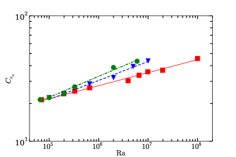
Figure 8: (Color online) Plot of normalized viscous dissipation rate $C_{\epsilon_{u}}$ vs. Ra for the free-slip runs with $\mathrm{Pr}=\infty$ (red squares), $\mathrm{Pr}=10^{2}$ (blue down-pointing triangles), and $\mathrm{Pr}=10^{3}$ (green circles). $C_{\epsilon_{u}}(\mathrm{Ra})\sim\mathrm{Ra}^{0.15}$, $\mathrm{Ra}^{0.17}$, and $\mathrm{Ra}^{0.10}$ for $\mathrm{Pr}=10^{2}$, $10^{3}$, and $\infty$ respectively.

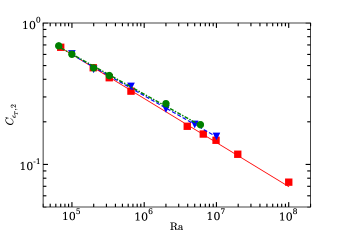
Figure 9: (Color online) Plot of normalized thermal dissipation rate $C_{\epsilon_{T},2}$ vs. Ra for the free-slip runs with $\mathrm{Pr}=\infty$ (red squares), $\mathrm{Pr}=10^{2}$ (blue down-pointing triangles), and $\mathrm{Pr}=10^{3}$ (green circles). $C_{\epsilon_{T},2}\sim\mathrm{Ra}^{-0.29}$, $\mathrm{Ra}^{-0.28}$, and $\mathrm{Ra}^{-0.31}$ for $\mathrm{Pr}=10^{2}$, $10^{3}$, and $\infty$ respectively.

According to Eq. (24), the normalized thermal dissipation rate is defined as

$$C_{\epsilon_{T},1}=\frac{\epsilon_{T}}{\kappa\Delta^{2}/d^{2}}=\mathrm{Nu}=a_{5}\mathrm{Ra}^{\gamma}.$$ (36)

Thus $C_{\epsilon_{T},1}$ has a same scaling as the Nusselt number (see Table 1). The scaling of the other normalized thermal dissipation rate is more complex. Eq. (25) yields

$$C_{\epsilon_{T},2}=\frac{\epsilon_{T}}{U_{L}\theta_{L}^{2}/d}=\frac{\mathrm{Nu}}{\mathrm{Pe}}\left(\frac{\Delta}{\theta_{L}}\right)^{2}.$$ (37)

Using the scaling of Nu, Pe and $\theta_{L}$, we deduce

$$C_{\epsilon_{T},2}=\frac{a_{5}}{a_{3}a_{2}^{2}}\mathrm{Ra}^{\gamma+\zeta-1}=\frac{a_{5}}{a_{3}a_{2}^{2}}\mathrm{Ra}^{-0.30},$$ (38)

with $\gamma=0.32$ and $\zeta=0.38$. Using the constants $a_{i}$’s, the prefactor is approximately 14 for $\mathrm{Pr}=\infty$. Similar exponents and prefactors are observed for other large Pr simulations. In Fig. 9 we plot $C_{\epsilon_{T},2}$ vs. Ra, which exhibits $C_{\epsilon_{T},2}=(17\pm 5.1)\mathrm{Ra}^{-0.29\pm 0.02}$ for $\mathrm{Pr}=10^{2}$, $C_{\epsilon_{T},2}=(16\pm 4.1)\mathrm{Ra}^{-0.28\pm 0.02}$ for $\mathrm{Pr}=10^{3}$, and $C_{\epsilon_{T},2}=(22\pm 2.2)\mathrm{Ra}^{-0.31\pm 0.01}$ for $\mathrm{Pr}=\infty$. These numerical results are in good agreement with the theoretical estimates computed earlier. For Pr = 0.7, Emran and Schumacher Emran and Schumacher (2008, 2012) also observed nearly similar scaling for thermal dissipation rate. They estimated thermal dissipation rates separately in the bulk and boundary layers, as well as in the plume-dominated regions and in the turbulent background.

The aforementioned scaling of the dissipation rates and their consistency with other global quantities like Nu and Pe indicate consistency of our arguments. These results are summarized in Table 4 for a free-slip simulation with $\mathrm{Pr}=\infty$, and in Table 5 for a no-slip simulation with $\mathrm{Pr}=10^{2}$. The exponents and the prefactors are nearly the same for all $\mathrm{Pr}\geq 10^{2}$.

After our discussion on the global quantities, we turn to the computations of energy and entropy spectra, as well as their fluxes.

V Energy and entropy spectra

Energy and entropy contained in a wavenumber shell of radius $k$ are called the energy spectrum $E_{u}(k)$ and entropy spectrum $E_{\theta}(k)$ respectively, i.e.,

$$E_{u}(k) = \sum_{k\leq|{\bf k^{\prime}}|<k+1}\frac{|\hat{\mathbf{u}}(\mathbf{k}^{\prime})|^{2}}{2},$$ (39)

$$E_{\theta}(k) = \sum_{k\leq|{\bf k^{\prime}}|<k+1}\frac{|\hat{\theta}(\mathbf{k^{\prime}})|^{2}}{2}.$$ (40)

Nonlinear interactions lead to a transfer of energy and entropy from smaller wavenumber modes to larger wavenumber modes. These transfers are quantified using energy flux $\Pi_{u}(k_{0})$ and entropy flux $\Pi_{\theta}(k_{0})$, which are the fluxes coming out of a wavenumber sphere of radius $k_{0}$ Verma (2004); Mishra and Verma (2010)

$$\Pi_{u}(k_{0})=\sum_{k\geq k_{0}}\sum_{p<k_{0}}\delta_{\mathbf{k},\mathbf{p}+\mathbf{q}}\Im([\mathbf{k}\cdot\hat{\mathbf{u}}(\mathbf{q})][\hat{\mathbf{u}}^{*}(\mathbf{k})\cdot\hat{\mathbf{u}}(\mathbf{p})]),$$ (41)

$$\Pi_{\theta}(k_{0})=\sum_{k\geq k_{0}}\sum_{p<k_{0}}\delta_{\mathbf{k},\mathbf{p}+\mathbf{q}}\Im([\mathbf{k}\cdot\hat{\mathbf{u}}(\mathbf{q})][\hat{\theta}^{*}(\mathbf{k})\cdot\hat{\theta}(\mathbf{p})]),$$ (42)

where $\Im$ is the imaginary part of the argument, and ${\mathbf{k},\mathbf{p},\mathbf{q}}$ are the wavenumbers of a triad with ${\mathbf{k}=\mathbf{p}+\mathbf{q}}$.

For $\mathrm{Pr}=\infty$, the momentum equation (Eq. (8)) yields

$$\alpha g(\theta_{\mathrm{res}})_{l}\approx\frac{\nu u_{l}}{l^{2}}.$$ (43)

We take $(\theta_{\mathrm{res}})_{l}=\mathrm{Ra}^{-\delta}\theta_{l}$ with $\delta$ defined in Eq. (26). We also assume a constant entropy flux, which yields

$$\epsilon_{\theta}=\frac{\theta_{L}^{2}U_{L}}{d}C_{\epsilon_{\theta},2}=\frac{\theta_{l}^{2}u_{l}}{l}C_{\epsilon_{\theta},2}.$$ (44)

We use the expressions of $\theta_{L}$ and $U_{L}$ derived earlier (Eqs. (27) and (29)). After substitutions of these expressions in the above equations we obtain

$$u_{l} = (a_{2}^{2}a_{3})^{\frac{1}{3}}\frac{\kappa}{d}\mathrm{Ra}^{\frac{1}{3}(3-2\delta-\zeta)}\left(\frac{l}{d}\right)^{\frac{5}{3}},$$ (45)

$$\theta_{l} = (a_{2}^{2}a_{3})^{\frac{1}{3}}\Delta\mathrm{Ra}^{\frac{1}{3}(\delta-\zeta)}\left(\frac{l}{d}\right)^{-\frac{1}{3}},$$ (46)

and therefore the energy and entropy spectra are

$$E_{u}(k) = (a_{2}^{2}a_{3})^{\frac{2}{3}}d\left(\frac{\kappa}{d}\right)^{2}\mathrm{Ra}^{\frac{2}{3}(3-2\delta-\zeta)}(kd)^{-\frac{13}{3}},$$ (47)

$$E_{\theta}(k) = (a_{2}^{2}a_{3})^{\frac{2}{3}}d\Delta^{2}\mathrm{Ra}^{\frac{2}{3}(\delta-\zeta)}(kd)^{-\frac{1}{3}}.$$ (48)

We define normalized spectra $\tilde{E}_{u}(k)$ and $\tilde{E}_{\theta}(k)$ as

$$\tilde{E}_{u}(k) = \frac{E_{u}(k)}{d\left(\frac{\kappa}{d}\right)^{2}\mathrm{Ra}^{\frac{2}{3}(3-2\delta-\zeta)}}=(a_{2}^{2}a_{3})^{\frac{2}{3}}(kd)^{-\frac{13}{3}},$$ (49)

$$\tilde{E}_{\theta}(k) = \frac{E_{\theta}(k)}{d\Delta^{2}\mathrm{Ra}^{\frac{2}{3}(\delta-\zeta)}}=(a_{2}^{2}a_{3})^{\frac{2}{3}}(kd)^{-\frac{1}{3}}.$$ (50)

For $\mathrm{Pr}=\infty$, the prefactor $(a_{2}^{2}a_{3})^{2/3}$ computed using $a_{i}$’s discussed earlier is approximately $6.3\times 10^{-2}$.

In Fig. 10 we plot kinetic spectrum $\tilde{E}_{u}(k)$ and normalized kinetic spectrum $\tilde{E}_{u}(k)k^{13/3}$ for $(\mathrm{Pr}=\infty,\mathrm{Ra}=10^{8})$ and $(\mathrm{Pr}=10^{2},\mathrm{Ra}=10^{7})$. Normalized kinetic spectrum appears nearly constant for more than one decade of wavenumber with $\tilde{E}_{u}(k)\approx(0.06\pm 0.02)k^{-13/3}$. This result is in a very good agreement with the predictions based on scaling arguments. Note that the $E_{u}(k)$ follows neither the Bolgiano-Obukhov nor the Kolmogorov-Obukhov scaling L’vov and Falkovich (1992); Mishra and Verma (2010) since the velocity field is viscous. The above scaling law for the kinetic energy spectrum also holds for $\mathrm{Pr}=10^{3}$ for free-slip boundary condition, and for $\mathrm{Pr}=10^{2}$ for no-slip boundary condition, as exhibited in Fig. 11. For better statistics, we average approximately 35 frames for free-slip data; the no-slip data however is not averaged. The prefactors for the free-slip runs are larger than those for the no-slip run due to lower frictional forces for the free-slip convection. We however remark that the data points for the no-slip boundary condition are not uniformly distributed, which necessitates interpolation of the data points to a uniform mesh. It is possible that the sawtooth-like spectrum at high wavenumbers could be due to the interpolation process. Also, the sharp viscous boundary layer for the no-slip box could produce fluctuations in the spectrum.

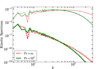
Figure 10: (Color online) Kinetic energy spectrum $\tilde{E}_{u}(k)$ for $\mathrm{Pr}=\infty,\mathrm{Ra}=10^{8}$ (thick red dashed curve), and for $\mathrm{Pr}=10^{2},\mathrm{Ra}=10^{7}$ (thick green curve). The respective normalized kinetic spectra $\tilde{E}_{u}(k)k^{13/3}$ (thin curves) are approximate constants in the powerlaw range, thus $E_{u}(k)\sim k^{-13/3}$.

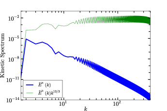
Figure 11: (Color online) For no-slip box with $\mathrm{Pr}=10^{2}$, and $\mathrm{Ra}=10^{7}$: the kinetic energy spectrum $\tilde{E}_{u}(k)$ (thick blue curve), and the compensated kinetic energy spectrum $\tilde{E}_{u}(k)k^{13/3}$ (thin green curve). The scaling is similar to that for the free-slip runs, except for a smaller prefactor.

The entropy spectrum, however, is more complex. The entropy spectrum $\tilde{E}_{\theta}(k)$ exhibited in Fig. 12 for $(\mathrm{Pr}=\infty,\mathrm{Ra}=10^{8})$ and $(\mathrm{Pr}=10^{2},\mathrm{Ra}=10^{7})$ exhibits dual branches. The upper branch, which corresponds to the $\hat{\theta}(0,0,2n)$ Fourier modes, follows $k^{-2}$ energy spectrum since $\hat{\theta}(0,0,2n)\approx-1/(2n\pi)$ (see § II and Mishra and Verma (2010)). The lower branch is the energy spectrum of the Fourier modes other than $\hat{\theta}(0,0,2n)$, and it follows nearly a flat spectrum. The nature of the entropy spectrum is very different from our phenomenological predictions that $E_{\theta}(k)\propto k^{-1/3}$. This discrepancy is due to the boundary condition (the conducting plates) which yields significant $\hat{\theta}(0,0,2n)$ branch (see § II and Mishra and Verma Mishra and Verma (2010)). Similar behavior is observed for $\mathrm{Pr}=10^{3}$ with the free-slip boundary condition, and for $\mathrm{Pr}=10^{2}$ with no-slip boundary condition, as exhibited in Fig. 13.

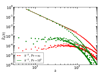
Figure 12: (Color online) Plot of entropy spectrum $\tilde{E}_{\theta}(k)$ vs. $k$ for $\mathrm{Pr}=\infty,\mathrm{Ra}=10^{8}$ (red filled circles) and for $\mathrm{Pr}=10^{2},\mathrm{Ra}=10^{7}$ (green filled squares). The upper branches of the spectra represent $\hat{\theta}(0,0,2n)$ modes that exhibit $k^{-2}$ scaling (red dashed and green solid curves). The lower branch is somewhat flat.

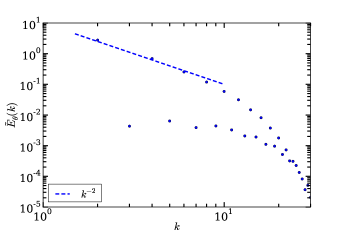
Figure 13: (Color online) Plot of entropy spectrum $\tilde{E}_{\theta}(k)$ for $\mathrm{Pr}=10^{2},\mathrm{Ra}=10^{7}$ with no-slip boundary condition. The spectrum exhibits similar scaling as large-Pr free-slip runs.

We also compute the entropy flux $\Pi_{\theta}(k_{0})$ using the numerical data. In Fig. 14 we plot $\Pi_{\theta}(k)$ for $\mathrm{Pr}=\infty$ and $\mathrm{Ra}=10^{8}$, and for $\mathrm{Pr}=10^{2}$ and $\mathrm{Ra}=10^{7}$. The plots indicate a nearly constant entropy flux in the powerlaw regime. The constancy of $\Pi_{\theta}(k)$ is due to the dominance of nonlinear term in the temperature equation. The kinetic energy flux $\Pi_{u}(k)$ however is zero for $\mathrm{Pr}=\infty$ due to the absence of the nonlinearity in the velocity equation. For large Pr runs, $\Pi_{u}(k)$ is very small due to weak nonlinearity.

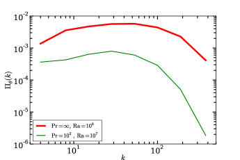
Figure 14: (Color online) Plot of entropy flux $\Pi_{\theta}(k)$ vs. $k$ for $\mathrm{Pr}=\infty,\mathrm{Ra}=10^{8}$ (thick red curve), and for $\mathrm{Pr}=10^{2},\mathrm{Ra}=10^{7}$ (thin green curve). The fluxes are approximate constants in the powerlaw range.

In Table 4 we summarize the scaling results for $\mathrm{Pr}=\infty$ simulation under free-slip boundary condition, and Table 5 for $\mathrm{Pr}=10^{2}$ simulation under no-slip boundary condition. Here we list the theoretically-estimated and numerically-computed values. The two sets of values are in good agreement with each other. The scaling for large Pr ($\mathrm{Pr}\geq 10^{2}$) RBC is very similar to that for $\mathrm{Pr}=\infty$ RBC. Our data for no-slip boundary condition are somewhat limited at present.

Table 4: Summary of the scaling functions for various quantities for free-slip runs with $\mathrm{Pr}=\infty$. The estimated values using analytical arguments agree quite well with the numerically computed ones. The formulas for the scaling functions using $a_{i}$’s are listed in the second column.

Quantity	Formula	Estimated	Computed
$\theta_{\mathrm{res}}/\Delta$	$a_{1}\mathrm{Ra}^{-\delta}$	$-$	$(0.59\pm 0.08)\mathrm{Ra}^{-0.15\pm 0.01}$
$\theta_{\mathrm{rms}}/\Delta$	$a_{2}$	$-$	$(0.29\pm 0.01)$
Pe	$a_{3}\mathrm{Ra}^{1-\zeta}$	$0.16\mathrm{Ra}^{0.62}$	$(0.20\pm 0.02)\mathrm{Ra}^{0.61\pm 0.01}$
$C_{u\theta}$	$a_{4}\mathrm{Ra}^{-0.15}$	$-$	$(3.8\pm 0.6)\mathrm{Ra}^{-0.15\pm 0.01}$
Nu	$a_{5}\mathrm{Ra}^{\gamma}$	$0.43\mathrm{Ra}^{0.32}$	$(0.23\pm 0.02)\mathrm{Ra}^{0.32\pm 0.01}$
$C_{\epsilon_{u}}$	$(a_{5}/a_{3}^{2})\mathrm{Ra}^{\gamma+2\zeta-1}$	$5.8\mathrm{Ra}^{0.08}$	$(6.6\pm 1.3)\mathrm{Ra}^{0.10\pm 0.01}$
$C_{\epsilon_{T},2}$	$a_{5}/(a_{3}a_{2}^{2})\mathrm{Ra}^{\gamma+\zeta-1}$	$14\mathrm{Ra}^{-0.30}$	$(22\pm 2.2)\mathrm{Ra}^{-0.31\pm 0.01}$
$\tilde{E}_{u}(k)$	$(a_{2}^{2}a_{3})^{2/3}k^{-13/3}$	$0.063k^{-13/3}$	$(0.06\pm 0.02)k^{-13/3}$
$\tilde{E}_{\theta}(k)$	$(a_{2}^{2}a_{3})^{2/3}k^{-1/3}$	$0.063k^{-1/3}$	Dual branches

Table 5: Summary of the scaling functions for various quantities for no-slip runs with $\mathrm{Pr}=10^{2}$. The computed $\theta_{\mathrm{rms}}$ is taken from Silano, et al. Silano et al. (2010). The estimated Pe and Nu scaling are taken from Grossmann and Lohse’s Grossmann and Lohse (2001) theoretical work (the I${}^{<}_{\infty}$ regime).

Quantity	Estimated	Computed
$\theta_{\mathrm{rms}}$	$-$	$(0.12\pm 0.02)\Delta$
Pe	$0.038\mathrm{Ra}^{2/3}$	$(0.05\pm 0.01)\mathrm{Ra}^{0.60\pm 0.01}$
Nu	$0.17\mathrm{Ra}^{1/3}$	$(0.14\pm 0.03)\mathrm{Ra}^{0.29\pm 0.01}$
$\tilde{E}_{u}(k)$	$0.008k^{-13/3}$	$(0.006\pm 0.004)k^{-13/3}$
$\tilde{E}_{\theta}(k)$	$0.008k^{-1/3}$	Dual branches

VI Conclusions and discussions

In this paper we derive scaling properties of the large-scale quantities (e.g., Péclet and Nusselt numbers), as well as that of energy and entropy spectra for very large and infinite Prandtl number convection. The equation for the velocity field is linear for $\mathrm{Pr}=\infty$ limit that helps us derive relationships between various quantities. These scaling relations are verified using numerical simulations for infinite and large Prandtl numbers ($\mathrm{Pr}\geq 10^{2}$). We observe that the scaling of flows with large Prandtl number ($\mathrm{Pr}\geq 10^{2}$) is same as that for the infinite Prandtl number, thus making them $\mathrm{Pr}$-independent. Our results are consistent with the earlier theoretical predictions of Grossmann and Lohse Grossmann and Lohse (2001), experimental results of Xia, et al. Xia et al. (2002), and the numerical results of Silano, et al. Silano et al. (2010). Note however that the analytical work of Grossmann and Lohse Grossmann and Lohse (2001) is based on Shraiman and Siggia’s Shraiman and Siggia (1990) exact relations and modelling of the dissipation rates at the bulk and boundary layers. While our theoretical work is based on the dimensional and scaling analysis of the dynamical equation of the velocity and temperature fields, as well as several inputs from the numerical simulations.

A summary of our results is as follows.

1. The temperature field is dominated by the Fourier modes $\hat{\theta}(0,0,2n)$, which are approximately $-1/(2n\pi)$ for small $n$ in accordance with the predictions by Mishra and Verma Mishra and Verma (2010). The modes other than $\hat{\theta}(0,0,2n)$ are termed as “residual modes” whose rms fluctuations scale as $\mathrm{Ra}^{-\delta}$ with $\delta\approx 0.15$. Due to the dominance of $\hat{\theta}(0,0,2n)$ modes, the large-scale temperature fluctuations follow $\theta_{\mathrm{rms}}\sim\Delta$ for the free-slip boundary condition, where $\Delta$ is the temperature difference between the hot and cold plates. However the numerical results of Silano, et al. Silano et al. (2010) for the no-slip boundary condition exhibit the above behaviour (with a smaller prefactor) for lower $\mathrm{Ra}$, but $\theta_{\mathrm{rms}}$ appear to decrease slowly with $\mathrm{Ra}$ for larger $\mathrm{Ra}$. We show that the residual modes play a very important role in the scaling of Nusselt number, energy spectrum, etc.

2. The Péclet number, which is proportional to the large-scale velocity, scales as $\mathrm{Ra}^{1-\zeta}$ with $\zeta\approx 0.38$. Note that the Reynolds number in the large Pr limit is small, i.e., $\mathrm{Re}\lessapprox 1$. These results are consistent with the theoretical predictions of GL Grossmann and Lohse (2001) and the numerical results of Silano, et al. Silano et al. (2010).

3. The Nusselt number scales as $\mathrm{Ra}^{\gamma}$ with the exponent lying in the range from 0.30 to 0.32, which is consistent with the results of Grossmann and Lohse Grossmann and Lohse (2001), Silano, et al. Silano et al. (2010), Roberts Roberts (1979), Xia, et al. Xia et al. (2002), and Constantin and Doering Constantin and Doering (1999). This scaling arises due to a complex interplay between the residual modes, Péclet number, and the velocity-temperature correlation.

4. The normalized viscous and thermal dissipation rates are functions of Ra. We observe that

   $$C_{\epsilon_{u}} = \frac{\epsilon_{u}}{\nu U_{L}^{2}/d^{2}}\approx\mathrm{Ra}^{b_{1}},$$ (51)

   $$C_{\epsilon_{T},2} = \frac{\epsilon_{T}}{U_{L}\theta_{L}^{2}/d}\approx\mathrm{Ra}^{-b_{2}},$$ (52)

   with $b_{1}\approx 0.10$ and $b_{2}\approx 0.31$. These relations are consistent with the Nu scaling derived using the exact relations of Shraiman and Siggia Shraiman and Siggia (1990). Here we derive an explicit Ra-dependent normalized dissipation rates for large Pr for the first time.

5. Using analytical arguments, we derive that the energy spectrum $E_{u}(k)\sim k^{-13/3}$. Our simulations verify this power law in the powerlaw range for both the free-slip and no-slip boundary conditions.

6. We predict that the entropy spectrum $E_{\theta}(k)\sim k^{-1/3}$. Unfortunately this power law is not observed in the numerical simulations. Instead, we find dual entropy spectra consisting of an upper branch with $k^{-2}$ spectrum corresponding to $\hat{\theta}(0,0,2n)\approx-1/(2n\pi)$, and a nearly flat lower branch. The dual branching is due to the presence of boundary layers Mishra and Verma (2010).

7. Our numerical simulations show that the free-slip and no-slip boundary conditions provide similar scaling relations for the global quantities, as well as for the energy and entropy spectra. However, the prefactors of the Péclet and Nusselt numbers, and that of energy spectrum are smaller for the no-slip condition than those for the free-slip boundary condition. This discrepancy is due to a smaller frictional force experienced by the flow for the free-slip boundary condition. The similarities of the scaling functions between the free-slip and no-slip convection are due to the dominance of the large-scale flows, which have similar structures for both the free-slip and no-slip boundary conditions. Note that viscous boundary layers pervade the whole box for $\mathrm{Pr}=\infty$, hence they determine the properties of the bulk flow.

In summary, we derived scaling relations for large-scale quantities, and energy and entropy spectra for large and infinite Prandtl number convection. The scaling properties are independent of the Prandtl number in this regime. Our analytical and numerical results are consistent with earlier results of Grossmann and Lohse Grossmann and Lohse (2001), Silano, et al. Silano et al. (2010), and Xia, et al. Xia et al. (2002).

References

- Ahlers et al. (2009a) G. Ahlers, S. Grossmann, and D. Lohse, Rev. Mod. Phys. 81, 503 (2009a).
- Lohse and Xia (2010) D. Lohse and K. Q. Xia, Ann. Rev. Fluid Mech. 42, 335 (2010).
- Kraichnan (1962) R. Kraichnan, Phys. Fluids 5, 1374 (1962).
- Grossmann and Lohse (2000) S. Grossmann and D. Lohse, J. Fluid Mech. 407, 27 (2000).
- Grossmann and Lohse (2001) S. Grossmann and D. Lohse, Phys. Rev. Lett. 86, 3316 (2001).
- Grossmann and Lohse (2002) S. Grossmann and D. Lohse, Phys. Rev. E 66, 016305 (2002).
- Grossmann and Lohse (2004) S. Grossmann and D. Lohse, Phys. Fluids 16, 4462 (2004).
- Grossmann and Lohse (2011) S. Grossmann and D. Lohse, Phys. Fluids 23, 045108 (2011).
- Stevens et al. (2013) R. Stevens, E. P. Poel, S. Grossmann, and D. Lohse, J. Fluid Mech. 730, 295 (2013).
- Shraiman and Siggia (1990) B. I. Shraiman and E. D. Siggia, Phys. Rev. A 42, 3650 (1990).
- Whitehead and Doering (2011) J. P. Whitehead and C. R. Doering, Phys. Rev. Lett. 106, 244501 (2011).
- Ierley et al. (2006) G. R. Ierley, R. R. Kerswell, and S. C. Plasting, J. Fluid Mech. 560, 159 (2006).
- Constantin and Doering (1999) P. Constantin and C. R. Doering, J. Stat. Phys. 94, 159 (1999).
- Castaing et al. (1989) B. Castaing, G. Gunaratne, L. Kadanoff, A. Libchaber, and F. Heslot, J. Fluid Mech. 204, 1 (1989).
- Cioni et al. (1997) S. Cioni, S. Ciliberto, and J. Sommeria, J. Fluid Mech. 335, 111 (1997).
- Glazier et al. (1999) J. Glazier, T. Segawa, A. Naert, and M. Sano, Nature 398, 307 (1999).
- Niemela et al. (2000) J. J. Niemela, L. Skrbek, K. R. Sreenivasan, and R. J. Donnelly, Nature 404, 837 (2000).
- Ahlers and Xu (2001) G. Ahlers and X. Xu, Phys. Rev. Lett. 86, 3320 (2001).
- Niemela and Sreenivasan (2003) J. J. Niemela and K. R. Sreenivasan, J. Fluid Mech. 481, 355 (2003).
- Urban et al. (2012) P. Urban, P. Hanzelka, T. Kralik, V. Musilova, A. Srnka, and L. Skrbek, Phys. Rev. Lett. 109, 154301 (2012).
- Funfschilling et al. (2009) D. Funfschilling, E. Bodenschatz, and G. Ahlers, Phys. Rev. Lett. 103, 014503 (2009).
- Ahlers et al. (2009b) G. Ahlers, D. Funfschilling, and E. Bodenschatz, New J. Phys. 11, 123001 (2009b).
- He et al. (2012) X. He, D. Funfschilling, H. Nobach, E. Bodenschatz, and G. Ahlers, Phys. Rev. Lett. 108, 024502 (2012).
- Chavanne et al. (1997) X. Chavanne, F. Chillà, B. Castaing, B. Hébral, B. Chabaud, and J. Chaussy, Phys. Rev. Lett. 79, 3648 (1997).
- Roche et al. (2001) P. E. Roche, B. Castaing, B. Chabaud, and B. Hébral, Phys. Rev. E 63, 045303(R) (2001).
- Kerr (1996) R. Kerr, J. Fluid Mech. 310, 139 (1996).
- Verzicco and Camussi (1999) R. Verzicco and R. Camussi, J. Fluid Mech. 383, 55 (1999).
- Kerr and Herring (2000) R. Kerr and J. Herring, J. Fluid Mech. 419, 325 (2000).
- Lohse and Toschi (2003) D. Lohse and F. Toschi, Phys. Rev. Lett. 90, 034502 (2003).
- Verzicco and Sreenivasan (2008) R. Verzicco and K. R. Sreenivasan, J. Fluid Mech. 595, 203 (2008).
- Stevens et al. (2010a) R. Stevens, R. Verzicco, and D. Lohse, J. Fluid Mech. 643, 495 (2010a).
- Stevens et al. (2011) R. Stevens, D. Lohse, and R. Verzicco, J. Fluid Mech. 688, 31 (2011).
- Verma et al. (2012) M. K. Verma, P. K. Mishra, A. Pandey, and S. Paul, Phys. Rev. E 85, 016310 (2012).
- Verma et al. (2013a) M. K. Verma, A. Pandey, P. K. Mishra, and M. Chandra, arXiv:1301.1240 (2013a).
- Xia et al. (2002) K.-Q. Xia, S. Lam, and S.-Q. Zhou, Phys. Rev. Lett. 88, 064501 (2002).
- Lam et al. (2002) S. Lam, X.-D. Shang, S.-Q. Zhou, and K.-Q. Xia, Phys. Rev. E 65, 066306 (2002).
- Silano et al. (2010) G. Silano, K. R. Sreenivasan, and R. Verzicco, J. Fluid Mech. 662, 409 (2010).
- Roberts (1979) G. O. Roberts, Geophys. Astrophys. Fluid Dyn. 12, 235 (1979).
- Hansen et al. (1990) U. Hansen, D. A. Yuen, and S. E. Kroening, Phys. Fluids 2, 2157 (1990).
- Schmalzl et al. (2002) J. Schmalzl, M. Breuer, and U. Hansen, Geophys. Astrophys. Fluid Dyn. 96, 381 (2002).
- Breuer et al. (2004) M. Breuer, S. Wessling, J. Schmalzl, and U. Hansen, Phys. Rev. E 69, 026302 (2004).
- L’vov (1991) V. S. L’vov, Phys. Rev. Lett. 67, 687 (1991).
- L’vov and Falkovich (1992) V. S. L’vov and G. Falkovich, Physica D 57, 85 (1992).
- Batchelor (1959) G. K. Batchelor, J. Fluid Mech. 5, 113 (1959).
- Breuer and Hansen (2009) M. Breuer and U. Hansen, Europhys. Lett. 86, 24004 (2009).
- Mishra and Verma (2010) P. K. Mishra and M. K. Verma, Phys. Rev. E 81, 056316 (2010).
- Emran and Schumacher (2008) M. S. Emran and J. Schumacher, J. Fluid Mech. 611, 13 (2008).
- Emran and Schumacher (2012) M. S. Emran and J. Schumacher, Eur. Phys. J. E 35, 12108 (2012).
- Verma et al. (2013b) M. K. Verma, A. G. Chatterjee, K. S. Reddy, R. K. Yadav, S. Paul, M. Chandra, and R. Samtanay, Pramana 81, 617 (2013b).
- Fischer (1997) P. F. Fischer, J. Comp. Phys. 133, 84 (1997).
- Stevens et al. (2010b) R. Stevens, H. Clercx, and D. Lohse, New J. Phys. 12, 075005 (2010b).
- Busse and Whitehead (1974) F. Busse and J. Whitehead, J. Fluid Mech. 66, 67 (1974).
- Grötzbach (1983) G. Grötzbach, J. Comp. Phys. 49, 241 (1983).
- Petschel et al. (2013) K. Petschel, S. Stellmach, M. Wilczek, J. Lülff, and U. Hansen, Phys. Rev. Lett. 110, 114502 (2013).
- Verma (2004) M. K. Verma, Phys. Rep. 401, 229 (2004).