The Extended Parameter Filter

The Extended Parameter Filter

Abstract

The parameters of temporal models, such as dynamic Bayesian networks, may be modelled in a Bayesian context as static or atemporal variables that influence transition probabilities at every time step. Particle filters fail for models that include such variables, while methods that use Gibbs sampling of parameter variables may incur a per-sample cost that grows linearly with the length of the observation sequence. Storvik (2002) devised a method for incremental computation of exact sufficient statistics that, for some cases, reduces the per-sample cost to a constant. In this paper, we demonstrate a connection between Storvik’s filter and a Kalman filter in parameter space and establish more general conditions under which Storvik’s filter works. Drawing on an analogy to the extended Kalman filter, we develop and analyze, both theoretically and experimentally, a Taylor approximation to the parameter posterior that allows Storvik’s method to be applied to a broader class of models. Our experiments on both synthetic examples and real applications show improvement over existing methods.

1 Introduction

Dynamic Bayesian networks are widely used to model the processes underlying sequential data such as speech signals, financial time series, genetic sequences, and medical or physiological signals. State estimation or filtering—computing the posterior distribution over the state of a partially observable Markov process from a sequence of observations—is one of the most widely studied problems in control theory, statistics and AI. Exact filtering is intractable except for certain special cases (linear–Gaussian models and discrete HMMs), but approximate filtering using the particle filter (a sequential Monte Carlo method) is feasible in many real-world applications (Arulampalam et al., 2002; Doucet and Johansen, 2011). In the machine learning context, model parameters may be represented by static parameter variables that define the transition and sensor model probabilities of the Markov process, but do not themselves change over time (Figure 1). The posterior parameter distribution (usually) converges to a delta function at the true value in the limit of infinitely many observations. Unfortunately, particle filters fail for such models: the algorithm samples parameter values for each particle at time $t{\,{=}\,}0$, but these remain fixed; over time, the particle resampling process removes all but one set of values; and these are highly unlikely to be correct. The degeneracy problem is especially severe in high-dimensional parameter spaces, whether discrete or continuous. Hence, although learning requires inference, the most successful inference algorithm for temporal models is inapplicable.

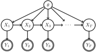
Figure 1: A state-space model with static parameters $\theta$. $X_{1:T}$ are latent states and $Y_{1:T}$ are observations.

Kantas et al. (2009) and Carvalho et al. (2010) describe several algorithms that have been proposed to solve this degeneracy problem, but the issue remains open because known algorithms either suffer from bias or computational inefficiency. For example, the “artificial dynamics” approach (Liu and West, 2001) introduces a stochastic transition model for the parameter variables, allowing exploration of the parameter space, but this may result in biased estimates. Online EM algorithms (Andrieu et al., 2005) provide only point estimates of static parameters, may converge to local optima, and are biased unless used with the full smoothing distribution. The particle MCMC algorithm (Andrieu et al., 2010) converges to the true posterior, but requires computation growing with $T$, the length of the data sequence.

The resample-move algorithm (Gilks and Berzuini, 2001) includes Gibbs sampling of parameter variables—that is, in Figure 1, $P(\theta\!\mid\!X_{1},\ldots,X_{T})$. This method requires $O(T)$ computation per sample, leading Gilks and Berzuini to propose a sampling rate proportional to $1/T$ to preserve constant-time updates. Storvik (2002) and Polson et al. (2008) observe that a fixed-dimensional sufficient statistic (if one exists) for $\theta$ can be updated in constant time. Storvik describes an algorithm for a specific family of linear-in-parameters transition models.

We show that Storvik’s algorithm is a special case of the Kalman filter in parameter space and identify a more general class of separable systems to which the same approach can be applied. By analogy with the extended Kalman filter, we propose a new algorithm, the extended parameter filter (EPF), that computes a separable approximation to the parameter posterior and allows a fixed-dimensional (approximate) sufficient statistic to be maintained. The method is quite general: for example, with a polynomial approximation scheme such as Taylor expansion any analytic posterior can be handled.

Section 2 briefly reviews particle filters and Storvik’s method and introduces our notion of separable models. Section 3 describes the EPF algorithm, and Section 4 discusses the details of a polynomial approximation scheme for arbitrary densities, which Section 4.2 then applies to estimate posterior distributions of static parameters. Section 5 provides empirical results comparing the EPF to other algorithms. All details of proofs are given in the appendix of the full version (Erol et al., 2013).

2 Background

In this section, we review state-space dynamical models and the basic framework of approximate filtering algorithms.

2.1 State-space model and filtering

Let $\Theta$ be a parameter space for a partially observable Markov process $\left\{X_{t}\right\}_{t\geq 0},\left\{Y_{t}\right\}_{t\geq 0}$ as shown in Figure 1 and defined as follows:

$$X_{0} \sim p(x_{0}\!\mid\!\theta)$$ (1)

$$X_{t}\!\mid\!x_{t-1} \sim p(x_{t}\!\mid\!x_{t-1},\theta)$$ (2)

$$Y_{t}\!\mid\!x_{t} \sim p(y_{t}\!\mid\!x_{t},\theta)$$ (3)

Here the state variables $X_{t}$ are unobserved and the observations $Y_{t}$ are assumed conditionally independent of other observations given $X_{t}$. We assume in this section that states $X_{t}$, observations $Y_{t}$, and parameters $\theta$ are real-valued vectors in $d$, $m$, and $p$ dimensions respectively. Here both the transition and sensor models are parameterized by $\theta$. For simplicity, we will assume in the following sections that only the transition model is parameterized by $\theta$; however, the results in this paper can be generalized to cover sensor model parameters.

The filtering density $p(x_{t}\!\mid\!y_{0:t},\theta)$ obeys the following recursion:

$$p(x_{t}\!\mid\!y_{0:t},\theta)=\frac{p(y_{t}\!\mid\!x_{t},\theta)p(x_{t}\!\mid\!y_{0:t-1},\theta)}{p(y_{t}\!\mid\!y_{0:t-1},\theta)}$$

$$=\frac{p(y_{t}\!\mid\!x_{t},\theta)}{p(y_{t}\!\mid\!y_{0:t-1},\theta)}\int p(x_{t-1}\!\mid\!y_{0:t-1},\theta)p(x_{t}\!\mid\!x_{t-1},\theta)dx_{t-1}$$ (4)

where the update steps for $p(x_{t}\!\mid\!y_{0:t-1},\theta)$ and $p(y_{t}\!\mid\!y_{0:t-1},\theta)$ involve the evaluation of integrals that are not in general tractable.

2.2 Particle filtering

With known parameters, particle filters can approximate the posterior distribution over the hidden state $X_{t}$ by a set of samples. The canonical example is the sequential importance sampling-resampling algorithm (SIR) (Algorithm 1).

Input: $N$: number of particles;

$y_{0},\dots,y_{T}$: observation sequence

Output: $\bar{x}_{1:T}^{1:N}$

initialize $\left\{x_{0}^{i}\right\}$ ;

for $t=1,\ldots,T$ do

       for $i=1,\dots,N$ do

             sample $x_{t}^{i}\sim p(x_{t}\!\mid\!x_{t-1}^{i})$;

             $w_{t}^{i}\leftarrow p(y_{t}\!\mid\!x_{t}^{i})$;

            

      sample $\left\{\frac{1}{N},\bar{{x}}_{t}^{i}\right\}\leftarrow$Multinomial$\left\{w_{t}^{i},{x}_{t}^{i}\right\}$;

       $\left\{{x}_{t}^{i}\right\}\leftarrow\left\{\bar{{x}}_{t}^{i}\right\}$;

      

Algorithm 1 Sequential importance sampling-resampling (SIR)

The SIR filter has various appealing properties. It is modular, efficient, and easy to implement. The filter takes constant time per update, regardless of time $T$, and as the number of particles $N\to\infty$, the empirical filtering density converges to the true marginal posterior density under suitable assumptions.

Particle filters can accommodate unknown parameters by adding parameter variables into the state vector with an “identity function” transition model. As noted in Section 1 this approach leads to degeneracy problems—especially for high-dimensional parameter spaces. To ensure that some particle has initial parameter values with bounded error, the number of particles must grow exponentially with the dimension of the parameter space.

2.3 Storvik’s algorithm

To avoid the degeneracy problem, Storvik (2002) modifies the SIR algorithm by adding a Gibbs sampling step for $\theta$ conditioned on the state trajectory in each particle (see Algorithm 2). The algorithm is developed in the SIS framework and consequently inherits the theoretical guarantees of SIS. Storvik considers unknown parameters in the state evolution model and assumes a perfectly known sensor model. His analysis can be generalized to unknown sensor models.

Storvik’s approach becomes efficient in an on-line setting when a fixed-dimensional sufficient statistic ${S}_{t}$ exists for the static parameter (i.e., when $p(\theta|{x}_{0:t})=p(\theta|{S}_{t})$ holds). The important property of this algorithm is that the parameter value simulated at time $t$ does not depend on the values simulated previously. This property prevents the impoverishment of the parameter values in particles.

Input: $N$: number of particles;

$y_{0},\dots,y_{T}$: observation sequence

Output: $\bar{x}_{1:T}^{1:N}$, $\theta^{1:N}$

initialize $\left\{x_{0}^{i}\right\}$;

for $t=1,\ldots,T$ do

       for $i=1,\dots,N$ do

             sample $\theta^{i}\sim p(\theta|{x}_{0:t-1}^{i})$;

             sample ${x}_{t}^{i}\sim p({x_{t}}|{x}_{t-1}^{i},\theta^{i})$;

             $w^{i}\leftarrow p({y}_{t}|{x}_{t}^{i})$;

            

      sample $\left\{\frac{1}{N},\bar{{x}}_{t}^{i}\right\}\leftarrow$Multinomial$\left\{w_{t}^{i},{x}_{t}^{i}\right\}$;

       $\left\{{x}_{t}^{i}\right\}\leftarrow\left\{\bar{{x}}_{t}^{i}\right\}$;

      

Algorithm 2 Storvik’s filter.

One limitation of the algorithm is that it can only be applied to models with fixed-dimensional sufficient statistics. However, Storvik (2002) analyze the sufficient statistics for a specific family.

Storvik (2002) shows how to obtain a sufficient statistic in the context of what he calls the Gaussian system process, a transition model satisfying the equation

$${x}_{t}={\mathbf{F}}_{t}^{T}\theta+\epsilon_{t},\>\>\epsilon_{t}\sim N(0,{\mathbf{Q}})$$ (5)

where $\theta$ is the vector of unknown parameters with a prior of $N(\theta_{0},{\mathbf{C}}_{0})$ and ${\mathbf{F}}_{t}={\mathbf{F}}({x}_{t-1})$ is a matrix where elements are possibly nonlinear functions of ${x}_{t-1}$. An arbitrary but known observation model is assumed. Then the standard theory states that $\theta\!\mid\!{x}_{0:t}\sim N({m}_{t},{\mathbf{C}}_{t})$ where the recursions for the mean and the covariance matrix are as follows:

$${\mathbf{D}}_{t} = {\mathbf{F}}_{t}^{T}{\mathbf{C}}_{t-1}{\mathbf{F}}_{t}+{\mathbf{Q}}$$

$${\mathbf{C}}_{t} = {\mathbf{C}}_{t-1}-{\mathbf{C}}_{t-1}{\mathbf{F}}_{t}{\mathbf{D}}_{t}^{-1}{\mathbf{F}}_{t}^{T}{\mathbf{C}}_{t-1}$$

$${m}_{t} = {m}_{t-1}+{\mathbf{C}}_{t-1}{\mathbf{F}}_{t}{\mathbf{D}}_{t}^{-1}({x}_{t}-{\mathbf{F}}_{t}^{T}{m}_{t-1})$$ (6)

Thus, ${m}_{t}$ and ${\mathbf{C}}_{t}$ constitute a fixed-dimensional sufficient statistic for $\theta$.

These updates are in fact a special case of Kalman filtering applied to the parameter space. Matching terms with the standard KF update equations (Kalman, 1960), we find that the transition matrix for the KF is the identity matrix, the transition noise covariance matrix is the zero matrix, the observation matrix for the KF is ${\mathbf{F}}_{t}$, and the observation noise covariance matrix is ${\mathbf{Q}}$. This correspondence is of course what one would expect, since the true parameter values are fixed (i.e., an identity transition). See the supplementary material (Erol et al., 2013) for the derivation.

2.4 Separability

In this section, we define a condition under which there exist efficient updates to parameters. Again, we focus on the state-space model as described in Figure 1 and Equation (3). The model in Equation (3) can also be expressed as

$$x_{t}=f_{\theta}(x_{t-1})+v_{t}$$

$$y_{t}=g(x_{t})+w_{t}$$ (7)

for some suitable $f_{\theta}$, $g$, $v_{t}$, and $w_{t}$.

Definition 1.

A system is separable if the transition function $f_{\theta}(x_{t-1})$ can be written as $f_{\theta}(x_{t-1})=l(x_{t-1})^{T}h(\theta)$ for some $l(\cdot)$ and $h(\cdot)$ and if the stochastic i.i.d. noise $v_{t}$ has log-polynomial density.

Theorem 1.

For a separable system, there exist fixed-dimensional sufficient statistics for the Gibbs density, $p(\theta\mid x_{0:T})$.

The proof is straightforward by the Fisher–Neyman factorization theorem; more details are given in the supplementary material of the full version (Erol et al., 2013).

The Gaussian system process models defined in Equation (5) are separable, since the transition function ${\mathbf{F}}_{t}^{T}\theta=({F}_{t})^{T}\theta$, but the property—and therefore Storvik’s algorithm—applies to a much broader class of systems. Moreover, as we now show, non-separable systems may in some cases be well-approximated by separable systems, constructed by polynomial density approximation steps applied to either the Gibbs distribution $p(\theta\mid x_{0:t})$ or to the transition model.

3 The extended parameter filter

Let us consider the following model.

$$x_{t}=f_{\theta}(x_{t-1})+v_{t};\>v_{t}\sim N(0,\Sigma)$$ (8)

where $x\in\mathbb{R}^{d}$,$\theta\in\mathbb{R}^{p}$ and $f_{\theta}(\cdot):\mathbb{R}^{d}\rightarrow\mathbb{R}^{d}$ is a vector-valued function parameterized by $\theta$. We assume that the transition function $f_{\theta}$ may be non-separable. Our algorithm will create a polynomial approximation to either the transition function or to the Gibbs distribution, $p(\theta\mid x_{0:t})$.

To illustrate, let us consider the transition model $f_{\theta}(x_{t-1})=\sin(\theta x_{t-1})$. It is apparent that this transition model is non-separable. If we approximate the transition function with a Taylor series in $\theta$ centered around zero

$$f_{\theta}(x_{t-1})\approx\hat{f}_{\theta}(x_{t-1})=x_{t-1}\theta-\frac{1}{3!}x_{t-1}^{3}\theta^{3}+\dots$$ (9)

and use $\hat{f}$ as an approximate transition model, the system will become separable. Then, Storvik’s filter can be applied in constant time per update. This Taylor approximation leads to a log-polynomial density of the form of Equation (12).

Our approach is analogous to that of the extended Kalman filter (EKF). EKF linearizes nonlinear transitions around the current estimates of the mean and covariance and uses Kalman filter updates for state estimation (Welch and Bishop, 1995). Our proposed algorithm, which we call the extended parameter filter (EPF), approximates a non-separable system with a separable one, using a polynomial approximation of some arbitrary order. This separable, approximate model is well-suited for Storvik’s filter and allows for constant time updates to the Gibbs density of the parameters.

Although we have described an analogy to the EKF, it is important to note that the EPF can effectively use higher-order approximations instead of just first-order linearizations as in EKF. In EKF, higher order approximations lead to intractable integrals. The prediction integral for EKF

$$p(x_{t}\mid y_{0:t-1})=\int p(x_{t-1}\mid y_{0:t-1})p(x_{t}\mid x_{t-1})dx_{t-1}$$

can be calculated for linear Gaussian transitions, in which case the mean and the covariance matrix are the tracked sufficient statistic. However, in the case of quadratic transitions (or any higher-order transitions), the above integral is no longer analytically tractable.

In the case of EPF, the transition model is the identity transition and hence the prediction step is trivial. The filtering recursion is

$$p(\theta\mid x_{0:t})\propto p(x_{t}\mid x_{t-1},\theta)p(\theta\mid x_{0:t-1}).$$ (10)

We approximate the transition $p(x_{t}\mid x_{t-1},\theta)$ with a log-polynomial density $\hat{p}$ (log-polynomial in $\theta$), so that the Gibbs density, which satisfies the recursions in equation 10, has a fixed log-polynomial structure at each time step. Due to the polynomial structure, the approximate Gibbs density can be tracked in terms of its sufficient statistic (i.e., in terms of the coefficients of the polynomial). The log-polynomial structure is derived in Section 4.2. Pseudo-code for EPF is shown in Algorithm 3.

Result: Approximate the Gibbs density $p(\theta\mid x_{0:t},y_{0:t})$ with the log-polynomial density $\hat{p}(\theta\mid x_{0:t},y_{0:t})$

Output: $\tilde{x}^{1}\dots\tilde{x}^{N}$

initialize $\left\{x_{0}^{i}\right\}$ and $S_{0}^{i}\leftarrow 0$;

for $t=1,\ldots,T$ do

       for $i=1,\dots,N$ do

             $S_{t}^{i}=\operatorname{update}(S_{t-1}^{i},x_{t-1})$ ;

              // update statistics for polynomial approximation $\log(\hat{p}(\theta|\bar{x}_{0:t-1},y_{0:t-1}))$

             sample $\theta^{i}\sim\hat{p}(\theta\mid{\bar{x}}_{0:t-1}^{i},{y}_{0:t-1})=\hat{p}(\theta\mid{S}^{i}_{t})$ ;

             sample ${x}_{t}^{i}\sim p({x_{t}}\mid{\bar{x}}_{t-1}^{i},\theta^{i})$ ;

             $w^{i}\leftarrow p({y}_{t}\mid{x}_{t}^{i},\theta^{i})$;

            

      sample $\left\{\frac{1}{N},\bar{{x}}_{t}^{i},\bar{{S}}_{t}^{i}\right\}\leftarrow$Multinomial$\left\{w_{t}^{i},{x}_{t}^{i},S_{t}^{i}\right\}$;

       $\left\{{x}_{t}^{i},S_{t}^{i}\right\}\leftarrow\left\{\bar{{x}}_{t}^{i},\bar{{S}}_{t}^{i}\right\}$;

      

Algorithm 3 Extended Parameter Filter

Note that the approximated Gibbs density will be a log-multivariate polynomial density of fixed order (proportional to the order of the polynomial approximation). Sampling from such a density is not straightforward but can be done by Monte Carlo sampling. We suggest slice sampling (Neal, 2003) or the Metropolis-Hastings algorithm (Robert and Casella, 2005) for this purpose. Although some approximate sampling scheme is necessary, sampling from the approximated density remains a constant-time operation when the dimension of $\hat{p}$ remains constant.

It is also important to note that performing a polynomial approximation for a $p$-dimensional parameter space may not be an easy task. However, we can reduce the computational complexity of such approximations by exploiting locality properties. For instance, if $f_{\theta}(\cdot)=h_{\theta_{1},\dots,\theta_{p-1}}(\cdot)+g_{\theta_{p}}(\cdot)$, where $h$ is separable and $g$ is non-separable, we only need to approximate $g$.

In section 4, we discuss the validity of the approximation in terms of the KL-divergence between the true and approximate densities. In section 2, we analyze the distance between an arbitrary density and its approximate form with respect to the order of the polynomial. We show that the distance goes to zero super-exponentially. Section 4.2 analyzes the error for the static parameter estimation problem and introduces the form of the log-polynomial approximation.

4 Approximating the conditional distribution of parameters

In this section, we construct approximate sufficient statistics for arbitrary one–dimensional state space models. We do so by exploiting log-polynomial approximations to arbitrary probability densities. We prove that such approximations can be made arbitrarily accurate. Then, we analyze the error introduced by log-polynomial approximation for the arbitrary one–dimensional model.

4.1 Taylor approximation to an arbitrary density

Let us assume a distribution $p$ (known only up to a normalization constant) expressed in the form $p(x)\propto\exp(S(x))$, where $S(x)$ is an analytic function on the support of the distribution. In general we need a Monte Carlo method to sample from this arbitrary density. In this section, we describe an alternative, simpler sampling method. We propose that with a polynomial approximation $P(x)$ (Taylor, Chebyshev etc.) of sufficient order to the function $S(x)$, we may sample from a distribution $\widehat{p}\propto\exp(P(x))$ with a simpler (i.e. log-polynomial) structure. We show that the distance between the distributions $p$ and $\widehat{p}$ reduces to $0$ as the order of the approximation increases.

The following theorem is based on Taylor approximations; however, the theorem can be generalized to handle any polynomial approximation scheme. The proof is given in (Erol et al., 2013).

Theorem 2.

Let $S(x)$ be a $M+1$ times differentiable function with bounded derivatives, and let $P(x)$ be its $M$-th order Taylor approximation. Then the KL-divergence between distributions $p$ and $\hat{p}$ converges to $0$, super-exponentially as the order of approximation $M\to\infty$.

We validate the Taylor approximation approach for the log-density $S(x)=-x^{2}+5\sin^{2}(x)$. Figure 2 shows the result for this case.

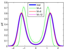
Figure 2: Approximated PDFs to the order $M$.

4.2 Online approximation of the Gibbs density of the parameter

In our analysis, we will assume the following model.

$$x_{t} =f_{\theta}(x_{t-1})+v_{t},\>v_{t}\sim N(0,\sigma^{2})$$

$$y_{t} =g(x_{t})+w_{t},\>w_{t}\sim N(0,\sigma_{o}^{2})$$

The posterior distribution for the static parameter is

$$p(\theta|x_{0:T})\propto p(\theta)\prod_{t=1}^{T}p(x_{t}|x_{t-1},\theta).$$

The product term, which requires linear time, is the bottleneck for this computation. A polynomial approximation to the transition function $f_{\theta}(\cdot)$ (the Taylor approximation around $\theta=0$) is:

$$f_{\theta}(x_{t-1}) =h(x_{t-1},\theta)=\sum_{i=0}^{M}\underbrace{\frac{1}{i!}\frac{d^{i}h(x_{t-1},\theta^{i})}{d\theta}\big{|}_{\theta=0}}_{H^{i}(x_{t-1})}\theta^{i}+R_{M}(\theta)$$

$$=\sum_{i=0}^{M}H^{i}(x_{t-1})\theta^{i}+R_{M}(\theta)=\hat{f}(\theta)+R_{M}(\theta)$$

where $R_{M}$ is the error for the $M$-dimensional Taylor approximation. We define coefficients $J^{i}_{x_{t-1}}$ to satisfy $\left(\sum_{i=0}^{M}H^{i}(x_{t-1})\theta^{i}\right)^{2}=J^{2M}_{x_{t-1}}\theta^{2M}+\dots+J^{0}_{x_{t-1}}\theta^{0}$.

Let $\hat{p}(\theta\mid x_{0:T})$ denote the approximation to $p(\theta\mid x_{0:T})$ obtained by using the polynomial approximation to $f_{\theta}$ introduced above.

Theorem 3.

$\hat{p}(\theta\mid x_{0:T})$ is in the exponential family with the log-polynomial density

$$\log p(\theta)+$$ (12)

$$\underbrace{\begin{pmatrix}\theta^{1}\\ \vdots\\ \theta^{M}\\ \theta^{M+1}\\ \vdots\\ \theta^{2M}\end{pmatrix}^{T}}_{T(\theta)^{T}}.\underbrace{\begin{pmatrix}\frac{1}{\sigma^{2}}\sum_{k=1}^{T}x_{k}H^{1}(x_{k-1})-\frac{1}{2\sigma^{2}}\sum_{k=1}^{T}J^{1}_{x_{k-1}}\\ \vdots\\ \frac{1}{\sigma^{2}}\sum_{k=1}^{T}x_{k}H^{M}(x_{k-1})-\frac{1}{2\sigma^{2}}\sum_{k=1}^{T}J^{M}_{x_{k-1}}\\ -\frac{1}{2\sigma^{2}}\sum_{k=1}^{T}J^{M+1}_{x_{k-1}}\\ \vdots\\ -\frac{1}{2\sigma^{2}}\sum_{k=1}^{T}J^{2M}_{x_{k-1}}\end{pmatrix}}_{\eta(x_{0},\dots,x_{t})}$$

The proof is given in the supplementary material.

This form has finite dimensional sufficient statistics. Standard sampling from $p(\theta\mid x_{0:t})$ requires $O(t)$ time, whereas with the polynomial approximation we can sample from this structured density of fixed dimension in constant time (given that sufficient statistics were tracked). We can furthermore prove that sampling from this exponential form approximation is asymptotically correct.

Theorem 4.

Let $p_{T}(\theta\mid x_{0:T})$ denote the Gibbs distribution and $\widehat{p}_{T}(\theta\mid x_{0:T})$ its order $M$ exponential family approximation. Assume that parameter $\theta$ has support $\mathcal{S}_{\theta}$ and finite variance. Then as $M\to\infty,T\to\infty$, the KL divergence between $p_{T}$ and $\widehat{p}_{T}$ goes to zero.

$$\lim_{M,T\to\infty}D_{KL}(p_{T}\mid\mid\hat{p}_{T})=0$$

The proof is given in the supplementary material (Erol et al., 2013). Note that the analysis above can be generalized to higher dimensional parameters. The one dimensional case is discussed for ease of exposition.

In the general case, an order $M$ Taylor expansion for a $p$ dimensional parameter vector $\theta$ will have $M^{p}$ terms. Then each update of the sufficient statistics will cost $O(M^{p})$ per particle, per time step, yielding the total complexity $O(NTM^{p})$. However, as noted before, we can often exploit the local structure of $f_{\theta}$ to speed up the update step. Notice that in either case, the update cost per time step is fixed (independent of $T$).

5 Experiments

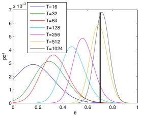
Figure 3: Sinusoidal dynamical model (SIN). Shrinkage of the Gibbs density $p(\theta\mid x_{0:T})$ with respect to time duration $T$. Note that as $T$ grows, the Gibbs density converges to the true parameter value.

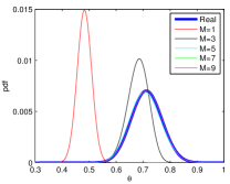
(a) Approximating Gibbs

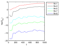
(b) KL-divergence

Figure 4: Sinusoidal dynamical model (SIN). 4(a) Convergence of the approximate densities to the Gibbs density $p(\theta\mid x_{0:1024})$ with respect to the approximation order $M$; 4(b) KL-divergence $D_{KL}(p\mid\hat{p})$ with respect to duration $T$ and approximation order $M$.

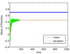
(a) Particle filter (SIR)

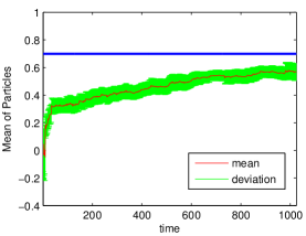
(b) Liu–West filter

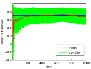
(c) EPF

Figure 5: Sinusoidal dynamical model (SIN). 5(a): Particle filter (SIR) with $N=50000$ particles. Note the failure to converge to the true value of parameter $\theta$ ($0.7$, shown as the blue line). 5(b): Liu–West filter with $N=50000$ particles. 5(c): EPF with $N=1000$ particles and $7$-th order approximation. Note both SIR and Liu–West do not converge, while the EPF converges quickly even with orders of magnitude fewer particles.

The algorithm is implemented for three specific cases. Note that the models discussed do not satisfy the Gaussian process model assumption of Storvik (2002).

5.1 Single parameter nonlinear model

Consider the following model with sinusoid transition dynamics (SIN):

$$x_{t} =\sin(\theta x_{t-1})+v_{t},\>v_{t}\sim N(0,\sigma^{2})$$

$$y_{t} =x_{t}+w_{t},\>w_{t}\sim N(0,\sigma_{\operatorname{obs}}^{2})$$ (13)

where $\sigma=1$, $\sigma_{\operatorname{obs}}=0.1$ and the Gaussian prior for parameter $\theta$ is $N(0,0.2^{2})$. The observation sequence is generated by sampling from SIN with true parameter value $\theta=0.7$.

Figure 3 shows how the Gibbs density $p(\theta\mid x_{0:t})$ shrinks with respect to time, hence verifying identifiability for this model. Notice that as $T$ grows, the densities concentrate around the true parameter value.

A Taylor approximation around $\theta=0$ has been applied to the transition function $\sin(\theta x_{t})$. Figure 4(a) shows the approximate densities for different polynomial orders for $T=1024$. Notice that as the polynomial order increases, the approximate densities converge to the true density $p(\theta\mid x_{0:1024})$.

The KL-divergence $D_{KL}(p\mid\mid\hat{p})$ for different polynomial orders (N) and different data lengths (T) is illustrated in Figure 4(b). The results are consistent with the theory developed in Section 2.

The degeneracy of a bootstrap filter with $N=50000$ particles can be seen from figure 5(a). The Liu–West approach with $N=50000$ particles is shown in 5(b). The perturbation is $\theta_{t}=\rho\theta_{t-1}+(1-\rho)\bar{\theta}_{t-1}+\sqrt{1-\rho^{2}}\operatorname{std}(\theta_{t-1})N(0,1)$, where $\rho=0.9$. Notice that even with $N=50000$ particles and large perturbations, the Liu–West approach converges slowly compared to our method. Furthermore, for high-dimensional spaces, tuning the perturbation parameter $\rho$ for Liu–West becomes difficult.

The EPF has been implemented on this model with $N=1000$ particles with a $7$-th order Taylor approximation to the posterior. The time complexity is $O(NT)$. The mean and the standard deviation of the particles are shown in figure 5(c).

5.2 Cauchy dynamical system

We consider the following model.

$$x_{t} =ax_{t-1}+\operatorname{Cauchy}(0,\gamma)$$ (14)

$$y_{t} =x_{t}+N(0,\sigma_{\operatorname{obs}})$$ (15)

Here $\operatorname{Cauchy}$ is the Cauchy distribution centered at $0$ and with shape parameter $\gamma=1$. We use $a=0.7$, $\sigma_{\operatorname{obs}}=10$, where the prior for the AR(1) parameter is $N(0,0.2^{2})$. This model represents autoregressive time evolution with heavy-tailed noise. Such heavy-tailed noises are observed in network traffic data and click-stream data. The standard Cauchy distribution we use is

$$f_{v}(v;0,1)=\frac{1}{\pi(1+v^{2})}=\exp\left(-\log(\pi)-\log(1+v^{2})\right).$$

We approximate $\log(1+v^{2})$ by $v^{2}-v^{4}/2+v^{6}/3-v^{8}/4+\dots$ (the Taylor approximation at 0).

Figure 6(a) shows the simulated hidden state and the observations ($\sigma_{obs}=10$). Notice that the simulated process differs substantially from a standard AR(1) process due to the heavy-tailed noise. Storvik’s filter cannot handle this model since the necessary sufficient statistics do not exist.

Figure 6(b) displays the mean value estimated by a bootstrap filter with $N=50000$ particles. As before the bootstrap filter is unable to perform meaningful inference. Figure 6(c) shows the performance of the Liu–West filter with both $N=100$ and $N=10000$ particles. The Liu–West filter does not converge for $N=100$ particles and converges slowly for $N=10000$ particles. Figure 6(d) demonstrates the rapid convergence of the EPF for only $N=100$ particles with 10th order approximation. The time complexity is $O(NT)$.

Our empirical results confirm that the EPF proves useful for models with heavy-tailed stochastic perturbations.

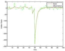
(a) Data sequence

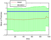
(b) Particle filter (SIR)

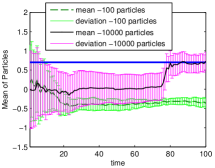
(c) Liu–West filter

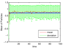
(d) EPF

Figure 6: Cauchy dynamical system. 6(a): Example sequences for hidden states and observations. 6(b): Particle filter estimate with 50000 particles. 6(c): Liu–West filter with 100 and 10000 particles. 6(d): EPF using only 100 particles and 10th order approximation. Note EPF converges to the actual value of parameter $a$ (=0.7, in blue line) while SIR does not even with orders of magnitude more particles, neither does Liu–West with the same number of particles.

5.3 Smooth Transition AR model

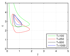
(a) Gibbs density

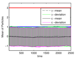
(b) Liu–West filter

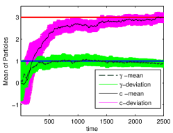
(c) EPF

Figure 7: STAR model. 7(a): Shrinkage of the Gibbs density $p(\gamma,c\mid x_{0:t})$ with respect to time. 7(b): Liu–West filter using 50000 particles. 7(c): EPF using 100 particles and 9th order approximation. Note the EPF’s estimates for both parameters converge to the actual values quickly even with only 100 particles, while Liu–West does not converge at all.

The smooth transition AR (STAR) model is a smooth generalization of the self-exciting threshold autoregressive (SETAR) model, (van Dijk et al., 2002). It is generally expressed in the following form.

$$x_{t}= \left(a_{1}x_{t-1}+a_{2}x_{t-2}+\dots+a_{p}x_{t-p}\right)\left[1-G(x_{t-d};\gamma,c)\right]$$

$$+ \left(b_{1}x_{t-1}+b_{2}x_{t-2}+\dots+b_{p}x_{t-p}\right)\left[G(x_{t-d};\gamma,c)\right]+\epsilon_{t}$$

where $\epsilon_{t}$ is i.i.d. Gaussian with mean zero and variance $\sigma^{2}$ and $G(\cdot)$ is a nonlinear function of $x_{t-d}$, where $d>0$. We will use the logistic function

$$G(y_{t-d};\gamma,c)=\frac{1}{1+\exp\left(-\gamma(x_{t-d}-c)\right)}$$ (16)

For high $\gamma$ values, the logistic function converges to the indicator function, $\mathbb{I}(x_{t-d}>c)$, forcing STAR to converge to SETAR (SETAR corresponds to a switching linear–Gaussian system). We will use $p=1=d$, where $a_{1}=0.9$ and $b_{1}=0.1$ and $\sigma=1$ (corresponding to two different AR(1) processes with high and low memory). We attempt to estimate parameters $\gamma,c$ of the logistic function, which have true values $\gamma=1$ and $c=3$. Data (of length $T=1000$) is generated from the model under fixed parameter values and with observation model $y_{t}=x_{t}+w_{t}$, where $w_{t}$ is additive Gaussian noise with mean zero and standard deviation $\sigma_{\operatorname{obs}}=0.1$. Figure 7(a) shows the shrinkage of the Gibbs density $p(\gamma,c\mid x_{0:T})$, verifying identifiability.

The non-separable logistic term is approximated as

$$\frac{1}{1+\exp\left(-\gamma(x_{t-1}-c)\right)}$$

$$\approx\frac{1}{2}-\frac{1}{4}\gamma(c-x_{t-1})+\frac{1}{48}\gamma^{3}(c-x_{t-1})^{3}+\dots$$

Figure 7(b) displays the failure of the Liu–West filter for $N=50000$ particles. Figure 7(c) shows the mean values for $\gamma,c$ from EPF for only $N=100$ particles with $9$th order Taylor approximation. Sampling from the log-polynomial approximate density is done through the random-walk Metropolis–Hastings algorithm. For each particle path, at each time step $t$, the Metropolis–Hastings sampler is initialized from the parameter values at $t-1$. The burn-in period is set to be 0, so only one MH step is taken per time step (i.e., if a proposed sample is more likely it is accepted, else it is rejected with a specific probability). The whole filter has time complexity $O(NT)$.

6 Conclusion

Learning the parameters of temporal probability models remains a significant open problem for practical applications. We have proposed the extended parameter filter (EPF), a novel approximate inference algorithm that combines Gibbs sampling of parameters with computation of approximate sufficient statistics. The update time for EPF is independent of the length of the observation sequence. Moreover, the algorithm has provable error bounds and handles a wide variety of models. Our experiments confirm these properties and illustrate difficult cases on which EPF works well.

One limitation of our algorithm is the complexity of Taylor approximation for high-dimensional parameter vectors. We noted that, in some cases, the process can be decomposed into lower-dimensional subproblems. Automating this step would be beneficial.

Appendix A Storvik’s filter as a Kalman filter

Let us consider the following model.

$${x}_{t} ={\mathbf{A}}{x}_{t-1}+{v}_{t},\>{v}_{t}\sim N(0,{\mathbf{Q}})$$

$${y}_{t} ={\mathbf{H}}{x}_{t}+{w}_{t},\>{w}_{t}\sim N(0,{\mathbf{R}})$$ (17)

We will call the MMSE estimate Kalman filter returns as ${x}_{t\mid t}=\mathbb{E}[{x}_{t}\mid{y}_{0:t}]$ and the variance ${\mathbf{P}}_{t\mid t}=cov({x}_{t}\mid{y}_{0:t})$. Then the update for the conditional mean estimate is as follows.

$${x}_{t\mid t}={\mathbf{A}}{x}_{t-1\mid t-1}$$

$$+\underbrace{{\mathbf{P}}_{t\mid t-1}{\mathbf{H}}^{T}({\mathbf{H}}{\mathbf{P}}_{t\mid t-1}{\mathbf{H}}^{T}+{\mathbf{R}})^{-1}}_{{\mathbf{K}}_{t}}({y}_{t}-{\mathbf{H}}{\mathbf{A}}{x}_{t-1\mid t-1})$$

where as for the estimation covariance

$${\mathbf{P}}_{t\mid t-1} ={\mathbf{A}}{\mathbf{P}}_{t-1\mid t-1}{\mathbf{A}}^{T}+{\mathbf{Q}}$$

$${\mathbf{P}}_{t\mid t} =({\mathbf{I}}-{\mathbf{K}}_{t}{\mathbf{H}}){\mathbf{P}}_{t\mid t-1}$$ (18)

Matching the terms above to the updates in equation 2.3, one will obtain a linear model for which the transition matrix is ${\mathbf{A}}={\mathbf{I}}$, the observation matrix is ${\mathbf{H}}={\mathbf{F}}_{t}$, the state noise covariance matrix is ${\mathbf{Q}}={\mathbf{0}}$, and the observation noise covariance matrix is ${\mathbf{R}}={\mathbf{Q}}$

Appendix B Proof of theorem 1

Let us assume that ${x}\in\mathbb{R}^{d}$,$\theta\in\mathbb{R}^{p}$ and $f_{\theta}(\cdot):\mathbb{R}^{d}\rightarrow\mathbb{R}^{d}$ is a vector valued function parameterized by $\theta$. Moreover, due to the assumption of separability $f_{\theta}({x}_{t-1})=l({x}_{t-1})^{T}h(\theta)$, where we assume that $l(\cdot):\mathbb{R}^{d}\rightarrow\mathbb{R}^{m\times d}$ and $h(\cdot):\mathbb{R}^{p}\rightarrow\mathbb{R}^{m}$ and $m$ is an arbitrary constant. The stochastic perturbance will have the log-polynomial density $p({v}_{t})\propto\exp({\mathbf{\Lambda}}_{1}{v}_{t}+{v}_{t}^{T}{\mathbf{\Lambda}}_{2}{v}_{t}+\dots)$ Let us analyze the case of $p({v}_{t})\propto\exp({\mathbf{\Lambda}}_{1}{v}_{t}+{v}_{t}^{T}{\mathbf{\Lambda}}_{2}{v}_{t})$, for mathematical simplicity.

Proof.

$$\log p(\theta\mid{x}_{0:T})\propto\log p(\theta)+\sum_{t=1}^{T}\log p({x}_{t}\mid{x}_{t-1},\theta)$$

$$\propto\log p(\theta)+\sum_{t=1}^{T}{\mathbf{\Lambda}}_{1}\left({x}_{t}-l({x}_{t-1})^{T}h(\theta)\right)+$$

$$\>\>\>\left({x}_{t}-l({x}_{t-1})^{T}h(\theta)\right)^{T}{\mathbf{\Lambda}}_{2}\left({x}_{t}-l({x}_{t-1})^{T}h(\theta)\right)$$

$$\propto\log p(\theta)+\underbrace{\left(\sum_{t=1}^{T}-({\mathbf{\Lambda}}_{1}+2{x}_{t}^{T}{\mathbf{\Lambda}}_{2})l({x}_{t-1})^{T}\right)}_{{\mathbf{S}}_{1}}h(\theta)$$

$$+h^{T}(\theta)\underbrace{\left(\sum_{t=1}^{T}l(x_{t-1}){\mathbf{\Lambda}}_{2}l^{T}(x_{t-1})\right)}_{{\mathbf{S}}_{2}}h(\theta)+\mathrm{constants}$$

Therefore, sufficient statistics (${\mathbf{S}}_{1}\in\mathbb{R}^{1\times m}$ and ${\mathbf{S}}_{2}\in\mathbb{R}^{m\times m}$) exist. The analysis can be generalized for higher-order terms in ${v}_{t}$ in similar fashion. ∎

Appendix C Proof of theorem 2

Proposition 1.

Let $S(x)$ be a $M+1$ times differentiable function and $P(x)$ its order $M$ Taylor approximation. Let $I=(x-a,x+a)$ be an open interval around $x$. Let $R(x)$ be the remainder function, so that $S(x)=P(x)+R(x)$. Suppose there exists constant $U$ such that

$$\forall y\in I,\quad\left|f^{(k+1)}(y)\right|\leq U$$

We may then bound

$$\forall y\in I,\quad\left|R(y)\right|\leq U\frac{a^{M+1}}{(M+1)!}$$

We define the following terms

$$\epsilon =U\frac{a^{M+1}}{(M+1)!}$$

$$Z =\int_{I}\exp(S(x))dx$$

$$\hat{Z} =\int_{I}\exp(P(x))dx$$

Since $\exp(\cdot)$ is monotone and increasing and $\left|S(x)-P(x)\right|\leq\epsilon$, we can derive tight bounds relating $Z$ and $\widehat{Z}$.

$$Z =\int_{I}\exp(S(x))dx\leq\int_{I}\exp(P(x)+\epsilon)dx$$

$$=\hat{Z}\exp(\epsilon)$$

$$Z =\int_{I}\exp(S(x))dx\geq\int_{I}\exp(P(x)-\epsilon)dx$$

$$=\hat{Z}\exp(-\epsilon)$$

Proof.

$$D_{KL}(p||\hat{p})=\int_{I}\ln\left(\frac{p(x)}{\hat{p}(x)}\right)p(x)dx$$

$$=\int_{I}\left(S(x)-P(x)+\ln(\hat{Z})-\ln(Z)\right)p(x)dx$$

$$\leq\int_{I}\left|S(x)-P(x)\right|p(x)dx$$

$$+\int_{I}\left|\ln(\hat{Z})-\ln(Z)\right|p(x)dx$$

$$\leq 2\epsilon\propto\frac{a^{M+1}}{(M+1)!}\approx\frac{1}{\sqrt{2\pi(M+1)!}}\left(\frac{ae}{M+1}\right)^{M+1}$$

where the last approximation follows from Stirling’s approximation. Therefore, $D_{KL}(p||\hat{p})\rightarrow 0$ as $M\rightarrow\infty$. ∎

Appendix D Proof of theorem 3

Proof.

$$\log\hat{p}(\theta\mid x_{0:T}) =\log\left(p(\theta)\prod_{k=0}^{T}\hat{p}(x_{k}|x_{k-1},\theta)\right)$$

$$=\log p(\theta)+\sum_{k=0}^{T}\log\hat{p}(x_{k}\mid x_{k-1},\theta)$$

We can calculate the form of $\log\hat{p}(x_{k}\mid x_{k-1},\theta)$ explicitly.

$$\log\hat{p}(x_{k}\mid x_{k-1},\theta)=\log\mathcal{N}(\hat{f}(x_{k-1},\theta),\sigma^{2})$$

$$=-\log(\sigma\sqrt{2\pi})-\frac{(x_{k}-\hat{f}(x_{k-1},\theta))^{2}}{2\sigma^{2}}$$

$$=-\log(\sigma\sqrt{2\pi})-\frac{x_{k}^{2}-2x_{k}\hat{f}(x_{k-1},\theta)+\hat{f}(x_{k-1},\theta)^{2}}{2\sigma^{2}}$$

$$=-\log(\sigma\sqrt{2\pi})-\frac{x_{k}^{2}}{2\sigma^{2}}-\frac{\sum_{i=0}^{M}x_{k}H^{i}(x_{k-1})\theta^{i}}{\sigma^{2}}$$

$$\qquad+\frac{\sum_{i=0}^{2M}J^{i}_{x_{k-1}}\theta^{i}}{2\sigma^{2}}$$

Using this expansion, we calculate

$$\log\hat{p}(\theta\mid x_{0:T}) =\log p(\theta)+\sum_{k=0}^{T}\log\hat{p}(x_{k}\mid x_{k-1},\theta)$$

$$=\log p(\theta)-(T+1)\log(\sigma\sqrt{2\pi})$$

$$\qquad-\frac{1}{2\sigma^{2}}\left(\sum_{k=0}^{T}x_{k}^{2}\right)-T(\theta)^{T}\eta(x_{0},\dotsc,x_{T})$$

where we expand $T(\theta)^{T}\eta(x_{0},\dotsc,x_{T})$ as in 3. The form for $\log\hat{p}(\theta\mid x_{0:T})$ is in the exponential family. ∎

Appendix E Proof of theorem 4

Proof.

Assume that function $f$ has bounded derivatives and bounded support $I$. Then the maximum error satisfies $\left|f_{\theta}(x_{k-1})-\hat{f}_{\theta}(x_{k-1})\right|\leq\epsilon_{k}$. It follows that $\hat{f}_{\theta}(x_{k-1})^{2}-f_{\theta}(x_{k-1})^{2}=-\epsilon_{k}^{2}-2\hat{f}_{\theta}(x_{k-1})\epsilon_{k}\approx-2\hat{f}_{\theta}(x_{k-1})\epsilon_{k}$.

Then the KL-divergence between the real posterior and the approximated posterior satisfies the following formula.

$$D_{KL}(p_{T}||\hat{p}_{T})$$ (19)

$$\quad=\int_{\mathcal{S}_{\theta}}\left(\frac{1}{\sigma^{2}}\sum_{k=1}^{T}\epsilon_{k}(x_{k}-\hat{f}_{\theta}(x_{k-1}))\right)p_{T}(\theta|x_{0:T})d\theta$$

Moreover, recall that as $T\rightarrow\infty$ the posterior shrinks to $\delta(\theta-\theta^{*})$ by the assumption of identifiability. Then we can rewrite the KL-divergence as (assuming Taylor approximation centered around $\theta_{c}$)

$$\lim_{T\rightarrow\infty}D_{KL}(p_{T}||\hat{p}_{T})$$ (20)

$$=\frac{1}{\sigma^{2}}\lim_{T\to\infty}\sum_{k=1}^{T}\epsilon_{k}\int_{\mathcal{S}_{\theta}}(x_{k}-\hat{f}_{\theta}(x_{k-1}))p_{T}(\theta|x_{0:T})d\theta$$

$$=\frac{1}{\sigma^{2}}\lim_{T\to\infty}\sum_{k=1}^{T}\epsilon_{k}\cdot$$ (21)

$$\qquad\left(x_{k}-\sum_{i=0}^{M}H^{i}(x_{k-1})\int_{\mathcal{S}_{\theta}}(\theta-\theta_{c})^{i}p(\theta|x_{0:T})d\theta\right)$$

$$=\frac{1}{\sigma^{2}}\lim_{T\to\infty}\sum_{k=1}^{T}\epsilon_{k}\left(x_{k}-\sum_{i=0}^{M}H^{i}(x_{k-1})(\theta^{*}-\theta_{c})^{i}\right)$$

If the center of the Taylor approximation $\theta_{c}$ is the true parameter value $\theta^{*}$, we can show that

$$\lim_{T\rightarrow\infty}D_{KL}(p_{T}||\hat{p}_{T}) =\frac{1}{\sigma^{2}}\lim_{T\to\infty}\sum_{k=1}^{T}\epsilon_{k}\left(x_{k}-f_{\theta^{*}}(x_{k-1}))\right)$$

$$=\frac{1}{\sigma^{2}}\lim_{T\to\infty}\sum_{k=1}^{T}\epsilon_{k}v_{k}=0$$ (22)

where the final statement follows from law of large numbers. Thus, as $T\rightarrow\infty$, the Taylor approximation of any order will converge to the true posterior given that $\theta_{c}=\theta^{*}$. For an arbitrary center value $\theta_{c}$,

$$D_{KL}(p_{T}||\hat{p}_{T}) =\frac{1}{\sigma^{2}}\sum_{k=1}^{T}\epsilon_{k}\left(x_{k}-\sum_{i=0}^{M}H^{i}(x_{k-1})(\theta^{*}-\theta_{c})^{i}\right)$$ (23)

Notice that $\epsilon_{k}\propto\frac{1}{(M+1)!}$ (by our assumptions that $f$ has bounded derivative and is supported on interval $I$) and $H^{i}(\cdot)\propto\frac{1}{M!}$. The inner summation will be bounded since $M!>a^{M},\forall a\in\mathbb{R}$ as $M\rightarrow\infty$. Therefore, as $M\rightarrow\infty$, $D_{KL}(p||\hat{p})\rightarrow 0$. ∎

References

- Andrieu et al. [2005] C. Andrieu, A. Doucet, and V. Tadic. On-line parameter estimation in general state-space models. In Proceedings of the 44th Conference on Decision and Control, pages 332–337, 2005.
- Andrieu et al. [2010] Christophe Andrieu, Arnaud Doucet, and Roman Holenstein. Particle Markov chain Monte Carlo methods. Journal of the Royal Statistical Society: Series B (Statistical Methodology), 72(3):269–342, 2010.
- Arulampalam et al. [2002] Sanjeev Arulampalam, Simon Maskell, Neil Gordon, and Tim Clapp. A tutorial on particle filters for on-line non-linear/non-Gaussian Bayesian tracking. IEEE Transactions on Signal Processing, 50(2):174–188, 2002.
- Carvalho et al. [2010] Carlos M. Carvalho, Michael S. Johannes, Hedibert F. Lopes, and Nicholas G. Polson. Particle Learning and Smoothing. Statistical Science, 25:88–106, 2010. doi: 10.1214/10-STS325.
- Doucet and Johansen [2011] Arnaud Doucet and Adam M. Johansen. A tutorial on particle filtering and smoothing: fifteen years later. The Oxford Handbook of Nonlinear Filtering, pages 4–6, December 2011.
- Erol et al. [2013] Yusuf Erol, Lei Li, Bharath Ramsundar, and Stuart J. Russell. The extended parameter filter. Technical Report UCB/EECS-2013-48, EECS Department, University of California, Berkeley, May 2013. URL http://www.eecs.berkeley.edu/Pubs/TechRpts/2013/EECS-2013-48.html.
- Gilks and Berzuini [2001] Walter R. Gilks and Carlo Berzuini. Following a moving target – Monte Carlo inference for dynamic bayesian models. Journal of the Royal Statistical Society. Series B (Statistical Methodology), 63(1):127–146, 2001.
- Kalman [1960] Rudolf E. Kalman. A new approach to linear filtering and prediction problems. Transactions of the ASME – Journal of Basic Engineering, 82 (Series D):35–45, 1960.
- Kantas et al. [2009] Nicholas Kantas, Arnaud Doucet, Sumeetpal Sindhu Singh, and Jan Maciejowski. An overview of sequential Monte Carlo methods for parameter estimation in general state-space models. In 15th IFAC Symposium on System Identification, volume 15, pages 774–785, 2009.
- Liu and West [2001] Jane Liu and Mike West. Combined parameter and state estimation in simulation-based filtering. In Sequential Monte Carlo Methods in Practice. 2001.
- Neal [2003] Radford M. Neal. Slice sampling. Annals of Statistics, 31(3):705–767, 2003.
- Polson et al. [2008] Nicholas G. Polson, Jonathan R. Stroud, and Peter Müller. Practical filtering with sequential parameter learning. Journal of the Royal Statistical Society: Series B (Statistical Methodology), 70(2):413–428, 2008.
- Robert and Casella [2005] Christian P. Robert and George Casella. Monte Carlo Statistical Methods. Springer-Verlag New York, Inc., Secaucus, NJ, USA, 2005.
- Storvik [2002] Geir Storvik. Particle filters for state-space models with the presence of unknown static paramaters. IEEE Transactions on Signal Processing, 50(2):281–289, 2002.
- van Dijk et al. [2002] Dick van Dijk, Timo Ter svirta, and Philip Hans Franses. Smooth transition autoregressive models – a survey of recent developments. Econometric Reviews, 21:1–47, 2002.
- Welch and Bishop [1995] Greg Welch and Gary Bishop. An introduction to the Kalman filter, 1995.